Annular embeddings of permutations for arbitrary genus
Abstract
In the symmetric group on a set of size , let denote the conjugacy class of involutions with no fixed points (equivalently, we refer to these as “pairings”, since each disjoint cycle has length ). Harer and Zagier explicitly determined the distribution of the number of disjoint cycles in the product of a fixed cycle of length and the elements of . Their famous result has been reproved many times, primarily because it can be interpreted as the genus distribution for -cell embeddings in an orientable surface, of a graph with a single vertex attached to loops. In this paper we give a new formula for the cycle distribution when a fixed permutation with two cycles (say the lengths are , where ) is multiplied by the elements of . It can be interpreted as the genus distribution for -cell embeddings in an orientable surface, of a graph with two vertices, of degrees and . In terms of these graphs, the formula involves a parameter that allows us to specify, separately, the number of edges between the two vertices and the number of loops at each of the vertices. The proof is combinatorial, and uses a new algorithm that we introduce to create all rooted forests containing a given rooted forest.
1 Introduction
Let , and be the set of permutations of , for . When is even, let be the set of pairings on , which are partitions of the set into disjoint pairs (subsets of size ). We refer to the single element of as the empty pairing. Where the context is appropriate, we shall also regard as the conjugacy class of involutions with no fixed points in . In this latter context, each pair becomes a disjoint cycle consisting of that pair of elements. Of course, the number of pairings in is , with the empty product convention that .
Now, for and even, let , in disjoint cycle notation, and let . Let be the number of permutations in with cycles in the disjoint cycle representation, for . The generating series for these numbers are given by . Harer and Zagier [4] obtained the following result.
Theorem 1.1.
(Harer and Zagier [4]) For a positive, even integer , with ,
Other proofs of Theorem 1.1 have been given by Itzykson and Zuber [5], Jackson [6], Kerov [7], Kontsevich [8], Lass [10], Penner [12] and Zagier [15] (see also the survey by Zvonkin [16], Section 3.2.7 of Lando and Zvonkin [9] and the discussion in Section 4 of the paper by Haagerup and Thorbjornsen [2]). Recently, Goulden and Nica [3] gave a direct bijective proof of Theorem 1.1. In the present paper, we consider a similar bijective approach to extend this important result of Harer and Zagier to the case in which the permutation is replaced by a fixed permutation with two cycles in its disjoint cycle representation. Some additional notation is required.
Let , and let be the set of permutations of , for . Let be the set of pairings on , for , where is even (we refer to the single element of as the empty pairing). A pair in a pairing is called mixed if it consists of one element from and one element from . Where the context is appropriate, we shall also regard as the conjugacy class of involutions with no fixed points in . For , we consider the permutation , and let , and be the number of permutations in with cycles in the disjoint cycle representation, for . Consider the generating series
The main result of this paper is the following expression for .
Theorem 1.2.
For , with of the same odd-even parity and , we have
where
Note that Theorem 1.2 gives a summation of nonnegative terms, since for all choices of summation indices with (so that is nonzero), the difference is nonnegative. The proof of Theorem 1.2 is based on a combinatorial model that is developed in Section 2. As a consequence, it is sufficient to enumerate a particular graphical object that we call a paired array. We then give two combinatorial reductions, in Sections 3 and 5, in terms of a simpler class of paired arrays called vertical paired arrays. These are explicitly enumerated in Section 6, which allows us to complete the proof of Theorem 1.2. One of the combinatorial conditions on paired arrays is that two graphs associated with them must be acyclic. Because of this, a key component of Sections 5 and 6 is the enumeration of rooted forests which contain a given forest as a subgraph. Thus in Section 4 we give a new bijection for this fundamental combinatorial problem. However, before we turn to our combinatorial model and subsequent reductions, we consider some consequences of Theorem 1.2, and give some comparisons to results in the existing literature.
A major reason that Harer and Zagier’s result (Theorem 1.1) is important (as evidenced by so many published proofs) is that it can be restated as an equivalent geometric problem in terms of maps. A map is an embedding of a connected graph (with loops and multiple edges allowed) in an orientable surface, partitioning the surface into disjoint regions (called the faces of the map) that are homeomorphic to discs (this is called a two-cell embedding). A rooted map is a map with a distinguished edge and incident vertex (so, the map is “rooted” at that end of the distinguished edge). The well-known embedding theorem allows us to consider this as equivalent to a pair of permutations and their product (see, e.g., Tutte [14], where the terminology “rotation system” is used to describe this triple of permutations). From this point of view, the th coefficient in the generating series evaluated in Theorem 1.1 is equal to the number of rooted maps with vertex, edges and faces (where , as in Theorem 1.1). Denoting the genus of the surface in which such a map is embedded by , then the Euler-Poincaré Theorem implies that , or that .
Similarly, Theorem 1.2 has a geometric interpretation. Let be the conjugacy class of in which there are two disjoint cycles, of lengths and . Then the coefficient in the generating series is equal to times the number of rooted maps with vertices (of degrees and ), edges (exactly of which join the two vertices together, plus that are loops at the vertex of degree , plus that are loops at the vertex of degree ), and faces (where , as in Theorem 1.2). In this case, if we denote the genus of the surface in which such a map is embedded by , then we obtain .
Of course, since genus is a nonnegative integer, we must have , and indeed the coefficient of in the summation for given in Theorem 1.2 is zero, since the summand corresponding to (which has as a factor) is itself equal to zero. For the planar case, which corresponds to , the only nonzero summand that contributes to the coefficient of in the summation of Theorem 1.2 corresponds to , and this gives immediately that
This checks with the straightforward computation that one can make to determine this value by elementary means – there are edges between the two vertices; between the ends of these edges at each vertex is an even number of vertices, joined by loops without crossings (and there is Catalan number of such arrangements for each such even interval).
This explains the term “genus” in the title; the term “annular” is adapted from its usage in Mingo and Nica [11]. It refers to an equivalent embedding for a map with two vertices, in an annulus. The ends of the edges incident with one of the vertices (say the one of degree ) are identified with points arranged around the disc on the exterior of the annulus, and the ends incident with the other vertex are identified with points arranged around the disc on the interior of the annulus. The points corresponding to the two ends of an edge are joined by an arc in the interior of the annulus.
We have been able to find one relevant enumerative result (Jackson [6]) in the literature about such maps, in which the total number of edges is specified, but not the exact number joining the two vertices together. To compare this result to our main result, we must sum over (since the underlying graph must be connected, then , the number of edges joining the two vertices together, must be positive), and thus define
Then Jackson [6] has considered the case , and obtained the following result, restated in terms of our notation (by applying the proportionality constant ).
Theorem 1.3.
(Jackson [6]) For ,
By slightly modifying Jackson’s [6] integration argument we are able to obtain the following expression for , with arbitrary of the same parity.
Theorem 1.4.
For , with even, and ,
We have checked computationally, with the help of Maple, that Theorems 1.3 and 1.4 agree with Theorem 1.2, summed over , for a wide range of values of . However, we have been unable to prove this for all , since we have not been able to show that the sum over of the result of Theorem 1.2 is equal to the result of Theorem 1.4. Note that the summation in Theorem 1.4 can be made symmetrical in (so the ordering is not required) by changing the summation variable to .
The method employed in Jackson [6] for Theorem 1.3, and in many of the papers listed above that give proofs of Theorem 1.1, is matrix integration. However, we do not see how to adapt the matrix integration methodology to prove our main result, Theorem 1.2, since it doesn’t seem possible to specify that there are exactly edges joining the two vertices together in the matrix method. The simplicity of our result seems to suggest that an extended theory of matrix integration to allow a specified number of edges between particular vertices might be possible, and worth investigating. The simplicity of the result also suggests that there should be a more direct combinatorial proof than the one presented in this paper.
2 The combinatorial model
2.1 Paired surjections
The combinatorial model for our proof of Theorem 1.2 is based on a paired surjection, which has the following definition.
Definition 2.1.
For , with of the same odd-even parity, let be the set of ordered pairs , where has mixed pairs, and is a surjection from onto , satisfying the condition
| (1) |
Such an ordered pair is called a paired surjection. Let .
In the following result, the generating series evaluated in Theorem 1.2 is expressed in terms of the numbers of paired surjections. Paired surjections are closely related to shift-symmetric partitions, that arose in Goulden and Nica [3]. Indeed, the proof of the following result is identical to the proof of Proposition 1.3 in Goulden and Nica [3], and is hence omitted.
Proposition 2.2.
For , with of the same odd-even parity, we have
We consider , and construct various objects associated with . First let and , for . Let , and , and let , , and , . Suppose that is contained in , and that is contained in . Define by when , and by when .
Now, if , then (interpreting as ) condition (1) means that , so we have . This implies that the functional digraph of (the directed graph on vertex-set with an arc directed from to for each ) is actually a tree, in which all arcs are directed towards vertex (which we consider as the root of this tree). We denote this rooted tree by . Similarly, the functional digraph of , on vertex-set , is also a tree, with all arcs directed towards vertex (which we consider as the root of this tree). We denote this rooted tree by .
One condition that the paired surjection satisfies is that the number of mixed pairs containing an element of is equal to the number of mixed pairs containing an element of for all . (For the reason that this necessary condition arises, see the discussion of “unique label recovery” in the next section.) We call this the balance condition for . The fact that is a surjection is equivalent to , for , and we call this the nonempty condition for . The fact, established above, that the graphs of and are trees is called the tree condition for .
2.2 A graphical model
Now we consider a graphical representation for the paired surjection , called its labelled paired array. This is an array of cells, arranged in columns, indexed from left to right, and two rows. In column of row , place an ordered list of vertices, labelled by the elements of from left to right; in column of row , place an ordered list of vertices, labelled by the elements of from left to right. For each pair of draw an edge between the vertices whose labels are given by the pair.
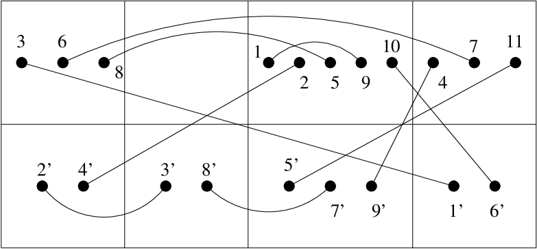

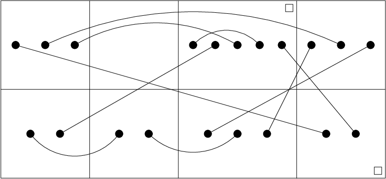
For example, when , consider , given by , and , , , . The corresponding labelled paired array is given in Figure 1, and the trees and are given in Figure 2.
Now suppose that we mark the cells in column of row and in column of row (by placing a small box in the top righthand corner of the marked cell in row 1, and in the bottom righthand corner of the marked cell in row 2), and remove the labels from all vertices – call the resulting object the paired array of . The ordered list of vertices in each cell is now to be interpreted as a generic totally ordered set, with the given left to right order, and the pairing now acts on these ordered sets in the obvious way. For example, the paired array determined from the labelled paired array displayed in Figure 1 is given in Figure 3.
What information have we lost when the labels are removed? The answer, perhaps surprisingly, is that no information is lost, since we have unique label recovery by applying condition (1) iteratively, as follows: for the first row, place label on the leftmost vertex in the marked cell of row ; for each from to , place label on the leftmost unlabelled vertex in column of row . The same process applied to the second row will place labels to on the vertices in row . (The reader can apply this to the paired array in Figure 3, to check that indeed the labelled paired array in Figure 1 is recovered in this way.) The proof that this process always works for a paired array satisfying the balance, nonempty and tree conditions (and the proof that these conditions are necessary for this process to work) requires only a slight modification of the results in Section 3 of [3], and is not given here (note that neither the functions and , nor the trees and , depend on the labels of the vertices, and the number of mixed pairs incident with the vertices in each cell of the paired array also does not depend on the labels, so the balance, nonempty and tree conditions can be checked on the paired array alone).
2.3 Paired arrays
This motivates us to define a paired array in the abstract (and not as obtained by removing the labels from a labelled paired array), and in fact to extend it to a more general class of objects, in the following definition.
Definition 2.3.
For , with of the same odd-even parity, we define to be the set of arrays of cells, arranged in columns and rows, subject to the following conditions:
- •
Each cell contains an ordered list of vertices, so that there is a total of vertices in the first row, and vertices in the second row. The vertices are paired (in the language of graph theory, there is a perfect matching on the vertices), so that pairs join a vertex in the first row to a vertex in the second row (these are the mixed pairs). The number of mixed pairs containing a vertex in column of row is equal to the number of mixed pairs containing a vertex in column of row , for all (this is called the balance condition).
- •
There is at least one marked (with a small box) cell in row , and we denote the set of such columns by . There is at least one marked (with a small box) cell in row , and we denote the set of such columns by . There is at least one vertex in every column that is not contained in (this is called the nonempty condition).
- •
Denote the set of columns in which there is at least one vertex in row by , and the set of columns in which there is at least one vertex in row by . Define the function as follows: if the rightmost vertex in column of row is paired with a vertex in column , then . Similarly, define as follows: if the rightmost vertex in column of row is paired with a vertex in column , then . The functional digraph of is a forest with components (called the rightmost forest for row ); each component is a tree in which all edges are directed towards an element of (and this is called the root of that tree). The functional digraph of is a forest with components (called the rightmost forest for row ); each component is a tree in which all edges are directed towards an element of (and this is called the root of that tree). Together, these specify the forest condition.
The elements of are called paired arrays. A paired array is defined to be canonical if . Define to be the set of canonical paired arrays in , and .
The uniqueness of label recovery described in the previous section proves that there is a bijection (via labelled paired arrays) between the set of paired surjections and the set of canonical paired arrays, so we have
| (2) |
(It is straightforward to verify that the conditions for canonical paired arrays imply that every column is nonempty.) In this paper we shall determine , and hence the generating series via Proposition 2.2, by giving a combinatorial reduction for canonical paired arrays, thus directly determining .
3 Removing redundant pairs and minimal paired arrays
A redundant pair in a paired array is a vertex pair that is not mixed, and does not contain a vertex that is rightmost in an unmarked cell. A minimal paired array is a paired array without redundant pairs. We define to be the set of minimal, canonical paired arrays in , and . In our next result, we remove redundant pairs from a canonical paired array, and thus show that the enumeration of canonical paired arrays can be reduced to the enumeration of minimal, canonical paired arrays.
Theorem 3.1.
For , with of the same odd-even parity, we have
Proof.
For the proof, it is convenient to introduce some notation. A partial pairing on is a pairing on a set of even cardinality. If , then we also call it an -partial pairing. For each of these partial pairings , we call the support, and denote this by . Let be the set of -partial pairings on . Similarly, let be the set of -partial pairings on .
Consider an arbitrary . We now describe a construction for three objects, , and , obtained from . We begin by attaching the numbers to the vertices and the small box in row of , from left to right (under the interpretation that all vertices in column are to the left of all vertices in column for , and that the small box representing a marking is rightmost in its cell). Let be the partial pairing consisting of pairs of numbers attached to the redundant pairs in row of . We follow the analogous procedure for row : we attach primed numbers to the vertices and small box in row , and let be the partial pairing consisting of the pairs of (primed) numbers attached to the redundant pairs in row of . Third, we remove all redundant pairs (both vertices and edges) from , to get the paired array , with the same marked cells as . The vertices in each cell of have the same relative order as they did in . For example, if is the paired array in Figure 3, then we have , , and is given in Figure 4.
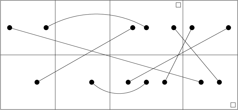
Now, the only vertex that can be numbered in row is the rightmost vertex of the rightmost nonempty cell in row (if this cell is not marked), but this vertex cannot appear in a redundant pair since it is rightmost in an unmarked cell. This implies that the numbers on redundant pairs in row all fall in the range , and so is a partial pairing on . Similarly, is a partial pairing on . Also, since the redundant pairs that were removed in the construction do not involve the rightmost vertex in any nonempty cell, has the same rightmost functions and as , and the same mixed pairs as , so it must satisfy the balance, nonempty and forest conditions, which implies that is a minimal paired array. Thus we have a mapping
We now prove that is a bijection. It is sufficient to describe the inverse mapping, so that we can uniquely recover from an arbitrary triple . Given , let , , and , . Number the vertices and small box in row of with the elements of . Then insert vertices numbered with the elements of , so that the numbers on all vertices and the small box in row increase from left to right, and so that the vertex numbered with is placed in the same cell as either the vertex or small box numbered with . Inserting vertices numbered from in row using an analogous process, pairing the inserted vertices with and , and removing the numbers, we arrive at a paired array . It is straightforward to check that satisfies the balance, nonempty, and tree conditions, and that the process described above reverses the numbering scheme used in the mapping . Thus, we have described the mapping , and our proof that is a bijection is complete. The result follows from the easily established facts that , . ∎
4 A bijection for rooted forests
In this section, we detour to consider the basic combinatorial question of how many rooted forests with a given set of root vertices contain a given rooted forest. We give a bijection for this that differs from the standard ones in the literature, like the Cycle Lemma (see, e.g., [13], p. 67) or the Prüfer Code (see, e.g., [13], p. 25), because it is more convenient for our constructions involving paired arrays.
Suppose we have a rooted forest (all edges directed towards a root vertex in each component) on vertex-set , whose components are the rooted trees , . Suppose the root vertex of is , , and the root vertex of is , . For convenience, we order the trees so that , , and we let denote the union of the sets of vertices in the trees .
Theorem 4.1 (Forest Completion Theorem).
There is a bijection between and the set of rooted forests on vertex-set with root vertices that contain as a subforest.
Proof.
We describe such a mapping, which we call the “Forest Completion Algorithm” (FCA). Consider the -tuple . We construct the forest corresponding to iteratively, in stages . At every stage, we have a forest containing as a subforest, a permutation of , and a sequence in . Initially, at stage , we have , is the identity permutation and . Then, for :
- •
if is in a different component of from , then add an arc directed from to in , and leave and unchanged;
- •
otherwise (so is in the same component of as ), add an arc directed from to in (to obtain the new ), switch and in , and switch and in .
The forest corresponding to the -tuple is the terminating forest . We call the terminating permutation the “Forest Completion Permutation” (FCP). The significance of the FCP is that it identifies precisely the arcs that are added to – they are , . In our examples throughout the paper, we shall specify the second line in the two line representation of – the list of images .
In Figure 5 we give an example of the FCA with , , . The trees , , , with , , , are given in the box at the top left; the trees , , with , , are given in the box at the top right. Then, corresponding to the triple , we construct the forest at the bottom of Figure 5. The corresponding FCP is .

In analyzing this mapping, it is convenient to use the term “safe” to describe a vertex in a component of a forest rooted at one of the vertices . Thus, initially, is safe. It is trivial to prove by induction that, after stage , for , is a forest with root vertices , and that is safe for (which implies that are in different components of from ). Thus, at stage , is indeed in a different component of from , so we successfully add the final arc from to , to obtain a terminating forest rooted at (this explains our use of “safe” – for extending our forest, it is always safe to add the new arc directed to ). This proves that the FCA does indeed produce a rooted forest on vertex-set with root vertices that contains as a subforest.
To prove that the FCA is a bijection, we describe its inverse. Suppose that we are given a rooted forest on vertex-set , with root vertices , and that we wish to remove the arcs directed from to , , where are distinct non-root vertices, with the convention that . We proceed iteratively, through stages . At every stage we have a subforest of , a permutation of , and a sequence in . Initially, at stage , we have , is the identity permutation, and . Then, for , remove the arc from to in (to get the new ), and:
- •
if is safe for (the new) , leave and unchanged;
- •
otherwise (so is not safe for ), switch and in , and switch and in .
We claim that the -tuple corresponding to the forest is the terminating -tuple , so that this mapping uniquely reverses the FCA. In fact, it is easy to establish that this mapping uniquely reverses the FCA stage by stage, since it is trivial to prove by induction that the values of and after stage of the above mapping are exactly the same as and after stage of the FCA. It is also easy to prove that the FCP is given by for the terminating .
The result follows, since the FCA is a bijection between the required sets. ∎
Of course, it is an immediate enumerative consequence of Theorem 4.1 that there are rooted forests on vertex-set with root vertices that contain as a subforest. In the special case (so that has no edges) this gives the classical result that there are rooted forests on vertex-set , with a prescribed set of root vertices (see, e.g., [13], p. 25).
5 Removing non-mixed pairs and vertical paired arrays
A vertical paired array is a paired array in which all pairs are mixed. We define to be the set of vertical paired arrays in , in which there are marked cells in row and marked cells in row , for , and let .
In our next result, we remove non-mixed pairs from a minimal, canonical paired array, and thus show that the enumeration of minimal, canonical paired arrays can be reduced to the enumeration of vertical paired arrays. We use the following notation. For a finite set , let denote the set of -tuples consisting of distinct elements of . Thus , where and is the falling factorial: for positive integers , ; for , ; otherwise .
Theorem 5.1.
For of the same odd-even parity, let and . Then
Proof.
Note that every element of has exactly and non-mixed pairs in the top and bottom rows, respectively. Taking an arbitrary , we now describe a mapping that is initially identical to that used in the proof of Theorem 3.1. We attach the numbers to the vertices and the small box in row , using the same left to right convention as in the proof of Theorem 3.1. Let the pairs of numbers attached to the non-mixed pairs in row be denoted by , where are attached to the rightmost vertices in these pairs (with ), and are attached to the other (not rightmost in their cell) vertices in these pairs.
Suppose that the marked cell in row is in column , and that the rightmost tree for row of is , so is rooted at vertex . Now run the inverse of the FCA on , to remove the arcs directed from to , , (here, denotes the column in which the number appears) and let be the corresponding FCP. Let .
We follow the analogous procedure for row : we attach primed numbers to the vertices and small box in row . Let the pairs of numbers attached to the non-mixed pairs in row be denoted by , where are attached to the rightmost vertices in these pairs (with ), and are attached to the other (not rightmost in their cell) vertices in these pairs.
Suppose that the marked cell in row is in column , and that the rightmost tree for row of is , so is rooted at vertex . Now run the inverse of the FCA on , to remove the arcs directed from to , , and let be the corresponding FCP. Let .
Finally, we mark the cells in row containing (in addition to the existing marked cell in column ), and the cells in row containing (in addition to the existing marked cell in column ), and then remove all non-mixed pairs (both vertices and edges) from , to get the vertical paired array . The vertices in each cell of have the same relative order as they did in .
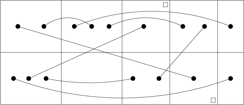

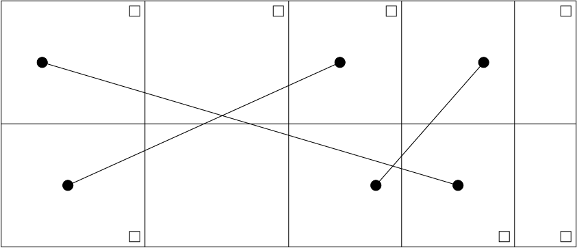
For example, suppose that is the paired array in Figure 6. Then we have , with , , , , , , and , with , , , . We have , , and the trees and are given in Figure 7. When we run the inverse of the FCA on to remove the arcs , and (for which we use dashed lines in Figure 7), we obtain as the FCP, which gives . When we run the inverse of the FCA on to remove the arcs and (for which we use dashed lines in Figure 7), we obtain as the FCP, which gives . The vertical paired array in this example is given in Figure 8.
Now, for the same reasons as in the proof of Theorem 3.1, we have for , so , and similarly, . Thus we have a mapping
In fact, is a bijection. Before proving this, for , we first note the key dependencies between and that follow from the FCA: let and denote the rightmost forests of for rows and , respectively. Then, in with numbers attached as in the construction above, the column containing the vertex whose number is the last entry of is contained in the component of rooted at . Similarly, the column containing the vertex whose number is the last entry of is contained in the component of rooted at . For example, for given in Figures 6–8, the last entries of and are and , respectively, corresponding to vertices of in columns and , respectively. Now, the forests and in this case are obtained from the trees and , respectively, by removing the dashed edges in Figure 7. Then, indeed, vertex is contained in the component of rooted at , and vertex is contained in the component of rooted at .
We now prove that is a bijection by describing the inverse mapping, so that we can uniquely recover from an arbitrary triple . Let denote the rightmost forest of for row . Let denote the set consisting of the entries in , and let , . Next (as a generalization of the procedure for the inverse of described in the proof of Theorem 3.1), we number the vertices and small boxes in row of with the elements of . Then insert vertices numbered with the elements of , so that the numbers on all vertices and small boxes increase from left to right (with any small box regarded as the rightmost object in its cell) and so that the the vertex numbered with is placed in the same cell as the object numbered with . Now suppose that , and use the key dependency noted above: let the column containing the vertex numbered be contained in the component of rooted at vertex . Let denote the numbers attached to the small boxes that are not in column (the columns containing are the root vertices for the components of not rooted at ). Now, apply the FCA on -tuple , to give the tree rooted at , that contains the forest as a subforest. Let be the FCP. Finally, replace the small boxes numbered by rightmost vertices (in the same cells) numbered , pair the vertex numbered with the vertex numbered , , and remove the numbers from row . Repeat the analogous process for row , and we arrive at a minimal paired array . It is straightforward to check that the process described above reverses . Thus, we have described , and our proof that is a bijection is complete. The result follows immediately. ∎
6 Enumeration of vertical paired arrays
For every column of a vertical paired array, the cells in rows and have the same number of vertices, because of the balance condition. A full, vertical paired array is a vertical paired array with a positive number of vertices in every column. Let be the set of full, vertical paired arrays in , and . In Theorem 6.1 we shall give an explicit construction for the elements of , and thus obtain an explicit formula for . To help in the proof of this result, we first introduce some terminology and notation associated with an arbitrary . A vertex is said to be dependent if it is paired with the rightmost vertex of an unmarked cell (in the other row). If the rightmost vertex of an unmarked cell in row , column is paired with the rightmost vertex of an unmarked cell in row , column , then we call this a shared pair of . In this case, the rightmost forest for row of contains arc and the rightmost forest for row of contains arc , and we call each of these a shared arc.
Now, canonically number the vertices in row of , from left to right, and number the vertices in row of , from left to right. Let be the subforest of with only the shared arcs of . Suppose that has non-shared arcs, corresponding to pairs , where , and are rightmost vertices in their (unmarked) cells. Run the inverse of the FCA on the forest , to obtain the subforest by removing the non-shared arcs directed from to , , and let be the corresponding FCP. Define . If all arcs of are shared, then let be the vertex in row that is paired with the rightmost non-dependent vertex in row (we call this the non-FCA option). In both cases, define , and let be the vertices on the unique directed path in from vertex to the root vertex () of the component of containing . Thus , and the cell in row , column is marked, and the cell in row , column is not marked, . Also, the cell in row , column is not marked, . Now define to be the subforest of containing the arcs , . Suppose that has arcs that are not in , corresponding to pairs , where , and are rightmost vertices in their (unmarked) cells. Run the inverse of the FCA on the forest , to obtain the subforest by removing the arcs directed from to , , and let be the corresponding FCP. Define . If , let be the vertex in row that is paired with the rightmost non-dependent vertex in row (again, we call this the non-FCA option). Let , which we call the tail of . The tail length is . We say that is in the tail when the column containing vertex is one of . The type of is given by . If the cells in rows and of column in have vertices, , then we say that has shape . Note that , and that is positive for all , so is a composition of with parts.

For example, suppose that is the full, vertical paired array given at the top of Figure 9, with , , , , shape , and rightmost forests and given at the bottom of Figure 9. The lines joining the pairs in are of various types (and the same type of line is used in the rightmost forests when the pair corresponds to an edge in one or other of these forests): a thick solid line indicates a shared pair in the tail, a thick dashed line a shared pair not in the tail, a thick dashed and dotted line a pair contributing to only, a thin solid line a pair contributing to only, and a thin dashed line a pair that contributes to neither of . When we run the inverse of the FCA to remove the arcs and from , we obtain the ordered pair , and hence obtain as indicated in Figure 9, contained in column . Thus the tail is , of length . When we run the inverse of the FCA to remove the arcs , , , and from , we obtain the -tuple , and hence obtain as indicated in Figure 9, contained in column . Thus we conclude that has type .
Theorem 6.1.
For , , we have
Proof.
Each paired array in has a unique type and shape, and we can uniquely construct those of given type and shape as follows. For the given shape, we begin with a by array, with each cell containing an ordered set of vertices of prescribed size. Then we pair these vertices (all are mixed pairs) in all possible ways for the given type in four stages. First, we pair the rightmost vertices as prescribed by the tail. Second, we use the FCA to pair the rightmost vertices in row (note that is safe, by construction). Third, we use the FCA to pair the unpaired rightmost vertices in row (note that is safe, by construction). Fourth, we pair the remaining vertices arbitrarily. (In addition, along the way, we have to choose the marked cells in a consistent fashion.) In this way, for each composition of with parts and , we enumerate elements of with shape and tail of length . There are three cases:
Case 1 (Vertex is not rightmost in its cell): There are choices for , which then fixes . There are then choices for , and then of the pairs are determined. This leaves choices for (any vertex not yet paired in row ). Now mark the cell in row , column . Also, if is in the tail, mark the cell in row , column , or if is not in the tail, mark the cell in row of the column that contains ( is in row ). Choose, from the cells not in the tail or already marked, cells to mark in the top row, and cells to mark in the bottom row. Now pair the unpaired rightmost vertices of unmarked cells in row with vertices in row to satisfy the forest condition, using vertex as the safe position. There are possible choices for this, from the FCA. Suppose that there are unmarked cells in row whose rightmost vertices are not yet paired. Then pair these with vertices in row to satisfy the forest condition, using vertex as the safe position. There are possible choices for this, from the FCA. Finally, there are ways to pair the remaining vertices, arbitrarily. But , and we conclude that the number of elements in with shape and tail of length in this case is
| (3) |
(It is straightforward the check that these cardinalities are correct when we use the non-FCA options also.)
Case 2 (Vertex is rightmost in its cell, and is in the tail): The number of choices for and is . Then , and of the pairs, are uniquely determined. The cell in row , column is marked. The cell in row , column is marked for two reasons – because is in the tail, and because the cell contains , rightmost, so that will be paired with a non-dependent vertex in row . The rest of the enumeration proceeds as in Case 1, and we conclude that the number of elements in with shape and tail of length in this case is
| (4) |
Case 3 (Vertex is rightmost in its cell, and is not in the tail): The number of choices for and is , and then together with of the pairs are uniquely determined. In this case three different cells must now be marked: in row , column ; in row , column ; in row of the column that contains . There are then ways to choose which other cells are marked, and the rest of the enumeration proceeds as in Cases 1 and 2. We conclude that the number of elements in with shape and tail of length in this case is
| (5) |
In the next result, we give an explicit enumeration for vertical paired arrays, by applying Theorem 6.1. The proof is quite technical, involving generating functions and a hypergeometric summation.
Theorem 6.2.
For , , we have
Proof.
If a column in a vertical paired array has no vertices, then at least one of the cells in rows and of that column must be marked, from the nonempty condition. Thus, suppose that a vertical paired array with mixed pairs and columns, has columns with no vertices and with a positive number of vertices (the same number in both rows of such columns). Of the columns with no vertices, suppose that are marked in row only, are marked in row only, and that are marked in both row and (we use this parameterization for convenience in determining the summations below). Then we have
| (6) |
where
But, from Theorem 6.1, we have
where we use the notation to denote the coefficient of in the expansion of . Now
which gives
| (7) |
where, summing over by the binomial theorem, we have
But, changing variables in (7), we have
so from (6) we obtain
where
Now, for this latter sum over , we observe that the ratio of the st term to the th term is a rational function of , which implies that it is a hypergeometric sum. In particular, using the standard notation for hypergeometric series, we have
where the second last equality follows from the Pfaff-Saalschütz Theorem for hypergeometric summations (see, e.g., Theorem 2.2.6 on page 69 of [1]). The result follows immediately. ∎
We finish with the proof of our main result, now that we have completed all the intermediate results in our reduction.
Acknowledgements
This work was supported by a Discovery Grant from NSERC (IG) and by a USRA Award from NSERC (WS). We are grateful to Andu Nica for helpful discussions and suggestions.
References
- 1.
G. E. Andrews, R. Askey and R. Roy, “Special functions”, Encyclopedia of Mathematics and its Applications, Vol. 71, Cambridge University Press, 1999.
- 2.
U. Haagerup and S. Thorbjornsen, Random matrices with complex Gaussian entries, Expositiones Math., 21 (2003), 293–337.
- 3.
I. P. Goulden and A. Nica, A direct bijection for the Harer-Zagier formula, J. Comb. Theory (A), 111 (2005), 224–238.
- 4.
J. Harer and D. Zagier, The Euler characteristic of the moduli space of curves, Inventiones Mathematicae, 85 (1986), 457–486.
- 5.
C. Itzykson and J.-B. Zuber, Matrix integration and combinatorics of modular groups, Comm. Math. Phys., 134 (1990), 197–207.
- 6.
D. M. Jackson, On an integral representation for the genus series for -cell embeddings, Trans. Amer. Math. Soc., 344 (1994), 755–772.
- 7.
S. Kerov, Rook placements on Ferrers boards, and matrix integrals (English translation), J. Math. Sci. (New York), 96 (1999), 3531–3536.
- 8.
M. Kontsevich, Intersection theory on the moduli space of curves and the matrix Airy function, Comm. Math. Phys., 147 (1992), 1–23.
- 9.
S. K. Lando and A. K. Zvonkin, “Graphs on surfaces and their applications”, Springer-Verlag, Berlin, Heidelberg, 2004.
- 10.
B. Lass, Démonstration combinatoire de la formule de Harer-Zagier, C. R. Acad. Sci. Paris, 333, Série I (2001), 155–160.
- 11.
J. A. Mingo and A. Nica, Annular noncrossing permutations and partitions, and second-order asymptotics for random matrices, International Math. Research Notices, no. 28 (2004), 1413 – 1460.
- 12.
R. C. Penner, Perturbative series and the moduli space of Riemann surfaces, J. Diff. Geometry, 27 (1988), 35–53.
- 13.
R. P. Stanley, “Enumerative Combinatorics”, Vol. 2, Cambridge University Press, 1999.
- 14.
W. T. Tutte, “Graph Theory”, Addison-Wesley, London, 1984.
- 15.
D. Zagier, On the distribution of the number of cycles of elements in symmetric groups, Nieuw Archief voor Wiskunde, 13 (1995), 489–495.
- 16.
A. Zvonkin, Matrix integrals and map enumeration: An accessible introduction, Combinatorics and Physics (Marseilles, 1995), Math. Comput. Modelling, 26 (1997), 281–304.