Event shape distributions in $e^{+}e^{-}$ annihilation processes are classical hadronic observables which can be measured very accurately and provide an ideal proving ground for testing our understanding of strong interactions. The deviation from simple two-jet configurations, which are a limiting case in event shapes, is proportional to the strong coupling constant, so that by comparing the measured event shape distribution with the theoretical predictions, one can determine the strong coupling constant $\alpha_{s}$. At LEP, a standard set of event shapes was studied in great detail [1, 4, 3, 2]: thrust $T$ [5] (which is substituted here by $\tau=1-T$), heavy jet mass $\rho$ [6], wide and total jet broadening $B_{W}$ and $B_{T}$ [7], $C$-parameter [8] and two-to-three-jet transition parameter in the Durham algorithm $Y_{3}$ [9]. The definitions of these variables, which we denote collectively as $y$ in the following, are summarised in [10]. The two-jet limit of each variable is $y\to 0$.

The theoretical prediction is made within perturbative QCD, expanded to a finite order in the coupling constant. This fixed order expansion is reliable only if the event shape variable is sufficiently far away from its two-jet limit. In the approach to this limit, event shapes display large infrared logarithms at all orders in perturbation theory, such that the expansion in the strong coupling constant fails to converge. Resummation of these logarithms yields a description appropriate to the two-jet limit. To explain event shape distributions over their full kinematical range, both descriptions need to be matched onto each other. Until very recently, the theoretical state-of-the-art description of event shape distributions was based on the matching of the next-to-leading-logarithmic approximation (NLLA, [11]) onto the fixed next-to-leading order (NLO, [12, 13, 14]) calculation. Using the newly available results of the next-to-next-to-leading order (NNLO) corrections for the standard set of event shapes [15, 16, 17, 18] introduced above, we derive here matching of the resummed NLLA onto the fixed order NNLO.

For two-particle final states, all above event shape variables have the fixed value $y=0$, consequently their distributions receive their first non-trivial contribution from three-particle final states, which, at order $\alpha_{s}$, correspond to three-parton final states. Therefore, both theoretically and experimentally, these distributions are closely related to three-jet production.

Fixed-order QCD corrections to event shape distributions were calculated long ago to next-to-leading order (NLO, [12, 13, 14]), and most recently to next-to-next-to-leading order (NNLO, [15, 16, 17]). At a centre-of-mass energy $Q$ and for renormalisation scale $\mu$, they take the form:

where

and where $\bar{A}$, $\bar{B}$ and $\bar{C}$ are the perturbatively calculated coefficients at LO, NLO, NNLO, normalised to $\sigma_{{\rm had}}$, explicit relations are given in [17] (note the different convention for the $\beta_{i}$ coefficients).

The resummation of large logarithmic corrections in the $y\to 0$ limit starts from the integrated cross section:

which has the following fixed-order expansion:

The fixed-order coefficients $\mathcal{A}$, $\mathcal{B}$, $\mathcal{C}$ can be obtained by integrating the distribution (1) and using $R(y_{{\rm max}},Q,\mu)=1$ to all orders, where $y_{{\rm max}}$ is the maximal kinematically allowed value for the shape variable $y$.

In the limit $y\to 0$ one observes that the perturbative $\alpha_{s}^{n}$–contribution to $R(y)$ diverges like $\alpha_{s}^{n}L^{2n}$, with $L=-\hbox{ln}\,y$ ($L=-\hbox{ln}\,(y/6)$ for $y=C$). This leading logarithmic (LL) behaviour is due to multiple soft gluon emission at higher orders, and the LL coefficients exponentiate, such that

where $g_{1}(\alpha_{s}L)$ is a power series in its argument.

For the event shapes considered here, leading and next-to-leading logarithmic (NLL) corrections can be resummed to all orders in the coupling constant, such that

where terms beyond NLL have been consistently omitted, and $\mu=Q$ ($x_{\mu}=1$) is used. In the case of the C-parameter further large logarithms around $C\,\approx\,0.75$, produce a so-called Sudakov shoulder in the distribution due to soft gluon divergences within the physical region [24].

By differentiating expression (5) with respect to $y$, one recovers the resummed differential event shape distributions, which yield an accurate description for $y\to 0$. The first complete calculation of next-to-next-to-leading logarithmic (NNLL) corrections to event shape distributions is available for the energy-energy correlation function [27], which is not part of the standard set of event shape observables. The application of soft-collinear effective field theory to event shape distributions [28] promises to yield results beyond NLL. Most recently, this formalism was applied to compute the resummed thrust distribution beyond NLL accuracy [29].

Closed analytic forms for the LL and NLL resummation functions $g_{1}(\alpha_{s}L)$, $g_{2}(\alpha_{s}L)$ are available for $\tau$ [19], $\rho$ [20], $B_{W}$ and $B_{T}$ [21, 22], $C$ [23] and $Y_{3}$ [25]. For the convenience of the reader, we collect them in uniform notation in an Appendix. They can be expanded as power series, such that:

To obtain a reliable description of the event shape distributions over a wide range in $y$, it is mandatory to combine fixed order and resummed predictions. To avoid the double counting of terms common to both, the two predictions have to be matched onto each other. A number of different matching procedures have been proposed in the literature, see for example [10] for a review. The by-now standard procedure is the so-called $\hbox{ln}\,R$-matching [11]. In this particular scheme, all matching coefficients can be extracted analytically from the resummed calculation, while most other schemes require the numerical extraction of some of the matching coefficients from the distributions at fixed order. Since the fixed order calculations face numerical instabilities in the region $y\to 0$, these matching coefficients can often be determined only within large errors. We shall therefore consider only the $\hbox{ln}\,R$-matching here. The $\hbox{ln}\,R$-matching at NLO is described in detail in [11], where the authors also anticipated the fixed-order NNLO corrections to be available shortly, and briefly outlined this matching scheme to NNLO.

In the $\hbox{ln}\,R$-matching scheme, the NLLA+NNLO expression is

The matching coefficients appearing in this expression can be obtained from (6) and are listed in Table 1. In the matching of $Y_{3}$, the constants ${\cal F}_{i}$ depend on the jet algorithm [25], in general, they can be determined only numerically. For the Durham-algorithm, one finds ${\cal F}_{2}=-\pi^{2}/32$ and ${\cal F}_{3}=0.0620\pm 0.0100$ [30], using the semi-numerical resummation method described in [26]. Numerical values of the matching coefficients for $N=3$, $N_{F}=5$ are given in Table 2.

To ensure the vanishing of the matched expression at the kinematical boundary $y_{\textrm{\tiny{max}}}$, the further substitution [10] is made:

where $y_{0}=6$ for $y=C$ and $y_{0}=1$ otherwise. $p=1$ and $x_{L}=1$ is taken as default.

The full renormalisation scale dependence of (7) is given by replacing the coupling constant, the fixed-order coefficients, the resummation functions and the matching coefficients as follows:

In the above, $g_{1}^{\prime}$ denotes the derivative of $g_{1}$ with respect to its argument. The LO coefficient ${\cal A}$ and the LL resummation function $g_{1}$, as well as the matching coefficients $G_{i\,i+1}$ remain independent on $\mu$.

The arbitrariness in the choice of the logarithm to be resummed can be quantified by varying the constant $x_{L}$. This variation implies also the modification of the NLL resummation function and of its coefficients

In Figures 1 and 2, we compare the matched NLLA+NNLO predictions for all event shape variables with the fixed order NNLO predictions, and the matched NLLA+NLO with fixed order NLO. To allow for a better distinction of the different descriptions, all distributions were weighted by the respective shape variables. We use $Q=M_{Z}$ and fix $x_{\mu}=1$, the strong coupling constant is taken as the current world average $\alpha_{s}(M_{Z})=0.1189$ [31]. To quantify the renormalisation scale uncertainty, we have varied $1/2<x_{\mu}<2$, resulting in the error band on these figures.

Several common effects are seen for all shape variables. The most striking observation is that the difference between NLLA+NNLO and NNLO is largely restricted to the two-jet region, while NLLA+NLO differ in normalisation throughout the full kinematical range. This behaviour may serve as a first indication for the numerical smallness of corrections beyond NNLO in the three-jet region.

An immediate consequence of this behaviour concerns the extraction of $\alpha_{s}$ from event shape data. Studies at LEP [1, 2, 4, 3] yielded substantially different values (by about 10-15%) from NLO and NLLA+NLO theory. This discrepancy is an immediate consequence of the varying normalisations in the two approaches. One can expect that $\alpha_{s}$ obtained using NLLA+NNLO will differ from the fixed-order NNLO result [32] only moderately, given the good agreement of both descriptions in the three-jet region for fixed $\alpha_{s}$.

In the approach to the two-jet region, the NLLA+NLO and NLLA+NNLO predictions agree by construction, since the matching suppresses any fixed order terms. Equally, the renormalisation scale uncertainty on both these predictions is identical in this region. In the three-jet region, NLLA+NNLO agrees with NNLO. The difference between NLLA+NNLO and NLLA+NLO is only moderate in the three-jet region, and especially much smaller than the difference between the fixed order NNLO and NLO predictions. The renormalisation scale uncertainty in the three-jet region is reduced by 20-40% between NLLA+NLO and NLLA+NNLO.

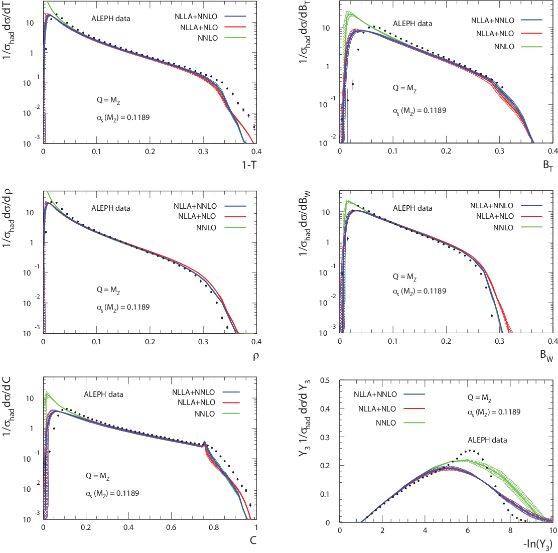
The parton-level fixed order NNLO and matched NLLA+NLO and NLLA+NNLO predictions are compared to hadron-level data taken by the ALEPH experiment [1] in Figure 3. The description of the hadron-level data improves between parton-level NLLA+NLO and parton-level NLLA+NNLO, especially in the three-jet region for most event shapes. The behaviour in the two-jet region is described better by the resummed predictions than by the fixed order NNLO, although the agreement is far from perfect. This discrepancy was observed already in earlier studies based on NLLA+NLO. It can in part be attributed to hadronisation corrections, which become large in the approach to the two-jet limit. A very recent study of logarithmic corrections beyond NLLA for the thrust distribution [29] also shows that subleading logarithms in the two-jet region can account for about half of this discrepancy.

A precise extraction of $\alpha_{s}$ from event shape data will require the inclusion of hadronisation corrections and of quark mass effects (at least to NLO [33]), as done already in the fixed order NNLO study [32]. It can be anticipated that inclusion of the matched NLLA+NNLO corrections results in a further improvement of the extraction of $\alpha_{s}$ from event shape data over results obtained previously at NLLA+NLO as well as at NNLO. The principal shortcomings of the up-to-now default NLLA+NLO studies were the substantial renormalisation scale uncertainty and the sizable scatter of values of $\alpha_{s}$ obtained from different shape variables. It was observed recently, that a fixed-order NNLO extraction [32] reduces the renormalisation scale uncertainty by a factor 1.3 compared to NLLA+NLO and eliminates the scatter between different observables. It will be very interesting to see the impact of the matched NLLA+NNLO calculation on the extraction of $\alpha_{s}$. We will address this issue in a future study.

A routine implementing the matching for all event shapes discussed here can be obtained upon request from the authors.

References

• [1] D. Buskulic et al. [ALEPH Collaboration], Z. Phys. C 73 (1997) 409;
A. Heister et al. [ALEPH Collaboration], Eur. Phys. J. C 35 (2004) 457.
• [2] P. Abreu et al. [DELPHI Collaboration], Phys. Lett. B 456 (1999) 322;
J. Abdallah et al. [DELPHI Collaboration], Eur. Phys. J. C 29 (2003) 285 [hep-ex/0307048];
J. Abdallah et al. [DELPHI Collaboration], Eur. Phys. J. C 37 (2004) 1 [hep-ex/0406011].
• [3] M. Acciarri et al. [L3 Collaboration], Phys. Lett. B 371 (1996) 137;
M. Acciarri et al. [L3 Collaboration], Phys. Lett. B 404 (1997) 390;
M. Acciarri et al. [L3 Collaboration], Phys. Lett. B 444 (1998) 569;
P. Achard et al. [L3 Collaboration], Phys. Lett. B 536 (2002) 217 [hep-ex/0206052];
P. Achard et al. [L3 Collaboration], Phys. Rept. 399 (2004) 71 [hep-ex/0406049].
• [4] P. D. Acton et al. [OPAL Collaboration], Z. Phys. C 59 (1993) 1;
G. Alexander et al. [OPAL Collaboration], Z. Phys. C 72 (1996) 191;
K. Ackerstaff et al. [OPAL Collaboration], Z. Phys. C 75 (1997) 193;
G. Abbiendi et al. [OPAL Collaboration], Eur. Phys. J. C 16 (2000) 185 [hep-ex/0002012];
G. Abbiendi et al. [OPAL Collaboration], Eur. Phys. J. C 40 (2005) 287 [hep-ex/0503051].
• [5] S. Brandt, C. Peyrou, R. Sosnowski and A. Wroblewski, Phys. Lett. 12 (1964) 57;
E. Farhi, Phys. Rev. Lett. 39 (1977) 1587.
• [6] L. Clavelli and D. Wyler, Phys. Lett. B 103 (1981) 383.
• [7] P.E.L. Rakow and B.R. Webber, Nucl. Phys. B 191 (1981) 63.
• [8] G. Parisi, Phys. Lett. B 74 (1978) 65;
J.F. Donoghue, F.E. Low and S.Y. Pi, Phys. Rev. D 20 (1979) 2759.
• [9] S. Catani, Y.L. Dokshitzer, M. Olsson, G. Turnock and B.R. Webber, Phys. Lett. B 269 (1991) 432;
N. Brown and W.J. Stirling, Phys. Lett. B 252 (1990) 657; Z. Phys. C 53 (1992) 629;
W.J. Stirling et al., Proceedings of the Durham Workshop, J. Phys. G17 (1991) 1567;
S. Bethke, Z. Kunszt, D.E. Soper and W.J. Stirling, Nucl. Phys. B 370 (1992) 310 [Erratum-ibid. B 523 (1998) 681].
• [10] R.W.L. Jones, M. Ford, G.P. Salam, H. Stenzel and D. Wicke, JHEP 0312 (2003) 007 [hep-ph/0312016].
• [11] S. Catani, L. Trentadue, G. Turnock and B.R. Webber, Nucl. Phys. B 407 (1993) 3.
• [12] R.K. Ellis, D.A. Ross and A.E. Terrano, Nucl. Phys. B 178 (1981) 421.
• [13] Z. Kunszt, Phys. Lett. B 99 (1981) 429;
J.A.M. Vermaseren, K.J.F. Gaemers and S.J. Oldham, Nucl. Phys. B 187 (1981) 301;
K. Fabricius, I. Schmitt, G. Kramer and G. Schierholz, Z. Phys. C 11 (1981) 315.
• [14] Z. Kunszt and P. Nason, in Z Physics at LEP 1, CERN Yellow Report 89-08, Vol. 1, p. 373;
W. T. Giele and E.W.N. Glover, Phys. Rev. D 46 (1992) 1980;
S. Catani and M. H. Seymour, Phys. Lett. B 378 (1996) 287 [hep-ph/9602277].
• [15] A. Gehrmann-De Ridder, T. Gehrmann, E.W.N. Glover and G. Heinrich, Phys. Rev. Lett. 99 (2007) 132002 [arXiv:0707.1285].
• [16] A. Gehrmann-De Ridder, T. Gehrmann, E.W.N. Glover and G. Heinrich, JHEP 0711 (2007) 058 [arXiv:0710.0346].
• [17] A. Gehrmann-De Ridder, T. Gehrmann, E.W.N. Glover and G. Heinrich, JHEP 0712 (2007) 094 [arXiv:0711.4711].
• [18] A. Gehrmann-De Ridder, T. Gehrmann, E.W.N. Glover and G. Heinrich, Phys. Rev. Lett. 100 (2008) 172001 [arXiv:0802.0813.]
• [19] S. Catani, G. Turnock, B.R. Webber and L. Trentadue, Phys. Lett. B 263 (1991) 491.
• [20] S. Catani, G. Turnock and B.R. Webber, Phys. Lett. B 272 (1991) 368;
E. Gardi and J. Rathsman, Nucl. Phys. B 638 (2002) 243 [hep-ph/0201019].
• [21] S. Catani, G. Turnock and B.R. Webber, Phys. Lett. B 295 (1992) 269.
• [22] Y.L. Dokshitzer, A. Lucenti, G. Marchesini and G.P. Salam, JHEP 9801 (1998) 011 [hep-ph/9801324].
• [23] S. Catani and B. R. Webber, Phys. Lett. B 427 (1998) 377 [hep-ph/9801350];
E. Gardi and L. Magnea, JHEP 0308 (2003) 030 [hep-ph/0306094].
• [24] S. Catani and B.R. Webber, JHEP 9710 (1997) 005 [hep-ph/9710333].
• [25] A. Banfi, G.P. Salam and G. Zanderighi, JHEP 0201 (2002) 018 [hep-ph/0112156].
• [26] A. Banfi, G.P. Salam and G. Zanderighi, JHEP 0503 (2005) 073 [hep-ph/0407286].
• [27] D. de Florian and M. Grazzini, Nucl. Phys. B 704 (2005) 387 [hep-ph/0407241].
• [28] S. Fleming, A. H. Hoang, S. Mantry and I. W. Stewart, Phys. Rev. D 77 (2008) 074010 [arXiv:hep-ph/0703207];
S. Fleming, A. H. Hoang, S. Mantry and I. W. Stewart, arXiv:0711.2079;
M.D. Schwartz, Phys. Rev. D 77 (2008) 014026 [arXiv:0709.2709];
C.W. Bauer, S.P. Fleming, C. Lee and G. Sterman, arXiv:0801.4569.
• [29] T. Becher and M.D. Schwartz, arXiv:0803.0342.
• [30] A. Banfi and G. Zanderighi, private communication.
• [31] S. Bethke, Prog. Part. Nucl. Phys. 58 (2007) 351 [hep-ex/0606035].
• [32] G. Dissertori, A. Gehrmann-De Ridder, T. Gehrmann, E.W.N. Glover, G. Heinrich and H. Stenzel, JHEP 0802 (2008) 040 [arXiv:0712.0327].
• [33] W. Bernreuther, A. Brandenburg and P. Uwer, Phys. Rev. Lett. 79 (1997) 189 [hep-ph/9703305];
A. Brandenburg and P. Uwer, Nucl. Phys. B 515 (1998) 279 [hep-ph/9708350];
G. Rodrigo, A. Santamaria and M. S. Bilenky, Phys. Rev. Lett. 79 (1997) 193 [hep-ph/9703358];
P. Nason and C. Oleari, Nucl. Phys. B 521 (1998) 237 [hep-ph/9709360].
Thrust: y=τ=1−Ty=\tau=1-T and CC-parameter: y=C/6y=C/6
G11=3​CFG12=−2​CFG22=136​CF​(−169​CA+22​NF+12​(CA−4​CF)​π2)G23=13​CF​(−11​CA+2​NF)G33=1108​CF​[−612​CA2+180​CA​NF+108​CF​NF+(11​CA−2​NF)​(−235​CA+34​NF+12​(CA−6​CF)​π2)+2304​CF2​ζ​(3)]G34=−7108​CF​(11​CA−2​NF)2\begin{array}[]{ccl}\hline\cr\\[-4.2194pt] G_{11}&=&3\,C_{F}\\[3.41432pt] G_{12}&=&-2\,C_{F}\\[3.41432pt] G_{22}&=&\frac{1}{36}\,C_{F}\left(-169C_{A}+22N_{F}+12\left(C_{A}-4C_{F}\right)\pi^{2}\right)\\[3.41432pt] G_{23}&=&\frac{1}{3}\,C_{F}\left(-11C_{A}+2N_{F}\right)\\[3.41432pt] G_{33}&=&\frac{1}{108}\,C_{F}\left[-612C_{A}^{2}+180C_{A}N_{F}+108C_{F}N_{F}+\left(11C_{A}-2N_{F}\right)\left(-235\,C_{A}+34\,N_{F}+12\left(C_{A}-6\,C_{F}\right)\pi^{2}\right)+2304\,C_{F}^{2}\zeta(3)\right]\\[3.41432pt] G_{34}&=&-\frac{7}{108}C_{F}\left(11\,C_{A}-2\,N_{F}\right)^{2}\\[3.41432pt] \hline\cr\end{array}
Heavy jet mass: y=ρy=\rho
G11=3​CFG12=−2​CFG22=136​CF​(−169​CA+22​NF+12​(CA−2​CF)​π2)G23=13​CF​(−11​CA+2​NF)G33=1108​CF​[−612​CA2+180​CA​NF+108​CF​NF+(11​CA−2​NF)​(−235​CA+34​NF+12​(CA−3​CF)​π2)+576​CF2​ζ​(3)]G34=−7108​CF​(11​CA−2​NF)2\begin{array}[]{ccl}\hline\cr\\[-4.2194pt] G_{11}&=&3\,C_{F}\\[3.41432pt] G_{12}&=&-2\,C_{F}\\[3.41432pt] G_{22}&=&\frac{1}{36}\,C_{F}\left(-169C_{A}+22N_{F}+12\left(C_{A}-2C_{F}\right)\pi^{2}\right)\\[3.41432pt] G_{23}&=&\frac{1}{3}\,C_{F}\left(-11C_{A}+2N_{F}\right)\\[3.41432pt] G_{33}&=&\frac{1}{108}\,C_{F}\left[-612C_{A}^{2}+180C_{A}N_{F}+108C_{F}N_{F}+\left(11C_{A}-2N_{F}\right)\left(-235\,C_{A}+34\,N_{F}+12\left(C_{A}-3\,C_{F}\right)\pi^{2}\right)+576\,C_{F}^{2}\zeta(3)\right]\\[3.41432pt] G_{34}&=&-\frac{7}{108}C_{F}\left(11\,C_{A}-2\,N_{F}\right)^{2}\\[3.41432pt] \hline\cr\end{array}
Total jet broadening: y=BTy=B_{T}
G11=6​CFG12=−4​CFG22=−19​CF​(35​CA−2​NF−6​CA​π2+24​CF​π2+288​CF​ln2​2)G23=−89​CF​(11​CA−2​NF)G33=281​CF​(−2471​CA2+760​CA​NF+108​CF​NF−44​NF2+132​CA2​π2−792​CA​CF​π2−24​CA​NF​π2+144​CF​NF​π2CLOSEOPEN+864​CF2​π2​ln​2−9504​CA​CF​ln2​2+1728​CF​NF​ln2​2−5184​CF2​ln3​2+2376​CF2​ζ​(3))G34=−29​CF​(11​CA−2​NF)2\begin{array}[]{ccl}\hline\cr\\[-4.2194pt] G_{11}&=&6C_{F}\\[3.41432pt] G_{12}&=&-4C_{F}\\[3.41432pt] G_{22}&=&-\frac{1}{9}C_{F}\left(35C_{A}-2N_{F}-6C_{A}\pi^{2}+24C_{F}\pi^{2}+288C_{F}\,\hbox{ln}^{2}2\right)\\[3.41432pt] G_{23}&=&-\frac{8}{9}C_{F}\left(11C_{A}-2N_{F}\right)\\[3.41432pt] G_{33}&=&\frac{2}{81}C_{F}\left(-2471C_{A}^{2}+760C_{A}N_{F}+108C_{F}N_{F}-44N_{F}^{2}+132C_{A}^{2}\pi^{2}-792C_{A}C_{F}\pi^{2}-24C_{A}N_{F}\pi^{2}+144C_{F}N_{F}\pi^{2}\right.\\ &&\hskip 16.38895pt\hskip 8.19447pt\left.+864C_{F}^{2}\pi^{2}\hbox{ln}2-9504C_{A}C_{F}\hbox{ln}^{2}2+1728C_{F}N_{F}\hbox{ln}^{2}2-5184C_{F}^{2}\hbox{ln}^{3}2+2376C_{F}^{2}\zeta\left(3\right)\right)\\[3.41432pt] G_{34}&=&-\frac{2}{9}C_{F}\left(11C_{A}-2N_{F}\right)^{2}\\[3.41432pt] \hline\cr\end{array}
Wide jet broadening: y=BWy=B_{W}
G11=6​CFG12=−4​CFG22=−19​CF​(35​CA−2​NF−6​CA​π2+288​CF​ln2​2)G23=−89​CF​(11​CA−2​NF)G33=281​CF​(−2471​CA2+760​CA​NF+108​CF​NF−44​NF2+132​CA2​π2−24​CA​NF​π2+864​CF2​π2​ln​2−9504​CA​CF​ln2​2CLOSEOPEN+1728​CF​NF​ln2​2−5184​CF2​ln3​2−2808​CF2​ζ​(3))G34=−29​CF​(11​CA−2​NF)2\begin{array}[]{ccl}\hline\cr\\[-4.2194pt] G_{11}&=&6C_{F}\\[3.41432pt] G_{12}&=&-4C_{F}\\[3.41432pt] G_{22}&=&-\frac{1}{9}C_{F}\left(35C_{A}-2N_{F}-6C_{A}\pi^{2}+288C_{F}\,\hbox{ln}^{2}2\right)\\[3.41432pt] G_{23}&=&-\frac{8}{9}C_{F}\left(11C_{A}-2N_{F}\right)\\[3.41432pt] G_{33}&=&\frac{2}{81}C_{F}\left(-2471C_{A}^{2}+760C_{A}N_{F}+108C_{F}N_{F}-44N_{F}^{2}+132C_{A}^{2}\pi^{2}-24C_{A}N_{F}\pi^{2}+864C_{F}^{2}\pi^{2}\hbox{ln}2-9504C_{A}C_{F}\hbox{ln}^{2}2\right.\\ &&\hskip 16.38895pt\hskip 8.19447pt\left.+1728C_{F}N_{F}\hbox{ln}^{2}2-5184C_{F}^{2}\hbox{ln}^{3}2-2808C_{F}^{2}\zeta\left(3\right)\right)\\[3.41432pt] G_{34}&=&-\frac{2}{9}C_{F}\left(11C_{A}-2N_{F}\right)^{2}\\[3.41432pt] \hline\cr\end{array}
Two-to-three jet transition in Durham algorithm: y=Y3y=Y_{3}
G11=3​CFG12=−CFG22=136​CF​(−35​CA+144​CF​ℱ2+2​NF+6​CA​π2)G23=−19​CF​(11​CA−2​NF)G33=1324​CF​(−2471​CA2+4752​CA​CF​ℱ2+2592​CF2​ℱ3+760​CA​NF+108​CF​NF−864​CF​ℱ2​NF−44​NF2+132​CA2​π2CLOSEOPEN−24​CA​NF​π2)G34=−172​CF​(11​CA−2​NF)2\begin{array}[]{ccl}\hline\cr\\[-4.2194pt] G_{11}&=&3C_{F}\\[3.41432pt] G_{12}&=&-C_{F}\\[3.41432pt] G_{22}&=&\frac{1}{36}C_{F}\left(-35C_{A}+144C_{F}\mathcal{F}_{2}+2N_{F}+6C_{A}\pi^{2}\right)\\[3.41432pt] G_{23}&=&-\frac{1}{9}C_{F}\left(11C_{A}-2N_{F}\right)\\[3.41432pt] G_{33}&=&\frac{1}{324}C_{F}\left(-2471C_{A}^{2}+4752C_{A}C_{F}\mathcal{F}_{2}+2592C_{F}^{2}\mathcal{F}_{3}+760C_{A}N_{F}+108C_{F}N_{F}-864C_{F}\mathcal{F}_{2}N_{F}-44N_{F}^{2}+132C_{A}^{2}\pi^{2}\right.\\ &&\left.-24C_{A}N_{F}\pi^{2}\right)\\[3.41432pt] G_{34}&=&-\frac{1}{72}C_{F}\left(11C_{A}-2N_{F}\right)^{2}\\[3.41432pt] \hline\cr\end{array}