Joint effects of nutrients and contaminants on the dynamics of a food chain in marine ecosystems
Abstract
We analyze the joint effect of contaminants and nutrient loading on population dynamics of marine food chains by means of bifurcation analysis. Contaminant toxicity is assumed to alter mortality of some species with a sigmoidal dose-response relationship. A generic effect of pollutants is to delay transitions to complex dynamical states towards higher nutrient load values, but more counterintuitive consequences arising from indirect effects are described. In particular, the top predator seems to be the species more affected by pollutants, even when contaminant is toxic only to lower trophic levels.
Keywords:
Contaminants , nutrient load , food chain , bifurcation analysis , indirect effects1 Introduction
Marine waters and in particular coastal waters are increasingly exposed to anthropogenic pressures represented not only by the growing input of nutrients and contaminants related to urban, agricultural and industrial activities, but also by the exploitation of coastal areas for aquaculture, fishing and tourism. Since the resources of the coastal zone are exploited by different stakeholders, it is essential to improve our knowledge on the ecosystem’s vulnerability to stressors and protect those areas through a sensible management.
The interaction of pollutants and nutrients on aquatic ecosystems is difficult to evaluate, since many direct and indirect effects have to be considered. Contaminants can have instantaneous effects, such as massive killings after an accidental contaminant release. Other toxic effects, such as genotoxicity and reproductive failure are less evident and they act on a longer time-scale; however, they represent an important risk for the ecosystem. Furthermore, if the contaminant is lipophilic, bioaccumulation should be considered. On the other hand, an increase of the nutrient load can have the direct effect of raising the primary production at the bottom of the food chain and consequently increasing the concentration of the organic matter in the system. But a higher concentration of organic matter can affect the bioavailability of the contaminants and therefore the fate of pollutants in the aquatic environment and their effects on the impacted ecosystem [1].
Thus, contaminants affect aquatic ecosystems through direct and indirect effects [2], from acute and/or chronic toxicity on sensitive species to disruption in the food web structure. Some species might be more sensitive than others to a particular chemical, but since the different populations are linked to each other by competition and predation, species which are not directly stressed may respond indirectly [2]. Within a food web, community-level relations arise from unobservable indirect pathways. These relations may give rise to indirectly mediated relations, mutualism and competition [3]. In some cases environmental perturbations alter substantially the dynamics or the structure of coastal ecosystems and the effect may produce the occurrence of a trophic cascade and eventually the extinction of some species [4]. A better understanding of the relative importance of top-down (e.g. overfishing) versus bottom-up (e.g. increased nutrient input causing eutrophication) controls is essential and can only be achieved through modelling [5].
Sudden regime shifts and ecosystem collapses are likely to occur in stressed ecosystems. Catastrophic regime shifts have been related to alternative stable states which can be linked to a critical threshold in such a way that a gradual increase of one driver has little influence until a certain value is reached at which a large shift occurs that is difficult to reverse [6, 7]. The shape of ecotoxicological dose-response curves [8], showing a sharp increase in the effect of toxic substances above a critical value, facilitates the occurrence of regime shifts under pollutant pressure.
In this study we consider the combined effects of contaminant substances and nutrient load in the framework of a simple tritrophic food chain model. We restrict our study to contaminants, such as s-triazines, which affect the mortality in particular trophic levels, but which do not bioaccumulate in time nor along the food chain. When studying the dynamics of simple food chain and food web models, it is also important to bear in mind that the response might depend on the complexity of the represented system. Chaotic dynamics, for example, seems to be more frequent in simple ecosystem models or in models with a high number of trophic levels [9]. Thus, we will focus only on the first qualitative changes of behaviour occurring when increasing nutrients from low values, and how this is changed by pollutants, and not on the complex sequences of chaotic states which may occur at high nutrient availability, whose details are more affected by the trophic structure of the model.
Since we do not include any microbial recycling loop, sediment or oxygen dynamics, or shading effects, complex eutrophication behaviour typical of coastal ecosystems [10], e.g. anoxic crises, alteration of nutrient cycling, macroalgal blooms, etc, will not occur in our model. We rather concentrate on the simplest scenarios occurring during enrichment and its modification by contaminants, discussing particularly the indirect effects which lead to counterintuitive behaviour.
2 Model formulation
We consider [11, 12, 13] Canale’s chemostat model (CC), which is an extension of the tri-trophic food-chain Rosenzweig-MacArtur model (RMA) that has been extensively studied in theoretical ecology [14, 15, 16, 17, 18, 19, 20, 21]. This model was previously used to analyze the dynamics of a food chain consisting of bacteria living on glucose, ciliates and carnivorous ciliates [11, 12], but can be adapted to represent an aquatic food chain with a constant nutrient input. The CC model is similar to the RMA model, but there is an additional equation representing the input of nutrient, and it considers the losses due to the flushing rate:
| (1) | |||||
| (2) | |||||
| (3) | |||||
| (4) |
In this study the variables , , , represent the nitrogen concentration in the different compartments of the system (nutrient, phytoplankton, zooplankton and fish, which will be also denoted with the alternative names of nutrient, prey, predator, and top-predator, respectively) expressed in units of . Our default parameters (see Table 1) are from [22], as used in the aquatic food chain model presented in [23]. Apart from unessential scaling differences, most of the parameters are of the same order as in [20, 13], except that we use larger mortality values and, accordingly, smaller flushing rates to avoid complete extinction of the ecosystem. Our base mortalities and the rest of parameters are consistent with the ones used in the pelagic ecosystem model in [24] which, as discussed in that reference, are adequate for the oligotrophic subtropical ocean. is the nutrient load or nutrient input into the system. is a flow rate quantifying water renewal in the system, which affects the species through the flushing rates (). are the specific mortalities, half saturation constants for the Holling type-II predation functions, are maximum predation rates, and efficiencies. We note that the following condition should be satisfied by the equation parameters:
| (5) |
since this “avoids the case where predator and top-predator cannot survive, even when their food is infinitely abundant” [25]. Contaminant toxicity is incorporated in our model by an increase in mortality. We consider three different scenarios in each of which the contaminant affects the mortality of only one of the compartments:
| (6) |
, and labels the three trophic levels: prey, predator and top-predator, is the dimensionless concentration of the contaminant affecting the level , normalized in such a way that for the toxicity achieves half its maximum impact on mortality, and a sigmoidal function (Fig. 1) has been used to model the mortality increase from a baseline value, , to the maximum mortality, , attained at large contaminant concentrations. This represents typically the shape of the dose-response curves found when assessing toxic effects of chemical on biological populations [8]. The values of and used are written in Table 2. Other works that have studied bifurcations due to mortality changes in the CC model [13] have normally considered a linear increase. Considering a sigmoidal response allows the identification of the range of mortality values which are to be expected in the presence of a given contaminant, and thus permits to focus in such range. But once the relevant interval is identified the bifurcation behavior can be studied as a function of the mortalities . This was done in Ref. [13] with emphasis in steady coexistence solutions. Here, in addition to exploring a different set of base parameters and to focusing in the mortality range implied by the contaminant characteristics in Table 2, we also perform continuations of cyclic solutions and find some period doubling bifurcations which would eventually lead to chaos.
3 Steady states
This system presents the following set of fixed points: The nutrient-only state (Nu):
| (7) | |||||
The nutrient-phytoplankton state (NP):
| (8) | |||||
There are two solutions (NPZ) characterized by the absence of the top predator:
| (9) | |||||
but only the one with the positive sign of the square root is positive definite.
Finally, there are three internal fixed points (NPZF), in which all species occur at positive densities. From the equation for , (1), an equation for as a function of is obtained. Introducing it into (2) together with the expression for which is obtained from (4), we get the following equation for :
| (10) |
where
| (11) | |||||
The values of the remaining variables at the three internal fixed point solutions can be written in terms of and of the three values of obtained from the cubic (10):
| (12) | |||||
It turns out that only one of the three fixed point solutions is positive for the parameter values in Table 1.
The above are all the biologically relevant fixed points. There are four additional mathematical steady state solutions, but some populations take negative values on them.
4 Stability and bifurcation analysis
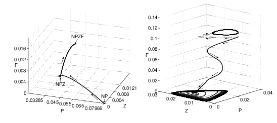
We have analyzed the dynamics of the CC food-chain models for several parameter values by direct numerical integration of the model equations, and by bifurcation analysis carried on with the software AUTO [26]. Background on the different types of bifurcations can be found in [27, 28]. We consider only bifurcations of positive solutions and, as stated in the introduction, we find but we do not describe in detail the routes to chaotic behaviour occurring at high nutrient load. For low and intermediate nutrient load we find that the relevant attractors are the fixed points described above, and also two limit cycles, one involving the variables , and , lying on the hyperplane, and another one in which all the species are present. These attractors are represented in Fig.2.
4.1 The non-contaminant case
First, we consider system behaviour for the case of mortalities at their base values, i.e. in the absence of contaminants. This will serve as a reference for later inclusion of contaminants. Fig.3 shows the sequence of bifurcations when increasing the nutrient input . For very low input, only nutrients are present in the system (solution (7)). When , with
| (13) |
phytoplankton becomes positive in a transcritical bifurcation (which we call TB1) at which the NP state (8) becomes stable. Since is very small, this bifurcation can not be clearly seen in Fig. 3. From this value on, further enrichment leads to a linear increase of phytoplankton (8), until a second transcritical bifurcation, TB2, at which zooplankton becomes positive and the NPZ solution (9) becomes stable. It happens at
| (14) |
where is the expression for in the solution, (9). From this point the zooplankton starts increasing (keeping phytoplankton concentration at a constant value) until a new bifurcation TB3 occurs, at which the fish concentration starts to grow from zero while zooplankton remains constant, phytoplankton increases, and nutrients decrease (this is the positive interior solution NPZF, Eq. (12)). The value of is given implicitly by:
| (15) |
where is the expression for in the solution, (9).
We note here one of the first counterintuitive indirect effects present in the food-chain dynamics: In the NPZF solution, increase of nutrient input leads to decrease in nutrient concentration (see Fig. 3). The reason is the top-down control that the higher predator begins to impose on zooplankton, leading to positive and negative regulation on the compartments situated one or two trophic levels below , respectively.
Shortly after becoming unstable at TB3, the fixed point NPZ experiences a Hopf bifurcation (HB1) which leads to a limit cycle on the NPZ hyperplane. Since the whole hyperplane has become unstable before this bifurcation occurs, this cycle has no direct impact on long time dynamics, although it can affect transients, and it will become relevant when adding contaminants. The steady state coexistence of the three species at the NPZF fixed point remains stable until a new Hopf bifurcation HB2 occurs at which the fixed point becomes unstable and oscillations involving the three species and the nutrients (Fig. 2) occur. The destabilization of steady state coexistence by the appearance of oscillations, which could facilitate extinctions if the amplitude of oscillation is sufficiently large, is the well known “paradox of enrichment”, first mathematically described by Rosenzweig [29]. A good overview of the studies connected with this issue can be found in the paper [30]. See also [31, 32, 33, 34].
Gragnani et al.[20] demonstrated that the dynamics of Canale’s model for increasing nutrient supply is qualitatively similar to the one of the RMA model. After the stationary and cyclic states described above, chaotic behaviour followed by a different cyclic behaviour with higher frequency are found. Also, the maximal average density of top-predator is attained at the threshold between chaotic and high frequency cyclic behaviour. We do not describe these states further but concentrate on the modifications arising from toxic effects of contaminants on the dynamics, for small and moderate nutrient loading.
4.2 Contaminant toxic to phytoplankton
We now introduce contaminant . It increases the mortality of phytoplankton according to expression (6) for . The main bifurcations are shown in the 2-parameter bifurcation diagram of Fig. 4 as a function of and (with values of also indicated). Expressions for the bifurcation lines TB1, TB2 and TB3 as a function of and can be obtained simply by replacing the mortality (6) into the corresponding expressions (13), (14), and (15), respectively. The same can be done numerically for the Hopf bifurcation lines HB1 and HB2. Because of the sigmoidal effect of the contaminant (6), its impact is mild for , and it will saturate for . Thus, in both limits the bifurcation lines would become parallel to the axis if plotted in terms of and . The interesting behaviour is for intermediate values of , to which most of Fig. 4 pertains. In this range the bifurcation lines are displaced towards higher values of . That is, the first effect of the contaminant is to stabilize the simplest solutions, the ones which are stable at lower nutrient load, delaying until higher nutrient loads the transitions to the most complex solutions.
But this stabilizing effect is different for the different solutions, and the most important qualitative change occurs at point M in Fig.4. It is a codimension-2 point at which the transcritical bifurcation TB3, involving the NPZ and the NPZF fixed points, and the Hopf bifurcation HB1 of the NPZ point, meet. A new Hopf bifurcation line of the NPZF equilibrium, HB3, emerges also from that point. The cycle created at HB3 consists in oscillations of all the four variables, similar to the cycle created at HB2. Other characteristics of the organizing center M is that the Hopf bifurcations change from subcritical to supercritical character across it, and also that a line (not shown) of saddle-node bifurcations of the cycles created at HB1 and HB3 emerges also from M. There are a number of additional structures in parameter space emerging from double-Hopf points, and transcritical bifurcations of cycles which we do not describe further here.
Despite the complexity of the above scenario, its effect on the bifurcation sequence when increasing nutrient level (up to moderate levels) in the presence of contaminant values beyond M is rather simple (see Fig.5): since the lines TB3 and HB1 have interchanged order, the Hopf bifurcation HB1 in which a stable limit cycle is created in the hyperplane occurs before the appearance of a positive NPZF equilibrium. As a consequence, fish remains absent from the system even at relatively high nutrient levels. This is one of the counterintuitive outcomes of indirect effects: adding a substance which is toxic for phytoplankton makes fish disappear, whereas the oscillating phytoplankton levels are indeed comparable with the ones at zero contaminant (see Fig. 5). As in the absence of a contaminant, period doublings and transition to chaos, which we have not analyzed in detail, occur with further increases in the value of .
A different view of the transitions can be given by describing the bifurcations occurring by increasing the contaminant concentration (or ) at constant . Fig. 6 shows that for an intermediate value of the nutrient load, . The NPZF fixed point is stable at low contaminant, but oscillations appear when crossing the HB3 lines. Very shortly after that, this limit cycle involving all species approaches the hyperplane until colliding with the cycle lying on that plane, which involves only the , , and species. At this transcritical bifurcation, this limit cycle from which fish is absent becomes stable and is the observed solution for larger or . As before, adding a substance which is toxic for the bottom of the trophic chain has the main effect of suppressing the top-predator.
4.3 Contaminant toxic to zooplankton
The 2-parameter bifurcation diagram of Fig. 7 displays the behaviour as a function of and the zooplankton mortality , as affected by contaminant . As before, the mortality expression (6) for can be inserted in the expressions (analytical or numerical) for the bifurcations TB1, TB2, TB3, HB1, and HB2 to elucidate the impact of the contaminant , acting on zooplankton, on the food chain dynamics. As in the case, the bifurcation lines become displaced to higher nutrient load values, so that the sequence of bifurcations of Fig. 3 becomes delayed to higher values of . In contrast with the case, the TB3 and HB1 lines do not cross, so that there are no further qualitative changes with respect to the case without contaminants (Fig. 3), at least up to moderate values of .
Another view of the consequences of Fig. 7 can be seen in Fig. 8, which shows the different regimes attained at a fixed intermediate value of () and increasing or . The most remarkable indirect effect is that, for (), zooplankton remains constant despite the increase of which is toxic to it. The net effect of in this range is to decrease the amount of fish until extinction. Only for contaminant kills zooplankton until extinction at ().
4.4 Contaminant toxic to fish
The simplest bifurcation lines are shown in Fig. 9 as a function of and , the fish mortality affected by contaminant . As in the cases before, bifurcations are delayed to higher values of when contaminant is present. As in the case, this delay is different for the different lines, resulting in a crossing of TB3 and HB1 in a codimension-2 point M, joining there also to a new Hopf bifurcation HB3 of the NPZF fixed point and other bifurcation lines (not shown). Additional structures emerging from other codimension-2 points, such as double-Hopf points are also present but we do not study them in detail. The qualitative behaviour when increasing at large or (Fig. 10) is similar to the case: there is a succession of N, NP and NPZ fixed points followed by a Hopf bifurcation which leads to oscillations of the , and variables, maintaining the absence of fish from the system. Only at relatively high nutrient values does the NPZF steady state become stable at the subcritical branch of the Hopf bifurcation HB3 before becoming unstable again at HB2. Two of the NPZF internal solutions (12), which, in contrast with the case, are positive here, collide at a limit point. In Fig. 9 the line of these points as a function of the and parameters is labelled as LP. The two solutions exist above that line, and cease to exist below. The sequence of bifurcations encountered when increasing or at constant intermediate values of is also similar to the case of Fig. 6 in that the NPZF stable fixed point becomes a cycle involving all the variables when HB3 is crossed, and in that it approaches the plane shortly afterwards. The details are, however, more complex because of the presence in phase space of additional unstable cycles.
5 Discussion and conclusion
Because of the assumed sigmoidal influence of contaminant on mortality, toxic effects on our food chain model have a distinct effect at low and at large concentrations, with rather fast transition behaviour in between.
At small and moderate contaminant concentrations the main effect is a displacement of the different bifurcations towards higher nutrient load values, so that transitions to states containing less active compartments, and states without oscillations, become relatively stabilized. Contaminants increase the stability of the food chain with respect to oscillations caused by increased nutrient input. A similar outcome has been observed in [35] for a food-chain model composed of a toxin producing phytoplankton, zooplankton and fish population. In that study chaotic dynamics can be stabilized by increasing the strength of toxic substance in the system.
For higher contaminant values, in most of the cases there is a reordering of the different transitions, giving rise to the appearance of new bifurcations which change qualitatively the sequence of states encountered by increasing nutrient input. The main effect, even in the cases in which such reordering does not occur (the case of contaminant), is that the top predator becomes the most depleted, being even brought to extinction. This strong impact of the contaminant on the higher predator occurs even in the cases in which the direct toxic effect is on lower trophic levels. It seems that the increased mortality at lower trophic levels becomes nearly compensated by a debilitation of top-down control exerted by higher predators. Obviously, the top predator can not benefit from this mechanism, thus becoming the most affected.
Extrapolation of the above findings for real ecosystems may be problematic, because of the much higher food web complexity found in nature. We believe however that the counterintuitive indirect effects described above should be kept in mind when analyzing the complex responses that ecosystems display to changes in external drivers such as nutrient load and pollutants, and that the detailed identification of them performed here can help to interpret some aspects of the behaviour of real ecosystems.
Acknowledgements
We acknowledge support from the European Commission through the integrated project THRESHOLDS (contract 003933) and from MEC (Spain) and FEDER, through project FISICOS (FIS2007-60327).
References
- [1] J. S. Gunnarsson, D.Broman, P. Jonsson, M. Olsson, R. Rosenberg, Interactions between eutrophication and contaminants: towards a new research concept for the European aquatic environment, AMBIO 24 (1995) 383–385.
- [2] J. Fleeger, K. Carman, R.M.Nisbet, Indirect effects of contaminants in aquatic ecosystems, The Science of the Total Environment 317 (2003) 207–233.
- [3] B. Fath, Network mutualism: Positive community-level relations in ecosystems, Ecological Modelling 208 (2007) 56–67.
- [4] J. Jackson, M. Kirby, W. Berger, K. Bjorndal, L. Botsford, B. Bourque, R. Bradbury, R. Cooke, J. Erlandson, J. Estes, T. Hughes, S. Kidwell, C. Lange, H. Lenihan, J. Pandolfi, C. Peterson, R. Steneck, M. Tegner, R. Warner, Historical overfishing and the recent collapse of coastal ecosystems, Science 293 (2001) 629–638.
- [5] G. Daskalov, Overfishing drives a trophic cascade in the Black Sea, Marine Ecology Progress Series 225 (2002) 53–63.
- [6] M. Scheffer, S. Carpenter, Catastrophic regime shifts in ecosystems: linking theory to observation, Trends in Ecology and Evolution 18 (2003) 648–656.
- [7] M. Scheffer, S. Carpenter, J. Foley, C. Folke, B. Walker, Catastrophic shifts in ecosystems, Nature 413 (2001) 591–596.
- [8] G. W. Suter II, Ecological Risk Assessment, Lewis Publishers, Boca Raton, Florida, 1993.
- [9] G. F. Fussmann, G. Heber, Food web complexity and chaotic population dynamics, Ecology Letters 5 (2002) 394–401.
- [10] J. Zaldívar, E. Cattaneo, M. Plus, C. N. Murray, G. Giordani, P. Viaroli, Long-term simulation of main biogeochemical events in a coastal lagoon: Sacca di Goro (Northern Adriatic Coast, Italy), Continental Shelf Research 23 (2003) 1847–1876.
- [11] M. P. Boer, B. W. Kooi, S. A. L. M. Kooijman, Food chain dynamics in the chemostat, Mathematical Biosciences 150 (1998) 43–62.
- [12] M. P. Boer, B. W. Kooi, S. A. L. M. Kooijman, Multiple attractor and boundary crises in a tri-trophic food chain, Mathematical Biosciences 169 (2001) 109–128.
- [13] C. R. Gwaltney, M. A. Stadtherr, Reliable computation of equilibrium states and bifurcations in ecological system analysis, Computers & Chemical Engineering 31 (2007) 993–1005.
- [14] A. Hastings, T. Powell, Chaos in a three-species food chain, Ecology 72(3) (1991) 896–903.
- [15] A. Klebanoff, A. Hastings, Chaos in three-species food chains, Journal of Mathematical Biology 32 (5) (1994) 427–451.
- [16] P. A. Abrams, J. D. Roth, The effects of enrichment of three-species food chains with non-linear functional responses, Ecology 75 (1994) 1118–1130.
- [17] K. McCann, P. Yodzis, Biological conditions for chaos in a three-species food chain, Ecology 75 (2) (1994) 561–564.
- [18] Y. Kuznetsov, S. Rinaldi, Remarks on food chain dynamics, Mathematical Biosciences 134 (1996) 1–33.
- [19] O. DeFeo, S. Rinaldi, Yield and dynamics of tritrophic food chains, The American Naturalist 150 (3) (1997) 328–345.
- [20] A. Gragnani, O. D. Feo, S. Rinaldi, Food chain dynamics in the chemostat: Relationships between mean yield and complex dynamics, Bulletin of Mathematical Biology 60 (1998) 703–719.
- [21] C. R. Gwaltney, M. P. Styczynsky, M. A. Stadtherr, Reliable computation of equilibrium states and bifurcations in food chain models, Computers & Chemical Engineering 28 (2004) 1981–1996.
- [22] S. E. Jorgensen (Ed.), Handbook of Ecological Parameters, Pergamon Press, 1979.
- [23] E. Mosekilde, Topics in Nonlinear Dynamics. Application to Physics, Biology and Economic Systems, World Scientific publishing, Singapore, 1998.
- [24] I. D. Lima, D. B. Olson, S. C. Doney, Intrinsic dynamics and stability properties of size-structured pelagic ecosystem models, Journal of Plankton Research 24 (6) (2002) 533–556.
- [25] Y. A. Kuznetsov, O. D. Feo, S. Rinaldi, Belyakov homoclinic bifurcations in a tritrophic food chain model, SIAM Journal on Applied Mathematics 62 (2001) 462–487.
- [26] E. J. Doedel, A. R. Champneys, T. F. Fairgrieve, Y. A. Kuznetsov, B. Sandstede, X. Wang, Auto 97: continuation and bifurcation software for ordinary differential equations, Technical report, Concordia University, Montreal, Canada (1997).
- [27] S. H. Strogatz, Nonlinear dynamics and chaos: With applications to Physics, Biology, Chemistry, and Engineering, Perseus Books group, Cambridge, Massachusetts, 2000.
- [28] J. Gugenheimer, P. Holmes, Nonlinear oscillations, dynamical systems and bifurcations of vector fields, Vol. 42, Applied mathematical sciences, Springer-Verlag, New York Inc, 1993.
- [29] M. L. Rosenzweig, Paradox of enrichment: destabilization of exploitation ecosystems in ecological time, Science 171 (1971) 385–387.
- [30] C. X. J. Jensen, L. R. Ginzburg, Paradoxes or theoretical failure? The jury is still out, Ecological Modelling 188 (2005) 3–14.
- [31] G. F. Fussmann, S. P. Ellner, K. W. Sherzer, N. G. H. Jr, Crossing the Hopf bifurcation in a live predator-prey system, Science 290 (2000) 1358–1360.
- [32] K. W. Shertzer, S. P. Ellner, G. F. Fussmann, N. G. H. Jr, Predator-prey cycles in an aquatic microcosm: testing hypotheses of mechanism, Journal of Animal Ecology 71 (2002) 802–815.
- [33] T. Bell, The ecological consequences of unpalatable prey: phytoplankton response to nutrient and predator additions, Oikos 99 (2002) 59–68.
- [34] K. L. Kirk, Enrichment can stabilize population dynamics: autotoxins and density dependence, Ecology 79 (7) (1998) 2456–2462.
- [35] R. K. Upadhayay, J. Chattopadhayay, Chaos to order: role of toxin producing phytoplankton in aquatic systems, Nonlinear analysis: modeling and control 10 (4) (2005) 383–396.
| Parameters | value | Units | |
|---|---|---|---|
| Nutrient input | mg N/l | ||
| Inflow/outflow rate | |||
| Max predation rate | |||
| Half saturation cont | mg N/l | ||
| mg N/l | |||
| mg N/l | |||
| Efficiency | - | ||
| - | |||
| - | |||
| Mortality(base values) | |||
| Flushing rate | |||
| 1 (prey) | 0.1 | 0.5 |
|---|---|---|
| 2 (predator) | 0.1 | 0.3 |
| 3 (top-predator) | 0.015 | 0.015 |
Figure captions
Fig.1. Sigmoidal response of mortality to the concentration of the toxic contaminant, according to Eq. (6).
Fig.2. (a). Projection on the PZF subspace of a trajectory which starts close to the NP fixed point, approaches the NPZ one, and finally is attracted by the NPZF fixed point. , , and . This shows the approximate location of these points and that only the NPZF one is stable for these parameter values. (b) Cyclic behaviour: Thick line is a trajectory leading to an attracting limit cycle on the NPZ hyperplane for , , and ; dotted line is a trajectory attracted by the limit cycle involving all the variables for , , and .
Fig.3. Bifurcation diagrams of the four variables as a function of nutrient input parameter in the absence of contaminants. Thick lines and full symbols denote stable fixed points and maxima and minima of stable cycles, respectively, and thin lines and open symbols, unstable ones. The names of the fixed points are indicated. The relevant bifurcations (described in the main text) occur at , , , , and , locations which are indicated by arrows.
Fig.4. Some of the bifurcations occurring as a function of nutrient input and the phytoplankton mortality , in the range of values determined by the presence of contaminant affecting phytoplankton. Values of are also indicated in the upper horizontal axis. The names of the bifurcation lines are indicated (for the case of the Hopf lines HB1, HB2 and HB3, the name of the fixed point involved in the bifurcation is shown in parenthesis). Crossing the continuous lines involves a qualitative change for the state attained by the system. Inside regions surrounded by continuous lines, the name of the relevant stable fixed point is shown inside grey squares. Crossing the discontinuous bifurcation lines does not involve a change in the stable state (because, e.g., they correspond to bifurcations of already unstable states). Immediately above the HB2 line, a limit cycle involving all the species is the relevant attractor for low values of (or ). The limit cycle on the hyperplane is the relevant attractor above the HB1 line for large . Additional bifurcations (not shown) occur in other regions of the open areas above HB1 and HB2. M is a codimension-2 point described in the main text. The dotted region identifies areas where chaotic solutions have been found.
Fig.5. Bifurcation diagrams of the four variables as a function of nutrient input parameter , at a constant high value of the contaminant affecting phytoplankton, (). Thick lines and full symbols denote stable fixed points and maxima and minima of stable cycles, respectively, and thin lines and open symbols, unstable ones. The names of the fixed points are shown. The bifurcation points are identified by arrows. PD is a period doubling bifurcation.
Fig.6. Bifurcation diagrams of the four variables as a function of , affected by contaminant , at constant nutrient input . Thick lines and full symbols denote stable fixed points and maxima and minima of stable cycles, respectively, and thin lines and open symbols, unstable ones. BP is a transcritical bifurcation of cycles. The name of the fixed points is shown. The bifurcation points are identified by arrows.
Fig. 7. Some of the bifurcations occurring as a function of nutrient input and zooplankton mortality , in the range of values determined by the presence of contaminant affecting zooplankton. Values of are also indicated in the upper horizontal axis. Names of fixed points and bifurcation lines are as in Fig. 4, as well as the meaning of continuous and discontinuous lines. Immediately above the HB2 line, the relevant attractor is a limit cycle involving all the species. Additional bifurcations (not shown) occur at higher values of . The dotted region identifies areas where chaotic solutions have been found.
Fig. 8. Bifurcation diagrams of the four variables as a function of , affected by contaminant , for a constant nutrient load . Thick lines denote stable fixed and thin lines and open symbols, unstable fixed points and maxima and minima of unstable cycles. The names of the fixed points are shown. The bifurcation points are identified by arrows.
Fig. 9. Some of the bifurcations occurring as a function of nutrient input and fish mortality , in the range of values determined by the presence of contaminant affecting fish. Values of are also indicated in the upper horizontal axis. Names of fixed points and bifurcation lines are as in Fig. 4, as well as the meaning of continuous and discontinuous lines. Immediately above the HB2 line, the relevant attractor is a limit cycle involving all the species. Additional bifurcations (not shown) occur at higher values of . The dotted region identifies areas where chaotic solutions have been found. There is a region of the area labelled as NPZF in which this stable fixed point coexists with a stable limit cycle on the hyperplane.
Fig. 10. Bifurcation diagrams of the four variables as a function of nutrient input rate parameter for a high value of the contaminant affecting fish, . Thick lines and full symbols denote stable fixed points and maxima and minima of stable cycles, respectively, and thin lines and open symbols, unstable ones. The names of the fixed points are shown. The bifurcation points are identified by arrows. There is a small region of coexistence (between HB3 and HB2) of the stable NPZF fixed point and a stable limit cycle on the hyperplane, which leads later to coexistence of two limit cycles.