Galaxies in the HUDF and GOODS fields, and their UV Luminosity Functions
Abstract
We use all available deep optical ACS and near-IR data over both the HUDF and the two GOODS fields to search for star-forming galaxies at and constrain the LF within the first 700 Myrs. Our data set includes arcmin2 of deep NICMOS data and arcmin2 of ground-based (ISAAC+MOIRCS) data, coincident with ACS optical data of greater or equal depths. In total, we find 8 7.3 -dropouts in our search fields, but no -dropout candidates. A careful consideration of a wide variety of different contaminants suggest an overall contamination level of just % for our -dropout selection. After performing detailed simulations to accurately estimate the selection volumes, we derive constraints on the UV LFs at and . For a faint-end slope , our most likely values for and at are mag and Mpc-3, respectively. Our search results for -dropouts set a lower limit on of mag assuming that and are the same as their values at slightly later times. This lower limit on is 1.4 mag fainter than our best-fit value at , suggesting that the LF has undergone substantial evolution over this time period. No evolution is ruled out at 99% confidence from to and at 80% confidence from to . The inferred brightening in with redshift (i.e., ) matches the evolution expected in the halo mass function, if the mass-to-light ratio of halos evolves as . Finally, we consider the shape of the LF at and discuss the implications of the Schechter-like form of the observed LFs, particularly the unexpected abrupt cut-off at the bright end.
Subject headings
galaxies: evolution — galaxies: high-redshiftI. Introduction
One of the most important goals of observational cosmology has been to identify galaxies at the earliest times and to characterize their evolution. Over the past few years, substantial progress has been made on this front, particularly at high redshifts (). Much of this progress has been due to the significant quantity of deep multi-wavelength data made possible by instruments like the Hubble Space Telescope (HST) Advanced Camera for Surveys (Ford et al. 2003) or Subaru’s Suprime-Cam (Miyazaki et al. 2002). As a result, current selections (e.g., Yoshida et al. 2006; Beckwith et al. 2006; Bouwens et al. 2007) now number in the tens of thousands of galaxies and reach to luminosities as faint as AB mag (0.01 ). This has enabled astronomers to measure a wide-range of properties in high-redshift galaxies and examine their evolution across cosmic time.
One of the key observables considered in previous studies of high-redshift galaxies is the luminosity function in the rest-frame . The LF is of significant interest not only because of the quantitative constraints it imposes on early galaxy formation, but also because of the information it provides on the star formation rate and output of galaxies at the earliest times. This latter information is important for investigating the role galaxies may have played in the reionization of the universe (e.g., Stanway et al. 2003; Giavalisco et al. 2004b; Yan & Windhorst 2004; Bouwens et al. 2006).
In principle, the large statistical samples of star-forming galaxies at just described allow us to determine the LFs and their evolution in great detail out to . Unfortunately, despite the large sample sizes and wide luminosity ranges of current selections, there continues to be some uncertainty regarding how the LF evolves at very high redshift (i.e., from to ). Some groups (Shimasaku et al. 2005; Bouwens et al. 2006; Yoshida et al. 2006; Ouchi et al. 2004a; Bouwens et al. 2007; Dickinson et al. 2004) have argued the evolution occurs primarily at bright end of the LF, others (Iwata et al. 2003; Sawicki & Thompson 2006; Iwata et al. 2007) have asserted it happens more at the faint-end, and still others have suggested the evolution is independent of luminosity (Beckwith et al. 2006). The diversity of conclusions drawn by different teams would seem to suggest that systematics are likely playing a large role. A careful discussion of this issue as well as detailed comparisons with contemporary determinations of the LF at can be found in Bouwens et al. (2007).
One way of gaining additional leverage in looking at the evolution of the LF at high redshift is to push to even higher redshift, i.e., , to see what galaxies were like at these epoches. Since it is expected that changes in the LF will be much more substantial over the interval to than from to , it should be relatively easy to ascertain how the LF is evolving at early cosmic times. The challenge, of course, is that the number of star-forming galaxy candidates at has been very small, of order galaxies (Bouwens et al. 2004c; Bouwens et al. 2005; Bouwens & Illingworth 2006; Iye et al. 2006; Labbé et al. 2006; Mannucci et al. 2007; Stark et al. 2007b; Bradley et al. 2008). As a result, the bulk of the effort has been directed towards simply establishing the overall prevalence of bright star-forming galaxies at (Bouwens et al. 2004c; Yan & Windhorst 2004; Bouwens et al. 2005; Bouwens & Illingworth 2006; Mannucci et al. 2007; Iye et al. 2006; Stanway et al. 2008).
In the present work, we will try to take studies of the LF at one step further and not just look at the overall prevalence of star-forming galaxies at , but at how the volume density of these galaxies appears to vary as a function of luminosity. In doing so, we will attempt to derive constraints on the overall shape of the LF at and therefore evaluate different models for how the LF evolves with cosmic time. In particular, we are interested in looking at how the volume density of the bright population evolves and how this compares to the evolution of the faint population. If the mean luminosity of galaxies really does increase with time at early cosmic times, as one might expect from hierarchical models, the volume density of bright galaxies should evolve much more rapidly at than the volume density of the faint population. This change has been alternatively parametrized as a brightening of the characteristic luminosity with cosmic time (e.g., Bouwens et al. 2006; Yoshida et al. 2006; Bouwens et al. 2007) or a flattening of the faint-end slope (e.g., Yan & Windhorst 2004).
To help with this endeavor, we will make use of the previous data used by our group in high-redshift () galaxy searches (e.g., Bouwens & Illingworth 2006; Bouwens et al. 2005) and also take advantage of a significant amount of newer data. Among these new data are deep ACS observations over the NICMOS parallels to the HUDF (Oesch et al. 2007), a large number of moderately deep NICMOS observations over the two GOODS fields (H. Teplitz et al. 2008, in prep), the deep wide-area ISAAC observations over the CDF-South GOODS field (Mannucci et al. 2007; Stanway et al. 2008; B. Vandame et al. 2008, in preparation; J. Retzlaff et al. 2008, in prep), and the deep wide-area MOIRCS observations over the HDF-North GOODS field (Kajisawa et al. 2006; Ouchi et al. 2007). We will also be taking advantage of improvements in our NICMOS reduction techniques to push our previous selections slightly fainter. These new data (particularly the new wide-area ground-based data) will be crucial for examining the UV LF at over a wider range in luminosity than was possible in previous work (e.g., Bouwens et al. 2004c; Bouwens & Illingworth 2006; Mannucci et al. 2007; Stanway et al. 2008), providing us with additional leverage to constrain the shape of the LF at . The ultra deep ACS data over the NICMOS parallels to the HUDF will also allow us to increase both the depth and robustness of our searches for galaxies.
We will organize this paper as follows. In §2, we will provide a brief description of the observations we will use in this paper. In §3, we will describe how we select our dropout samples from the imaging data and how we estimate the likely contamination levels. In §4, we will use these samples to derive the rest-frame LF at and set constraints on this LF at . Finally, in §5, we discuss our results, and in §6 we will provide a summary of the main conclusions from this work and provide a short outlook for future progress. Throughout this work, we will find it convenient to denote luminosities in terms of the characteristic luminosity at (Steidel et al. 1999), i.e., . Where necessary, we assume , , . Although these parameters are slightly different from those determined from the WMAP five-year results (Dunkley et al. 2008), they allow for convenient comparison with other recent results expressed in a similar manner. Our and dropout criteria select galaxies over a range in redshift (i.e., and , respectively), with mean redshifts =7.3 and =9.0, respectively (see §4.2). For succintness, we will usually refer to the redshift ranges selected by these dropout criteria as and . We will express all magnitudes in the AB system (Oke & Gunn 1983).
II. Observational Data
A summary of the observational data used to search for and dropouts is provided in Table 1.
II.1. NICMOS Search Fields with Deep coverage
Our deepest, wide-area constraint on the rest-frame LF at comes from the numerous HST NICMOS NIC3 fields which lie in and around the two GOODS fields. Our reductions of the NICMOS data over and around the GOODS fields (including the HUDF NICMOS data) was performed with the python package “nicred.py” (Magee et al. 2007) and represent a slight update to the reductions we performed for the Bouwens & Illingworth (2006) work. The most important change in our reduction procedure is that we now include a correction for the non-linear response of the NIC3 camera (de Jong et al. 2006). This has the effect of brightening the measured magnitudes in the and bands by and mag (relative to what these magnitudes would be without the corrections). Our reductions of the optical ACS data are the same as those considered in our most recent work on the UV LF at (Bouwens et al. 2007) and include essentially all primary and parallel ACS data taken in the vicinity of the two GOODS fields (e.g., Giavalisco et al. 2004a; Bouwens et al. 2004a; Riess et al. 2007; Oesch et al. 2007).
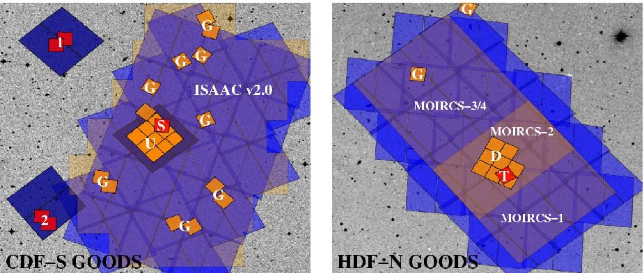
Our primary NICMOS data set includes a somewhat larger number of search fields, some of significant depth, and better optical coverage than was used in our previous search for galaxies (Bouwens & Illingworth 2006: see Figure 1 from the Supplementary Information). The most notable additions are (1) one ultra deep (28.1 AB mag at ) arcmin2 NIC3 pointing within the area of the HUDF (Oesch et al. 2007), (2) ultra deep (28.7 AB mag at ) optical ACS coverage over the second NICMOS parallel to the HUDF (Oesch et al. 2007), and (3) arcmin2 of additional deep (26.7 AB mag at ) NICMOS data within the GOODS area (Riess et al. 2007; H. Teplitz et al. 2008, in preparation).
We have also made improvements to our reductions of the two deep NICMOS fields taken in parallel to the HUDF (Bouwens & Illingworth 2006; Oesch et al. 2007: see Figure 1). Reducing the NICMOS data over these fields is challenging because of the small number of unique dither positions used in the acquisition of the data and the large number of individual frames ( frames in each field). As a result, any systematics present in characterizing the properties of individual pixels on the NIC3 detector propagate directly into the reduced frames, and therefore it becomes necessary to calibrate these properties sufficiently well so that systematics do not have a dramatic effect on the overall noise characteristics. To accomplish this, we generated super median images from a stack of all the NIC3 frames taken over a field, subtracted this median image from each NIC3 frame, and then redrizzled the individual frames together to produce a cleaner reduction. Before generating the super median images, we mask out all sources identified in the image (Szalay et al. 1999) created from our initial reductions of the and band imaging data; sources were masked per NIC3 frame. We elected to use the image for this process to ensure that the same sources were masked in both the and frames. Therefore, the colors of sources were not affected by this “median stacking and subtraction” procedure. To obtain the best possible reduction of the data, we repeated the above procedure several times: using each successive reduction of the data to better mask out the faint sources in the data, median stacking the masked frames, subtracting the medians from the individual frames, and then drizzling the data together to generate a cleaner “final” reduction.
In the dropout searches we performed over the NICMOS data, we only included data which satisfied certain minimal depth requirements in both the optical and near-IR data to avoid the edges of the individual reductions where the number of individual frames contributing to any given pixel was small (i.e., where there might be concerns about some non-Gaussian characteristics in the noise). In our -dropout search, we only included areas where the , , and depths were 27.5 AB mag, 26.8 AB mag, and 26.5 AB mag, respectively, over a 0.6′′-diameter aperture (). We demanded greater depth for our -band imaging data than we did for the -band data given the importance of a robust detection in the -band to making the case for an object being at . For our -dropout search, we only included areas where the , , and -band depths were 27.5 AB mag, 26.8 AB mag, and 26.8 AB mag, respectively, over a 0.6′′-diameter aperture (). We set more stringent requirements on the -band depths for our dropout search because of the greater need to use the -band data to establish the reality of the sources. In total, the area of our search fields were arcmin2 for our -dropout selection and arcmin2 for our -dropout selection.
| 5 Depthbb depths for ACS and NICMOS data given in terms of a -diameter aperture and in terms of a -diameter aperture for the ground-based -band data. In contrast to the detection limits quoted in some of our previous work, here our detection limits have been corrected for the nominal light outside these apertures (assuming a point source). The detection limits without this correction are typically mag fainter. | ||||||
|---|---|---|---|---|---|---|
| Name | Area | RefccReferences: [1] Dickinson 1999, [2] Kajisawa et al. 2006, Ouchi et al. 2007, [3] Thompson et al. 1999, [4] Thompson et al. (2005), [5] Labbé et al. (2006), [6] Oesch et al. 2007, [7] Bouwens & Illingworth (2006), Riess et al. (2007), H. Teplitz et al. (2008, in prep) [8] B. Vandame et al. 2008, in prep; J. Retzlaff et al. 2007, in prep, [9] Mannucci et al. 2007, and [10] Stanway et al. (2008). | ||||
| HDF-North Dickinson | 4.0 | 27.6 | 26.8 | 26.8 | 25.4 | [1,2] |
| HDF-North Thompson | 0.8 | 27.6 | 27.8 | 27.9 | 25.4 | [3,2] |
| HUDF Thompson | 5.8 | 28.8 | 27.4 | 27.2 | 25.8 | [4,5] |
| HUDF Stiavelli | 0.7 | 28.8 | 27.9 | 27.7 | 25.8 | [5,6] |
| HUDF-NICPAR1 | 1.3 | 28.4 | 28.4 | 28.2 | – | [6,7] |
| HUDF-NICPAR2 | 1.3 | 28.4 | 28.4 | 28.2 | – | [6,7] |
| GOODS Parallels | 9.3 | 27.3 | 26.9 | 26.7 | ddThe depth of the near-IR data over the CDF-South varies by mag depending upon the observational conditions in which the ISAAC data were taken. | [7] |
| ISAAC v2.0 | 136 | 27.3 | ddThe depth of the near-IR data over the CDF-South varies by mag depending upon the observational conditions in which the ISAAC data were taken. | ddThe depth of the near-IR data over the CDF-South varies by mag depending upon the observational conditions in which the ISAAC data were taken. | ddThe depth of the near-IR data over the CDF-South varies by mag depending upon the observational conditions in which the ISAAC data were taken. | [8,9,10] |
| MOIRCS GTO-2 | 28 | 27.3 | 25.4 | – | 25.4 | [2] |
| MOIRCS GTO-1,3,4 | 84 | 27.3 | 24.0 | – | 24.2 | [2] |
II.2. ISAAC Search Fields
The deep ( AB mag, AB mag at ), wide-area ( arcmin2) ISAAC data over the CDF-South GOODS field (B. Vandame et al. 2008, in prep; J. Retzlaff et al. 2008, in prep) offer us a superb opportunity to constrain the volume density of very bright star-forming galaxies at . While these data are mag shallower than our NICMOS search data considered above (§2.1), they cover times more area and thus are useful for constraining the volume density of the rarer, more luminous -bright galaxies at . These data are most useful for searching for -band dropouts due to the greater depth of the ISAAC -band data. While Mannucci et al. (2007) used an earlier reduction of these data (v1.5) to search for bright dropouts over the CDF-South GOODS field (see also Stanway et al. 2008), here we repeat this selection with our procedures. In doing so, we will be (1) able to more naturally include the search results over these fields with those obtained from our NICMOS fields and (2) be able to take advantage of the additional ISAAC data that have become available over the CDF-S since the completion of the Mannucci et al. (2007) work. The larger data set covers 10% more area in the and bands and 30% more area in the band. We will not be using these images to constrain the volume density of -dropouts because of the limited depth ( mag at ) of the ISAAC and band data.
We make use of the final (v2.0) reductions of the ISAAC data (B. Vandame et al. 2008, in prep; J. Retzlaff et al. 2008, in prep) for our searches. These reductions include arcmin2 of deep and band coverage and arcmin2 of deep band coverage. Of the area with deep J and Ks coverage, only arcmin2 has deep ACS GOODS coverage. This represents 4% more area than considered in the -dropout search by Mannucci et al. (2007) using the v1.5 ISAAC reductions over the CDF-South GOODS field. The FWHM of the PSF varies from to , with a median value of . The depth of the -band data is appropriately 25.5 AB mag for a detection, while for the and band data, the depth is AB mag. Of course, the actual depth varies by several tenths of a magnitude across the mosaic depending upon the precise exposure time of the ISAAC data and the FWHM of the PSF. As in the previous section, we used the same reductions of the ACS GOODS data as we used in our latest paper on the UV LF at , 5, and 6 (Bouwens et al. 2007).
II.3. MOIRCS Search Fields
We can strengthen our constraints on the prevalence of the bright star-forming galaxies at by taking advantage of the very deep wide-area data taken over the HDF-North GOODS field. While there have been a number of independent attempts to obtain deep near-IR coverage over this field (e.g., the WIRC data over the HDF-North described by Erb et al. 2006), perhaps the best near-IR data set (i.e., deepest, widest area) is from the Subaru MOIRCS imaging observations (Kajisawa et al. 2006; Ouchi et al. 2007). This is due to the significant investment of telescope time ( nights) made by the MOIRCS GTO team in obtaining very deep images during March, April, and May of 2006 (additional observations were made in March and April of 2007 but those are not yet public). There are also 2 nights of high quality band data available from a separate GO proposal. One of the main science goals for these observations has been to search for galaxies (e.g., Ouchi et al. 2007).
The raw images were downloaded from the Subaru-Mitaka-Okayama-Kiso Archive (SMOKA: Baba et al. 2002) and then divided into a number of discrete segments, each segment containing 50 images taken one after another in a given filter. Images from each segment were reduced and combined into a single image using the iraf routines in MCSRED (I. Tanaka et al. 2008, in prep). These reductions were then aligned against the ACS GOODS data and then stacked together to produce two very deep near-IR image mosaics in the and bands. These images were flux calibrated by matching sources with those in the KPNO images of the WFPC2 HDF-North (Dickinson 1998) and in overlap regions between adjacent MOIRCS exposures. Since the MOIRCS GTO team took their observations over 4 distinct pointings, the final reductions cover arcmin2 in total. The final reductions reach a AB magnitude of in the band and 25.4 AB mag in the band over the deepest MOIRCS pointing (GTO-2: arcmin2), while the other three pointings (GTO-1,2,4) are some 1.3 mag shallower. The FWHM of the PSF in our reductions was in the band and in the band. The final -band image mosaic include some 56 hours of data, and the final band image mosaic includes some 64 hours of Subaru data.
III. Sample Construction
III.1. Catalog Construction
Our procedures for generating PSF-matched catalogues and selecting and -dropouts are already well-documented in several previous works (e.g., Bouwens et al. 2003; Bouwens et al. 2005; Bouwens & Illingworth 2006; Bouwens et al. 2007). Nonetheless, we will briefly summarize the different steps in our processing here. All images were first PSF-matched to the NICMOS -band data (or -band data in the case of our dropout searches over the ISAAC or MOIRCS data). We then ran SExtractor (Bertin & Arnouts 1996) in double-image mode to perform the object detection and photometry. We generated the detection image by taking the square root of image (Szalay et al. 1999) constructed from the and band images for our -dropout selection and from the band image for our -dropout selection. Colors were measured in a small-scalable aperture using Kron-style (1980) photometry, where the Kron factor was 1.2. These fluxes were then corrected up to total magnitudes using the light within a larger Kron (1980) aperture (adopting a Kron factor of 2.5). These latter corrections were made from the square root of the image to improve the S/N. Figure 5 of Coe et al. (2006) provides a graphical description of a similar multi-stage procedure for measuring colors and total magnitudes. Aperture radii used for total magnitude measurements ranged from arcsec. An additional mag correction was made to account for the light outside of these apertures and on the wings of the PSF (e.g., Thompson et al. 1998).
III.2. Selection Criteria
Our selection criterion for our -dropout search was as shown in Figure 2, where represents the logical AND operation. This criterion is identical to the “less conservative” -dropout selection criterion of Bouwens & Illingworth (2006). We opted to use this criterion rather the more stringent “conservative” criterion from that same work for two reasons. First, we realized that our “conservative” criterion may have been more stringent than necessary to reject contaminants like T-dwarfs (low mass stars) from our samples. These contaminants can (in most cases) be rejected by a procedure we will describe below. Second, by adopting a “less conservative” selection criteria, the effective selection volumes will be larger and therefore less sensitive to small inaccuracies in the assumed model galaxy population.
For regions of the two GOODS fields with ISAAC/MOIRCS coverage, our -dropout criterion was . This selection criterion is very similar to the criterion used over our NICMOS fields. For the typical star-forming galaxy at (with a -continuum slope of ) this criterion selects galaxies to a slightly lower-redshift limit than our NICMOS -dropout criterion (where ).
The criterion for our -dropout search was . We elected to use a less restrictive color criterion than the criterion used in our previous -dropout search (Bouwens et al. 2005) because of the availability of deep optical data over almost all of our previous search fields to eliminate low redshift interlopers. Previously ultra deep optical data were not available over the NICMOS parallels to the HUDF, and so we accordingly decided to select dropouts using a more stringent color cut.
In computing the and colors that we used for our and dropout selections, we set the - and -band fluxes to their upper limits in the case of non-detections. This was to minimize the extent to which faint sources in our search fields would scatter into our dropout samples.
Sources in our and -dropout selections were also required to be detected at the level in the band within a 0.6′′ diameter aperture (to eliminate spurious sources) and undetected () in the available , , or band imaging. Sources which were detected at the level in more than one of the ACS , , and bands were also rejected as low-redshift interlopers. Possible contamination by low mass stars (which are a concern for our -dropout selection) are identified by looking for sources which showed faint detections () in the -band in a -diameter aperture and whose -band profile appeared to be consistent with a point source (i.e., the SExtractor stellarity parameter ).
All candidate dropouts were inspected in the available IRAC and MIPS coverage over the two GOODS fields (Dickinson & GOODS team 2004) to ensure that none had particularly red mag or mag colors. With the exception of the two sources which satisfy our -dropout criterion (03:32:41.22, :44:00.8 and 03:32:32.45, :42:21.5), none of the sources which satisfied our other criteria were found to have such red infrared colors (or showed significant detections at , , or ).
The two particularly red dropouts (with magnitudes of and , respectively) have colors of mag and are even detected at in the available MIPS imaging over the GOODS fields (meaning that their apparent magnitudes at m are mag). Since we do not expect galaxies at to be so bright at and otherwise so highly reddened (but see also discussion in Wiklind et al. 2007), we have excluded these sources as candidate galaxies.


III.3. Selection Results
Application of our selection criteria across all the fields given in Table 1 yielded 8 credible -dropout candidates, but no credible -dropout candidates. All 8 of our -dropout candidates were found in our NICMOS search fields. The properties of each of the 8 -dropout candidates are given in Table 2. Figure 3 provides a postage stamp montage of the 8 candidates. We also included one candidate we identified in a separate search around massive lensing clusters (Bradley et al. 2008; Bouwens et al. 2008). Five of the eight candidates were given in our two previously published -dropout searches (Bouwens et al. 2004c; Bouwens & Illingworth 2006). Three of these candidates are new. Two of the three new candidates (UDF-3244-4727 and NICPAR1-3303-4111) were just below the flux thresholds used in our previous searches, but meet these thresholds now as a result of modest improvements in the S/N and overall quality of our NICMOS reductions. The third candidate (NICPAR2-3308-5229) was found over the second NICMOS parallel to the HUDF and could be identified as a result of the much deeper optical (ACS) data now available over these fields to set strong constraints on the colors. Our sample also includes one -dropout (UDF-380-1125) which, while appearing in the our initial -dropout selection over the HUDF (Bouwens et al. 2004c), did not appear in our more recent Bouwens & Illingworth (2006) selection because of the more conservative S/N threshold used in that work.
| Object ID | R.A. | Dec | RefaaReferences: [1] Bouwens et al. (2004c), [2] Bouwens & Illingworth (2006), [3] Yan & Windhorst (2004), [4] Coe et al. (2006), [5] Labbé et al. (2006), [6] Bradley et al. (2008) | ||||
|---|---|---|---|---|---|---|---|
| HDFN-3654-1216 | 12:36:54.12 | 62:12:16.2 | [2] | ||||
| UDF-640-1417 | 03:32:42.56 | 27:46:56.6 | [1,2,3,4,5] | ||||
| NICPAR2-3308-5229bbThere appears to be some flux in the band very close to the position of this source (). If this flux is associated with this source and not a chance superposition, it would rule out this source being a galaxy. The existence of a small amount of flux in the band would be somewhat unexpected given that there is no detectable flux in the and bands and the fact that these exposures reach similar flux limits. On balance, we consider this to be a likely candidate. | 03:33:08.29 | 27:52:29.2 | ccUpper and lower limits on the measured colors are the limits. | — | — | ||
| CDFS-3225-4627 | 03:32:25.22 | 27:46:26.7 | ccUpper and lower limits on the measured colors are the limits. | [2] | |||
| UDF-983-964 | 03:32:38.80 | 27:47:07.2 | ccUpper and lower limits on the measured colors are the limits. | [1,2,4,5] | |||
| UDF-387-1125 | 03:32:42.56 | 27:47:31.4 | ccUpper and lower limits on the measured colors are the limits. | [1,5] | |||
| UDF-3244-4727 | 03:32:44.02 | 27:47:27.3 | ccUpper and lower limits on the measured colors are the limits. | ccUpper and lower limits on the measured colors are the limits. | — | ||
| NICPAR1-3303-4111ddBecause this source (detected at ) was found over the NICMOS parallels to the HUDF and the noise properties of these data may exhibit significant non-Gaussian characteristics due to the small number of unique dither positions (see §2.1), we took special care in assessing the reality of this source. We considered all the available NICMOS data at 4 highly distinct dither positions (separated by each) and in both the and -band data separately. The candidate was evident at significance in 7 of the 8 of the stacks, consistent with what we might expect if the candidate were a real source. This source is also present in an independent reduction of these data (Oesch et al. 2008). | 03:33:03.81 | 27:41:12.1 | ccUpper and lower limits on the measured colors are the limits. | — | — | ||
| —————————————————————————— | |||||||
| A1689-zD1eeThis source was identified in a separate search for -dropouts behind massive galaxy clusters (Bradley et al. 2008; Bouwens et al. 2008) and is not used here for deriving the LF at . This source is substantially magnified by gravitational lensing from Abell 1689 (). Its delensed -band magnitude is AB mag (Bradley et al. 2008). | 13:11:29.73 | 01:19:20.9 | ccUpper and lower limits on the measured colors are the limits. | — | [6] | ||
There were two sources in our catalogues which while satisfying our -dropout color criteria did not make it into our -dropout selection because of their compactness in the -band, which strongly suggested they were T dwarfs (03:32:25.10, :46:35.6 and 12:37:34.26, 62:18:31.4). These sources had previously been identified as possible T dwarfs in a number of other studies (Bouwens & Illingworth 2006; Mannucci et al. 2007; Eyles et al. 2007). There were also 28 sources in our selection that while satisfying our -dropout color criteria showed significant detections () in the , , or bands and thus were excluded from our -dropout selection. One possible -dropout candidate over the near-IR ISAAC data was found at 03:32:24.74, :55:15.8. This source seemed to be a plausible candidate, with an apparent detection in the band, an apparent -band magnitude of 24.80.2 AB mag, and no detection () in any of the optical imaging data. However, since this source is undetected ( [ limit] in a -diameter aperture) in even deeper NICMOS -band data over this field, it seems highly likely that this source is spurious (or perhaps a SNe: see §3.4).
In Appendix D, we discuss several sources which appeared in previous dropout samples of ours but do not appear in the current selections.
III.4. Contamination
We give particular attention to contamination, since it can be a significant issue in searches for very faint, high-redshift galaxies. This discussion is only relevant for our -dropout selection since our -dropout selection contains no credible candidates. There are four types of contaminants that are of particular concern: (i) T-dwarfs, (ii) supernovae, (iii) lower-redshift galaxies which may move into our -dropout selection through photometric scatter, and (iv) spurious sources.
Possible Contamination from T dwarfs: T dwarfs are low-mass brown dwarfs, which while most well known and studied in the solar neighborhood (e.g., Knapp et al. 2004; Burgasser et al. 2006), are sometimes observed at great distances and therefore can be quite faint (i.e., : Ryan et al. 2005; Bouwens & Illingworth 2006). Since T dwarfs occupy a position in color-color space very similar to that of high-redshift galaxies (Figure 2), they can therefore be difficult to distinguish from star-forming galaxies at on the basis their photometry alone. This leaves us with the size or morphology of these sources as essentially our only means of distinguishing these sources from galaxies. This enterprise is made more difficult because the T dwarfs are brightest in exactly the same data (near-IR) where the resolution is the poorest. Fortunately, the available ACS data have sufficient depth and resolution that any T dwarfs in our data should show up as point sources. This follows from the fact that all candidate dropouts in our sample are detected at , T dwarfs have colors of mag, and the ACS -band data are at least mag deeper in a -diameter aperture (ACS resolution) than our near-IR data is in a -diameter aperture (near-IR resolution: see Table 1).11 1 The depths of the ACS data in a -diameter aperture is mag deeper than that given in Table 1 (for a -diameter aperture). Since none of the -dropouts in our selection show -pointlike detections in the available -band coverage, this suggests that these sources are not T dwarfs.
Possible Contamination from Supernovae: Since the NICMOS data were largely taken at quite different times than the ACS data, it is quite possible that highly time-variable sources like supernovae could show up as dropouts in our selections. To estimate the approximate frequency at which we might expect such sources to show up in our searches, we adopted the GOODS supernova searches (Riess et al. 2004; Strolger et al. 2004) as a baseline. In their searches, they identified 42 supernovae in 8 independent searches over one of the two arcmin2 GOODS fields (15 ACS WFC pointings), or supernovae per arcmin2 ACS WFC field per day period. Of these supernovae, only % of the high-redshift supernovae identified by Riess et al. (2004) and Strolger et al. (2004) appear to be well enough separated from their host galaxies to be identified as a separate source. Having calculated the approximate rate at which supernovae appear at random in deep fields, all that remains is to calculate the time period over which we might expect these supernovae to show up as possible sources in our search. While theoretically we might expect high-redshift SNe to be bright enough to show up in our survey data for days (if we take the typical light curves found in e.g., Strolger et al. 2004), all -dropouts in our sample are within mag of the flux limit of each survey field. Typical SNe (at ) would not remain at these magnitudes for more than days, so the incidence of SNe in our probe should be for data taken at different epochs. Multiplying this by the arcmin2 of NICMOS data in our search taken at significantly different times than the ACS data (the HUDF NICMOS data were taken at a similar time to the ACS HUDF data), we would expect that only 0.2 supernovae should contaminate our high redshift selections. While this number is just 3% of the 8 sources in our -dropout selection and therefore likely of minimal importance for the present LF determinations, it does indicate that contamination of high-redshift selections by supernovae is a real possibility. This may be a particularly important concern in searches for bright galaxies due to the inherent rarity of those sources.
Possible Contamination Through Photometric Scatter: One possible source of contamination are low redshift sources scattering into our color selection simply because of noise. To assess the importance of this effect, we ran a number of Monte-Carlo simulations where we started with a low-redshift galaxy population and then added noise to the fluxes in the individual bands to see how many of the sources would satisfy our -dropout selection. Clearly, the most critical aspect of these simulations is ensuring that the properties of the input galaxy population (to which noise is added) are accurate. We set up the input population as follows: (1) The input magnitudes and photometric errors are modelled using the actual distribution of magnitudes and errors found in the data (to make our estimates as model independent as possible and because essentially all faint sources in our fields will be at ) and (2) The colors (i.e., optical- and ) of the input population are assumed to be distributed in the same way as is observed for galaxies in the range in the HUDF (ACS+NICMOS coverage). We used galaxies in this magnitude range because of their higher S/N colors and because the multivariate color distribution is similar (albeit slightly redder) to galaxies at -band magnitudes AB mag. This magnitude range also does not include any sources which are candidate galaxies (at least in the HUDF).
Based upon the described input population, we ran 10 separate photometric scattering experiments for each search field. We estimated that there would be 0.0, 0.3, 0.2, and 0.3 low-redshift contaminants, respectively, for our -dropout selections over the HUDF, NICPAR, HDFN, and GOODS parallel fields. In total, contaminants are expected from all our fields. We note that the approach taken here to estimate contamination from photometric scatter is analogous to the one described in Bouwens et al. (2004c) or Appendix D.4.2 of Bouwens et al. (2006).
Possible Contamination from Spurious Sources: Finally, to estimate the number of contaminants from spurious sources, we repeated our selection procedure on the negative images (e.g., Dickinson et al. 2004; Yan & Windhorst 2004; Bouwens et al. 2007) and found no sources that satisfied our selection. This suggests that the spurious fraction is negligible. We note that we would not expect contamination from spurious sources to be a problem since essentially all of the sources in our sample are detected at in both the and bands. The only notable exceptions to this are for the two sources in our sample, UDF-387-1125 and UDF-3244-4727, where -band detections are still only at the level. However, in both cases, we are attempting to improve the detection significance (as well as the S/N of the and colors) by obtaining an additional 9-12 orbits of -band data on both sources (likely improving their detection significance to the level).
In summary, the overall level of contamination should be fairly low in general. We would expect galaxy to enter our sample from photometric scatter, SNe contaminants to enter our sample, and there to be no contamination from T dwarfs or spurious sources. Overall, this suggests an overall contamination level of %.
IV. Determinations of the UV LF at
We now utilize our search results to determine the rest-frame LF at . We will consider both LFs using both stepwise and Schechter parametrizations. The advantage of the stepwise determinations is that they give a more model-independent measure of the constraints we have on the LF, while the Schechter determinations are more amenable to direct interpretation and comparison with other determinations in the literature.
As in other methodologies for determining the LF, we maximize the probability with which our model LFs are able to reproduce our search results. Since we do not know the precise redshifts for our sources, our goal will simply be to reproduce the surface density of -dropout candidates in each of our search fields as a function of apparent magnitude. This is similar to the modelling we performed in our previous paper on the LFs at , , and (Bouwens et al. 2007), where we attempted to reproduce the surface density of , , and dropouts in deep ACS fields.
To maximize the likelihood with which our model LFs reproduce our search results, we need to be able to compute the expected surface density of dropouts as a function of magnitude. We use a similar formalism to the one we used in our previous paper on the LFs at :
| (1) |
where is the surface density of galaxies in some search field with magnitude , is the volume density of galaxies with absolute magnitude , and is the effective selection volume for which galaxies with absolute magnitude will both satisfy our dropout selection criteria and be observed to have an apparent magnitude . The width of the magnitude bins in , , and will depend upon the LF parameterization we consider (stepwise vs. Schechter).
We computed the effective volumes for our and dropout selections by artificially redshifting -dropouts from the HUDF across the selection windows of our higher redshift samples, adding the sources to the real data, and then repeating our selection procedure. We used our well-tested cloning software (Bouwens et al. 1998a,b; Bouwens et al. 2003) to handle the artificial redshifting of sources from to . The size of the sources were scaled as (independent of luminosity) to match the size trends observed for star-forming galaxies at (Bouwens et al. 2006; see also Ferguson et al. 2004 and Bouwens et al. 2004c). The redshifted (“cloned”) sources were smoothed so that their effective PSFs matched that seen in the data. The mean -continuum slope was set to to agree with that observed in star-forming galaxies at (Stanway et al. 2005; Bouwens et al. 2006; Yan et al. 2005) while the dispersion in was set to 0.5, which is similar to what is found at (e.g., Bouwens et al. 2007; R.J. Bouwens et al. 2008, in prep). Instead of using simple power laws to represent model SEDs of given continuum slope , we elected to use -yr continuous star-formation models (Bruzual & Charlot 2003) where the dust extinction (Calzetti et al. 1994) is varied to reproduce the model slopes. This should provide for a slightly more realistic representation of the SEDs of star-forming galaxies at than can be obtained from simple power law spectra.
To evaluate the likelihood with which the surface densities computed above would reproduce that found in the observations, we assumed simple Poissonian statistics and compared the observed and expected numbers bin by bin. In detail, our expression for the likelihood is
| (2) |
where is the observed number of sources in search field and magnitude interval , where is the expected number of sources in search field and magnitude interval , and where is the product symbol. We elected to use the above procedure instead of a more conventional procedure like STY79 (Sandage, Tammann, & Yahil 1979) or SWML (Efstathiou et al. 1988: which determine the shape of the LF independent of the normalization) to take advantage of our search constraints on the volume density of bright galaxies from our wide-area ground-based data. Maximum likelihood procedures (like SWML or STY79) do not take advantage of these null search results – simply because there are no sources to use for estimating the shape of the LF. While the maximum likelihood fit results from Eq. 2 will be affected by large-scale structure variations across our search fields, we will compute the uncertainties which result from these variations in §4.1, §4.2, and Appendix A and include them in our overall error budget.
In determining the rest-frame UV LF at and from our and dropout selections, we will adopt and , respectively, as the fiducial redshifts for these selections and the derived LFs. In §4.2, we will justify the use of these mean redshifts using the effective volume simulations just described (see also Bouwens et al. 2004; Bouwens et al. 2005; Bouwens & Illingworth 2006).
IV.1. Stepwise Determinations
We begin with a determination of the LF at and in stepwise form. The advantage of stepwise parametrizations is that they allow us to determine the overall prevalence of galaxies in a way that is very model independent and just a simple function of luminosity. The width of the bins in the LF are 0.8 mag and was chosen as a compromise between the need to have a few galaxies per bin and the desire to retain a reasonable resolution in luminosity for our derived LFs. We use a similar bin size for the stepwise upper limits on our -dropout LF in order to make these limits more easily interpretable. The stepwise LF is then derived using Eq. 1. The results are presented in Table 3.
Perhaps the largest uncertainties in these LF determinations arise from small number statistics (Poissonian errors). However, in addition to the simple number statistics, there are also sizeable uncertainties that come from large-scale structure variations as well as our effective volume estimates. Let us first consider the uncertainties coming from large-scale structure variations. Adopting a pencil beam geometry, redshift selection window with width , search area of 100 arcmin2, and bias of 7 (which is appropriate for sources with volume densities of Mpc-3: e.g., Mo & White 1996; Somerville et al. 2004; Trenti & Stiavelli 2008), we estimate a RMS uncertainty of 30% in the ’s due to field-to-field variations (see also estimates in Bouwens & Illingworth 2006). At , these uncertainties are % assuming a redshift selection window with width (see Bouwens et al. 2005).
Uncertainties in our effective volume estimates derive primarily from our imperfect knowledge of the size (or surface brightness) distribution of star-forming galaxies at .22 2 Uncertainties in the UV color distribution also contribute to the overall error budget for our effective volume estimates, but they are smaller in general (e.g., see §5.2). Fortunately, the mean size of star-forming galaxies at show a good correlation with redshift (i.e., mean half-light radius for fixed luminosity: Bouwens et al. 2006) and we can make a reasonable estimate for what the size (surface brightness) distribution of galaxies is at . Nonetheless, this distribution is at least as uncertain as the error on the size-redshift scaling. Propagating the error on this scaling into the size distributions assumed in our effective volume estimates, we estimate an RMS uncertainty of 17% in the selection volume at and 15% at due to the uncertainties in the size (surface brightness) distribution. Together the size and large-scale structure uncertainties add an uncertainty of 34% and 25% RMS to each bin of the rest-frame UV LF at and , respectively. These uncertainties have been added in quadrature with those deriving from the small number statistics. They are given in Table 3.
| bbThe effective rest-frame wavelength is for our -dropout selection and for our -dropout selection. | (Mpc-3 mag-1) |
|---|---|
| -dropouts () | |
| aaUpper limits here are (68% confidence). | |
| -dropouts () | |
| aaUpper limits here are (68% confidence). | |
| aaUpper limits here are (68% confidence). | |
| aaUpper limits here are (68% confidence). | |
| aaUpper limits here are (68% confidence). | |
These LFs are also presented in Figure 4 with the magenta points for our LF and black downward arrows for the constraints on the LF. A comparison with previous determinations at , , and from Bouwens et al. (2007) is also included on this figure for context. Though the error bars for individual points in the LF at are still quite sizeable, there is strong evidence that the UV LF at is different from the UV LF at (99% confidence) and thus there is evolution from to . We determined this confidence level by finding the value of and which minimizes the total evaluated for our and dropout LFs and then looking at the probability of obtaining the resultant reduced- purely by chance. This conclusion was already drawn by Bouwens & Illingworth (2006) on the basis of a smaller but very similar selection of galaxies.


IV.2. Schechter Determinations
We will now attempt to express the results of our search for galaxies using a Schechter parameterization. The Schechter parametrization is convenient since it is much more amenable to interpretation than stepwise LFs are. Of course, it is not at all clear from the stepwise LFs derived in §4.1 (particularly given the sizeable observational uncertainties) that the LF at is well described by a Schechter function (see discussion in §5.5).
As with our stepwise determinations, we will calculate the expected surface density of dropouts given a model LF by using Eq. 1 and expressing the Schechter function in stepwise form. For convenience, we have decided to bin the surface density of galaxies in magnitude intervals of width 0.1 mag. Use of substantially finer bins does not have a noticeable effect on the results. Because of the size of current samples and limited luminosities ( AB mag) to which we can probe, we cannot hope to obtain very strong constraints on the faint-end slope of the LF at and therefore it makes sense for us to fix it to some fiducial value. We will adopt , which is the faint-end slope of the LF at determined by Bouwens et al. (2007) using the HUDF and a large number of deep ACS fields. Later we will investigate the sensitivity of our results to the value we assume for the faint-end slope.
| Dropout | ||||
|---|---|---|---|---|
| Sample | aaValues of are at for the Bouwens et al. (2007) and -dropout LFs, at for the Bouwens et al. (2007) -dropout LF, at for our -dropout LF, and at for our constraints on the -dropout LF. Since galaxies are blue (: Stanway et al. 2005; B06), we expect the value of at to be very similar ( mag) at to its value at . Similarly, we expect the value of at and to be fairly similar at to the values determined at and , respectively. | Mpc-3) | ||
| 7.3 | bbFixed in our fits (§4.2) | |||
| 9.0 | ccLower limits here are (68% confidence). | bbFixed in our fits (§4.2) | bbFixed in our fits (§4.2) | |
| —————————————————————– | ||||
| 3.8 | ||||
| 5.0 | ||||
| 5.9 | ||||

Our best-fit Schechter parameters at for our -dropout selection are mag and Mpc-3 for a fixed faint-end slope . The 68% and 95% likelihood contours for these parameters are given in Figure 5 and compared with our previous determinations from our , , and -dropout selections at , , and , respectively (Bouwens et al. 2007). The best-fit values are also given in Table 4. Large-scale structure uncertainties resulting from field-to-field variations were estimated using Monte-Carlo simulations (Appendix A) and incorporated into the uncertainties quoted above. While the best-fit value for is very similar to that found at for the Bouwens et al. (2007) -dropout selections, the best-fit value for is mag fainter than the value of (= mag) found at by Bouwens et al. (2007) and mag fainter than the value of ( mag) found at by Bouwens et al. (2007). This suggests that the brightening we observe in from to (Bouwens et al. 2006; Bouwens et al. 2007) is also seen from . Of course, we must admit that we are somewhat surprised that our best-fit Schechter parameters are in such excellent agreement with an extrapolation of lower redshift trends! It would suggest that our -dropout sample may largely be made up of star-forming galaxies at as we have argued in §3.3 and §3.4 (i.e., the number of low-redshift interlopers is small) and that the effective volumes we have estimated for this sample are reasonably accurate (see also discussion in Appendix B).
| Dropout | ||||
|---|---|---|---|---|
| Sample | aaSee remarks in Table 4. | Mpc-3) | ||
| 7.3 | bbFixed in our fits (§4.2) | |||
| 7.3 | bbFixed in our fits (§4.2) | |||
| 7.3 | bbFixed in our fits (§4.2) | |||
| 9.0 | ccLower limits here are (68% confidence). | bbFixed in our fits (§4.2) | bbFixed in our fits (§4.2) | |
| 9.0 | ccLower limits here are (68% confidence). | bbFixed in our fits (§4.2) | bbFixed in our fits (§4.2) | |
| 9.0 | ccLower limits here are (68% confidence). | bbFixed in our fits (§4.2) | bbFixed in our fits (§4.2) | |
| 9.0 | bbFixed in our fits (§4.2) | ccLower limits here are (68% confidence). | bbFixed in our fits (§4.2) | |
| 9.0 | bbFixed in our fits (§4.2) | ccLower limits here are (68% confidence). | bbFixed in our fits (§4.2) | |
| 9.0 | bbFixed in our fits (§4.2) | ccLower limits here are (68% confidence). | bbFixed in our fits (§4.2) |
Given the small size of current -dropout samples, it may seem surprising that we are able to obtain any constraint at all on the shape on the LF at . Fortunately, the large luminosity range over which we have constraints on the surface density of dropouts (i.e., from 25 AB mag to 28 AB mag) largely makes up for what we lack in statistics. These constraints can be helpful, even brightward of 26.0 AB mag where our -dropout sample contains no sources, because of the large search areas we consider (248 arcmin2). To illustrate how our search results help us constrain the overall shape of the LF, we show in Figure 6 the predicted counts for each of our search fields from our best-fit LF (i.e., mag, Mpc-3) in red and compare it against the best-fit model where shows no evolution from (green lines: , Mpc-3). The observed surface densities of dropouts are shown with the solid histogram. As is apparent from this figure, the model with the bright value of predicts too many bright sources (e.g., ISAAC/MOIRCS panel) and too few faint sources (e.g., HUDF panel), whereas the model with a fainter value of provides a better match to the observations. The significance of this result, however, is clearly only modest () at present, given the limited statistics. Better statistics would also be helpful for verifying that our treatment of the selection effects in each search field is reasonably accurate.
For our -dropout selection, we cannot derive a set of best-fit Schechter parameters due to the lack of any dropout candidates in our sample. Nonetheless, it does make sense for us to set constraints on and assuming no evolution in the other Schechter parameters from . For example, supposing there is no evolution in (i.e., ), we can set a upper limit of Mpc-3 ( lower than at ) on . Similarly, assuming there is no evolution in (i.e., Mpc-3), we can set a lower limit of AB mag (1.4 mag fainter than at ) on . The joint constraints on the value of and are shown in Figure 5 with the black lines indicating the 68% and 95% confidence limits.

In constraining the Schechter parameters at and from our and -dropout searches, we assumed that the faint-end slope was equal to the same value we had previously determined at , i.e., . To see how these constraints might depend upon the assumed faint-end slope , we repeated the determinations assuming a faint-end slope of and . The results are presented in Table 5, and it is clear that the derived values for and only show a mild dependence on the assumed faint-end slope , particularly when compared to the uncertainties on these two parameters from other error sources (e.g., from small number statistics). We can therefore essentially ignore the effect of the uncertain faint-end slope on our quoted constraints for both and .
To put the LF fit results and dropout selections in context, it seems helpful to use our best-fit LFs to calculate an expected redshift distribution for our and dropout selections. We can take advantage of the same simulations described at the beginning of §4 to calculate these redshift distributions. For concreteness, and are assumed for the LF at for our -dropout selection (using the extrapolations from §5.3). The redshift distributions are presented in Figure 7. The mean redshifts expected for our z-dropout and J-dropout selections are 7.3 and 9.0, respectively. The mean redshifts estimated for both selections are smaller than what we had considered in previous works (e.g., Bouwens et al. 2004c; Bouwens et al. 2005; Bouwens & Illingworth 2006) because of our adoption of a slightly more inclusive dropout criterion in this work. Note that including the likely evolution across the redshift range of these selections would likely lower the mean redshifts even more (Muñoz & Loeb 2008).


| SFR density | ||||
|---|---|---|---|---|
| (ergs s-1 | ( Mpc-3 yr-1) | |||
| Sample | Hz-1 Mpc-3) | Uncorrected | CorrectedbbThe adopted dust-extinction corrections are 0.4 mag, 0.6 mag, and 1.1 mag at , , and , respectively. Our use of an evolving dust correction from to is motivated by the apparent evolution in -continuum slope over this redshift range (e.g., Stanway et al. 2005; Bouwens et al. 2006) and the correlation of -continuum slope with dust extinction (e.g., Meurer et al. 1999; Reddy et al. 2006). | |
| 7.3 | 25.320.21 | |||
| 9.0 | ccUpper limits here are (68% confidence). | ccUpper limits here are (68% confidence). | ccUpper limits here are (68% confidence). | |
| —————————————————————– | ||||
| 3.8 | 26.180.05 | 0.05 | ||
| 5.0 | 25.850.06 | 0.06 | ||
| 5.9 | 25.720.08 | 0.08 | ||
IV.3. Luminosity / SFR density
We can use the present LF results to refine our constraints of the rest-frame luminosity densities at . Previously, we set constraints on these quantities based upon a sample of four -dropout candidates found over the GOODS fields (Bouwens & Illingworth 2006) and a sample of three possible -dropout candidates over the deep NICMOS parallels to the HUDF (Bouwens et al. 2005).
Here we are able to make modest but significant improvements in our measurement of the luminosity density at . We make these estimates based upon our best-fit LFs at and . We shall consider integrations to a limiting luminosity of 0.2 because this corresponds to the approximate flux limit for our and -dropout searches (i.e., ). We present these luminosity densities in Figure 8 and Table 6. As is conventional, we also present the equivalent star formation rate on this same figure using the Madau et al. (1998) and adopting a Salpeter IMF. To show how this situation changes when a plausible account of dust is included, we plot the equivalent dust-corrected and uncorrected SFR densities in Figure 9. We employ the dust corrections adopted by Bouwens et al. (2007), which are 1.4 mag, 1.1 mag, 0.6 mag, and 0.4 mag at , , , and , respectively. Our use of an evolving dust correction from to is motivated by the apparent evolution in the -continuum slope over this redshift range (e.g., Stanway et al. 2005; Bouwens et al. 2006) and the correlation of -continuum slope with dust extinction (e.g., Meurer et al. 1999; Reddy et al. 2006).
V. Discussion
V.1. How does the volume density of -bright galaxies evolve?
Over the past few years, there has been some controversy regarding how the UV LF evolves at high redshift. While some studies have argued that the evolution primarily occurs at the bright end (i.e., Dickinson et al. 2004; Shimasaku et al. 2005; Ouchi et al. 2004a; Bouwens et al. 2006; Yoshida et al. 2006; Bouwens et al. 2007), there have been other efforts which have argued that the evolution occurs primarily at the faint end (i.e., Iwata et al. 2003; Sawicki & Thompson 2006; Iwata et al. 2007). In this work, we found additional evidence to support the fact that the most rapid evolution occurs at the bright end of the LF and that this evolution can be approximately described by a change in the characteristic luminosity of the UV LF.
A significant part of the debate regarding the form the evolution of the LF takes at high redshift is centered on what happens at the bright end of the LF (i.e., ). Does it evolve or not? Iwata et al. (2007) and Sawicki & Thompson (2006) argue that there is little evidence for substantial evolution from to from their work. However, a quick analysis of results in the literature indicate that such evolution is certainly very strong, particularly if the baseline is extended out to even higher redshifts (). At , for example, the bright end of the LF (i.e., ) has been reported to be deficient by factors of relative to (Stanway et al. 2003, 2004; Shimasaku et al. 2005; Bouwens et al. 2006). At , this deficit is even larger, as we can see by comparing the number of bright galaxies (i.e., ) in our dropout selections with that expected from (Bouwens et al. 2007) assuming no-evolution. The comparisons are presented in Table 7. At , the volume density of bright () galaxies appears to be smaller than at (see also Bouwens & Illingworth 2006; Mannucci et al. 2007; Stanway et al. 2008), and at , the volume density of bright galaxies is at least 16 smaller (68% confidence).
| Number | Evolutionary | ||
|---|---|---|---|
| Sample | Observed | PredictionaaExtrapolations assume no evolution in the LF from (Bouwens et al. 2007) and were calculated using Eq. 1. The sizes and colors of -bright galaxies at assumed for these estimates are the same as those given in Appendix B. | FactorbbRatio of volume density of galaxies at (Bouwens et al. 2007) in some luminosity range to that in our higher redshift dropout samples. |
| Bright () | |||
| -dropout | 2 | 35.9 | |
| -dropout | 0 | 17.9 | ccLower limits here are (68% confidence). |
| Faint () | |||
| -dropout | 6 | 24.7 | |
| -dropout | 0 | 8.0 | ccLower limits here are (68% confidence). |
The only analysis to find mild evolution in the volume density of bright galaxies from to is that of Richard et al. (2006) and involves a search for galaxies behind lensing clusters. However, as we argue in Appendix C, it seems likely that a substantial fraction of the -bright galaxies in the Richard et al. (2006) selection are spurious and therefore the bright end of their LFs is much too high. The evidence for this is rather striking: not only are none of the candidates in the Richard et al. (2006) selection detected () in significantly deeper (1-2 mag) NICMOS+IRAC data (11 of their candidates), but also their reported prevalence is higher than what we measure in searches for similar candidates behind lensing clusters (Bouwens et al. 2008; see also Appendix C).
Considering the substantial evolution found from to in the volume density of bright galaxies, it is certainly relevant to note that all three previous studies (i.e., Iwata et al. 2003; Sawicki & Thompson 2006; Iwata et al. 2007) which argued for less evolution at the bright end of the LF than at the faint end did not extend to redshifts much higher than 4. In fact, the very mild evolution (or no-evolution) at the bright end of LF claimed by the above studies seems to be highly consistent with other analyses in this redshift range (e.g., Steidel et al. 1999; Reddy et al. 2007) which in general find very little evolution from to . Even for the Iwata et al. (2007) LF at (which is fairly similar to the LFs at at bright luminosities), one may not expect much evolution at the bright end. After all, the mean redshift of their bright selection is , which is not much higher than .33 3 The mean redshift for bright galaxies in the Iwata et al. (2007) selection is likely to be somewhat lower in redshift than for the fainter ones. This is because (1) the Iwata et al. (2007) selection window extends to somewhat lower redshift for the redder star-forming galaxy population than it does for the bluer star-forming galaxy population and (2) brighter star-forming galaxies at are observed to have much redder UV colors in general than the fainter star-forming galaxies at these redshifts (e.g., Meurer et al. 1999; Iwata et al. 2007; R.J. Bouwens et al. 2008, in prep). As a result, the mean redshift for bright galaxies in the Iwata et al. (2007) selection will be lower than for the faint galaxies, and therefore the bright end of the Iwata et al. (2007) LF should show less evolution than the faint end.
In summary, it would appear that the most reasonable conclusions to draw from these studies are that the bright end of the LF shows substantial evolution at very high redshifts () and then mild evolution at somewhat later times (i.e., from to ).
V.2. Completeness of current samples in -continuum slope
The selection criteria we use to select star-forming galaxies at (and at ) differ somewhat in the efficiency with which they select galaxies that have red -continuum slopes , i.e., .44 4 For our -dropout selection, for example, we would only be moderately effective at selecting galaxies with -continuum slopes redder than (Figure 2). For our -dropout selection, on the other hand, there is no limit on how red a star-forming galaxy can be in terms of its -continuum slope, except as set by our restrictions on the IRAC and MIPS colors of sources (i.e., , : see §3.2) which require . For the Bouwens et al. (2007) -dropout, -dropout, and -dropout selections, we are only effective in selecting star-forming galaxies, if their -continuum slopes are bluer than (see Figure 8 of Bouwens et al. 2007). This would potentially have an effect on our determinations of the LFs if such red star-forming galaxies existed in large numbers. Fortunately, for these dropout selections, it appears that they do not. At , for example, both Lyman-break and Balmer-break selections almost entirely consist of galaxies with ’s bluer than (§4.1 and Figure 8 of Bouwens et al. 2007; Brammer & van Dokkum 2007). At , the galaxy population appears to be bluer yet, with mean ’s of (e.g., Stanway et al. 2005; Bouwens et al. 2006; Yan et al. 2005; Lehnert & Bremer 2003; Hathi et al. 2008), and there is little evidence from the present selections that the galaxy population is any less blue at . Indeed, the observed colors are consistent with a star-forming population with little dust and years of constant star formation (where : see Figure 12).
| Dropout | Mean | ||||
|---|---|---|---|---|---|
| Sample | bbSee remarks in Table 4. | Mpc-3) | |||
| 7.3 | |||||
| 7.3 | ddBoth bluer and redder -continuum slopes can result in slightly lower estimated selection volumes for star-forming galaxies at . | ||||
| 7.3 | ddBoth bluer and redder -continuum slopes can result in slightly lower estimated selection volumes for star-forming galaxies at . | ||||
| 9.0 | ccLower limits here are (68% confidence). | eeFixed in our fits. | |||
| 9.0 | ccLower limits here are (68% confidence). | eeFixed in our fits. | |||
| 9.0 | ccLower limits here are (68% confidence). | eeFixed in our fits. |
Of course, even if our dropout selections are largely complete in their selection of dropouts over a wide range in -continuum slope, it is possible that the LF we derive may depend somewhat on the distribution of continuum slopes we are using to model the selection volumes for our high-redshift dropout samples. We would not expect the distribution we are assuming to be too inaccurate, as we are able to use this distribution to reproduce the observed colors of our -dropout sample (Appendix B: see Figure 12). Nonetheless, it is worthwhile examining the sensitivity of our results to small changes in the distribution of -continuum slopes . Bouwens et al. (2007) examined the effect that different assumptions about these slopes would have on the LF at and found changes of % in the fit parameters for shifts of 0.7 in the mean -continuum slope . Repeating our determinations of the LF at and assuming a mean -continuum slope of , we find differences of % in the constraints on and (Table 8). Similarly small differences were found relative to previous fits assuming a mean -continuum slope of (Table 8). This suggests that our LF fit results are relatively robust with respect to uncertainties about the distribution in -continuum slopes .

V.3. Evolution of the LF
In this work, we derived constraints on the LF at and using both a stepwise and Schechter parametrization. For our Schechter parametrization, we estimated that the value of for the LF at was equal to mag and Mpc-3. The value of we derived at is mag fainter than we found at . This is consistent with the trend previously discovered over the redshift interval where the value of was fainter the earlier back in time we probed (see also Yoshida et al. 2006). We have already remarked that the value of is quite consistent with the values found at , , and by Bouwens et al. (2007: see also Yoshida et al. 2006). We also attempted to constrain the Schechter parameters at using the results of our -dropout search. Assuming that we can model the changes in the LF from using a Schechter function and that these changes can parametrized by an evolution in (with and fixed, as is suggested by our constraints on the UV LF from to ), we found that mag (68% confidence). Plotting the constraints on versus redshift (Figure 10), it seems clear that the observations are consistent with a substantial brightening of at early cosmic times. The brightening of is mag from to . This, of course, is in contrast to the behavior of at where reaches a maximum brightness at and then fades with cosmic time (e.g., Gabasch et al. 2004; Arnouts et al. 2005).
We can put together the constraints on the LF from to (i.e., Figure 5 from this work and Figure 3 from Bouwens et al. 2007) to derive approximate expressions for , , and as a function of redshift (at ). Assuming that the dependence of these parameters on redshift can be parametrized in a linear way and moreover that the the LF can be represented by a Schechter function at (see discussion in §5.5), we derive the following relationships for , , and for :
These equations provide us with a convenient way of extrapolating our observational results back to early times (i.e., ). They also provide us with a very quantitative way of assessing the significance of the evolutionary trends identified in , , and . In particular, these equations suggest that the observed evolution in is significant at the level over the interval to , while the evolution in and is still not significant at all (i.e., ).
V.4. Relation to the Halo Mass Function
The rapid brightening of galaxies within the first two billion years of the universe is not particularly surprising since it is during this time period that galaxy halos (typically to : e.g., Cooray 2005; Lee et al. 2006; Ouchi et al. 2004b; Cooray & Ouchi 2006) are largely assembled. The volume density of halos is expected to increase 1000 fold from to (see, e.g., Figure 2 of Springel et al. 2005). Larger increases are expected at , and smaller increases are expected at . Thus, if the efficiency of star formation in galaxies does not decrease substantially as a function of cosmic time, we would expect substantial increases in the volume density of luminous star-forming galaxies from to . We would also expect the maximum typical luminosity of star-forming galaxies (and thus ) to increase over this time period (due to the greater evolution expected for more massive galaxies). This is exactly what our LFs suggest (Figure 10).
In light of these expectations, it is relevant to try to connect the evolution we observe in the rest-frame LF to the anticipated changes in the halo mass function. Not only does this provide us with a simple test of our theory for structure formation, but it also allows us to place modest constraints on the efficiency with which halos in the early universe produce photons.
In our previous work (§5.2 of Bouwens et al. 2007), we decided to parametrize the evolution in the LF and that expected for the halo mass function in terms of a single variable for simplicity. Motivated by our observational findings (Bouwens et al. 2006; Bouwens et al. 2007), we took this parameter to be the characteristic luminosity for our LF and some characteristic mass for the halo mass function. The characteristic mass was taken to equal the mass where the mass function had a comoving volume density of Mpc-3 to (approximately) match the volume density of galaxies. We ignored questions about a possible evolution in the shape of the LF or mass function.55 5 We note that we find very similar changes in the so-called characteristic mass here if we make the comparisons in terms of the average (or even median) mass of halos at the high-mass end of the mass function ( Mpc-3). Making different assumptions about how the mass-to-light ratio (halo mass to light) of halos vary as a function of redshift, we developed predictions for how might be expected to change with redshift – assuming a matter power spectrum with , spectral index , , , and . We found that the observations seemed to prefer a scenario where there was little evolution in the mass-to-light ratio of halos at early times.
Given the similarity of the present observational results to those previously considered by Bouwens et al. (2007), one might suspect that the above conclusions would remain unchanged. However, after exploring the sensitivity of these conclusions to different inputs, we found that they could depend significantly upon assumptions made in calculating the halo mass function. In particular, we found that for the matter power spectrum preferred by the WMAP three year data and the SDSS large-scale structure constraints (, ), the evolution we predicted for the characteristic mass was 40% larger than what we predicted in our previous work using and . This translated into a 40% larger predicted brightening of with cosmic time than in the previous predictions, and so as a result our models with no evolution in the mass-to-light ratio (halo mass to UV light) were no longer in good agreement with the observations (see solid line in Figure 10).
We therefore explored different scalings of the mass-to-light ratio of halos to try to regain good agreement with the observations. We found reasonable agreement, adopting a halo mass-to-light ratio that varied as (see dotted line in Figure 10). Such a scaling would mean that star formation at early times is much more efficient than at later times and, in fact, does not scale that differently from what one would expect based upon the dynamical time scales (which evolves as : e.g., Wyithe & Loeb 2006; Stark et al. 2007c). Of course, it seems prudent to remember that these conclusions are likely highly uncertain. They are clearly somewhat sensitive to the input matter power spectrum that one adopts, and it seems likely that there are other uncertainties that will have an effect (e.g., the issues discussed in §5.5).
V.5. Shape of the LFs at
Of course, the LFs we have derived at contain a lot more information than is present in a single parameter. They also contain substantial information on the overall shape of the LF. Perhaps the most notable feature in the shape of the observed LFs at , , and is the presence of a distinct “knee,” where the LF transitions from a power-law-like behavior towards fainter magnitudes to an exponential cut-off at the bright end. At lower redshifts, this exponential cut-off at the bright end of the LFs is well-known and has been hypothesized to occur as a result of a variety of different factors. Classically, this cut-off has been explained as a result of the inefficiency with which gas can cool in halos above (e.g., Binney 1977; Rees & Ostriker 1977; Silk 1977) and settle out of hydrostatic equilibrium. This explanation has recently been updated and recast in terms of a discussion of hot and cold flows (i.e., Birnboim & Dekel 2003; Dekel & Birnboim 2004). The exponential cut-off at the bright end of the LF has also been explained as a result of AGN feedback (e.g., Binney 2004; Scannapieco & Oh 2004; Croton et al. 2006; Granato et al. 2004), which above a certain mass scale is thought to cut off the flow of cold gas to a galaxy and therefore stop star formation. One final factor which may be important for imparting the sharp cut-off at the bright end of the LF, particularly at wavelengths, is dust obscuration, which becomes substantial (factors ) for the most luminous systems (e.g., Wang & Heckman 1996). As a result, the luminosity of star-forming galaxies does not tend to reach above some maximum value (see discussion in e.g., Adelberger & Steidel 2000; Martin el al. 2005).

At very high redshifts, where the typical halo masses are smaller, none of the above mechanisms would seem to work very well. The typical masses are below those where AGN feedback might be expected to be important (e.g., Scannapieco & Oh 2004; Dekel & Birnboim 2004) or where gas cooling is inefficient (i.e. : Dekel & Birnboim 2004).66 6 Nonetheless, it has been argued (e.g., Dekel & Birnboim 2004) that at gas cooling will occur very efficiently in some regions of high mass () halos through “cold flows.” The expected star-formation rates at these redshifts would also tend to be much lower and therefore dust obscuration would not likely be such an important factor either (given the correlation between these two quantities: e.g., Wang & Heckman 1996). As such, it would seem that there are no obvious mechanisms to impose an abrupt cut-off at the bright end of the LF and therefore we might expect that the UV LFs at very early times () to lack the “knee” so characteristic of the Schechter parametrization and look much more like the mass function. In fact, the LFs at derived from a number of recent theoretical simulations (e.g., Figure 7 of Finlator et al. 2006; Figure 10 of Oesch et al. 2007) have exactly those characteristics. Those predicted LFs bear a much closer resemblance to power laws than they do to the traditional Schechter function. The observation of a significant knee–or cut-off–at the bright end of the observed LFs out to may mean that there is some additional physics relevant to the formation of galaxies that is not fully understood.
Conditional Luminosity Functions: To illustrate this issue quantitatively, we adopt a simplified version of the conditional luminosity function (CLF) formalism laid out in Cooray & Ouchi (2006: see also Yang et al. 2003; Cooray & Milosavljević 2005). The CLF formalism provides us with a way of converting some halo mass function to a LF. Typically there is a kernel which when convolved with the mass function gives the LF, i.e.,
where
where is the Sheth-Tormen (1999) mass function, where , where gives the luminosity of the central galaxy in some halo of mass and where the parameter expresses the dispersion in the relationship between the halo mass and the light of the central galaxy. Note that we have ignored the contribution from satellite galaxies to the luminosity function in the above equation since they appear to constitute % of the galaxies over a wide-range in luminosity (see, e.g., Cooray & Ouchi 2006). One aspect about the CLF formalism is that it is largely independent of much of the normal phenomenology associated with galaxy formation and therefore it is very clean. There is no attempt to explicitly model the large number of physical processes likely to be important in the formation and evolution of galaxies (which remain a challenge for most semi-analytic prescriptions, e.g., Somerville & Primack 1999; Cole et al. 2000).
Making use of the above formalism, we experimented with a variety of different parameterizations to find a function and parameters and which reproduced the Bouwens et al. (2007) LF at . We found that , , and worked reasonably well (see the blue dashed line in Figure 11). is equivalent to AB mag. We adopted the best-fit values of , , , , , and to the WMAP three year + SDSS data (Spergel et al. 2007). Our choice of set the mass scale where the exponential cut-off in the luminosity function takes effect. At the high mass end of the mass function, our equation for asymptotes towards a behavior. The physical motivation for this cut-off at the bright-end of the mass function would presumably be the same as at low redshift, where star formation is not as efficient for the most massive halos because of inefficient gas cooling or AGN feedback. To show the effect the high mass cutoff has on the model LF, we also show this LF without such a cut-off (see the dotted lines in Figure 11). At the low-mass end, our equation for aymptotes towards a behavior. This allowed us to account for the fact that the faint-end slope of the LF is slightly shallower than that of the mass function (i.e., vs. ). The chosen parameters yield similar, albeit slightly lower, halo masses to those inferred from clustering analyses of star-forming galaxies at (e.g., Ouchi et al. 2004b; Lee et al. 2006).
The question now is whether the above relationship between light and halo mass (i.e., the kernel ) can reproduce the rest-frame LF at . Given the reasonable agreement between the observed evolution in and that predicted from the halo mass function assuming in the mass-to-light ratio, one might expect that the above kernel may work if we multiply the expression above to include the factor . With this change, equals . The UV LFs we predict at , , , and are presented in Figure 11 as the green, red, magenta, and black dashed lines, respectively. These LFs appear to differ somewhat in overall shape from what is found in our observations, predicting somewhat fewer galaxies at fainter luminosities than are observed, particularly near the “knee” of the LF (i.e., at AB mag). Most notably, the sharp jump in the volume densities of sources observed between the bright end of the LF (i.e., AB mag) and the “knee” of the LF (i.e., AB mag) is not well matched by the predicted LFs at .
This effectively illustrates what we were describing above. To obtain a LF with a prominent “knee,” we require some physical mechanism which will truncate the LF above some luminosity (or mass). Since this “knee” of the LF would seem to shift to much fainter luminosities at early cosmic times (assuming that the evolution of the LF can be effectively parametrized in terms of to as suggested by Figure 10 or Eq. V.3), this mechanism needs to become important at progressively lower luminosities (and also lower masses), as we move back in cosmic time. This is in contrast to the assumptions we use in the formalism above, where we have assumed that the mass cut-off is independent of cosmic time. It is not clear that any of the mechanisms proposed to produce a cut-off at the bright end of the LF (e.g., AGN feedback, dust extinction, inefficient gas cooling at high masses) will extend to very low luminosities (or masses). The observations may therefore present us with a bit of puzzle. Alternatively, it is also possible given the observational uncertainties that the LFs at will increasingly look like the halo mass function and less like a Schechter function with a prominent “knee.”
VI. Summary
We have taken advantage of all the deep near-IR and optical data that are currently public over and around the two GOODS fields (including the HUDF) to search for and -dropout candidates. In total, we make use of arcmin2 of deep NICMOS data and arcmin2 of deep ACS+ISAAC/MOIRCS data. Over these areas, we identify 8 -dropout candidates, but no plausible -dropout candidates. By exploring all reasonable sources of contamination (T-dwarfs, high-redshift supernovae, photometric scatter, spurious sources) for our modest -dropout sample, we argue that the majority of sources in our selection (%) are bona-fide star-forming galaxies at . Using the size-redshift trends, colors, and spatial profiles of star-forming galaxies at , we make plausible estimates of the selection volume for identifying -dropouts and -dropouts. We then use these samples and selection volumes to derive the LF at and set constraints on the LF at . We consider both stepwise and Schechter parameterizations for the LF.
Our primary conclusions are:
(1) UV LF at : The rest-frame LF shows significant evolution from to (99% confidence). Our best-fit and for the LF at is Mpc-3 and mag, respectively, adopting the same value for the faint-end slope () that we previously found at . This value of is nearly mag fainter than the value of that has previously been found at and mag fainter than the value found at . By contrast, the value of that we determined at is not significantly different from those values determined at slightly later times (: Bouwens et al. 2007). Similar to several previous studies (Bouwens et al. 2006; Yoshida et al. 2006; Bouwens et al. 2007), this suggests that the evolution of the LF at can largely be described by an evolution in the characteristic luminosity , with no significant changes required in the other variables.
(2) Constraints on the UV LF at : Since we did not find any credible -dropout candidates in our search fields, we were not able to derive best-fit parameters for the LF at and could only set constraints on and . To interpret the implications of our -dropout search results for the LF at , we assumed that the value of and there were roughly equal to the values (i.e., 0.0011 Mpc-3 and ) found at . We then derived lower limits on the value of by using our -dropout search results and the effective selection volumes we calculated for galaxies using numerous Monte-Carlo simulations. We found that mag at 68% confidence. These search constraints are inconsistent with no evolution from to at 80% confidence.
(3) Evolution in the volume density of -bright galaxies: Comparing the no-evolution predictions of the Bouwens et al. (2007) UV LF at bright magnitudes with those observed in the ISAAC, MOIRCS, or NICMOS data (see Table 7: see §5.1), we estimated that the bright end () of the LF is at least lower at than it is at . Making a similar comparison between the number of -dropouts predicted assuming no evolution from and the zero candidates found in our NICMOS search fields, we estimated that the bright end of the LF () is at least lower at than it is at (68% confidence). This provides strong evidence against evolutionary models with little evolution at the bright end of the LF.
(4) Empirical fit to the UV LF from to : Putting together our constraints on the LF from to , we derived fitting formula to describe the evolution of , , and as a function of redshift. The results are , , and . These formulae imply that the evolution in is significant at the level. The evolution in and is not yet significant.
(5) Relationship between the evolution of the LF at and that expected for the halo mass function: The evolution we observe in the characteristic luminosity versus redshift matches the evolution expected for the halo mass function, assuming that the mass-to-light ratio (halo mass to UV light) of halos evolves as with cosmic time. This finding is somewhat different from what Bouwens et al. (2007) inferred about the mass-to-light ratios of halos based upon very similar observational constraints. The reason for the change is our use of more current constraints on the matter power spectrum (i.e., , spectral index : Spergel et al. 2007) rather than the , power spectrum we were assuming in Bouwens et al. (2007). Effectively, this illustrates how sensitive galaxy evolution can be at high-redshift to the input matter power spectrum.
(6) Shape of the LF at : At redshifts as early as , the LF is remarkably well-represented by a Schechter function (Bouwens et al. 2007). The position of the “knee” of the LF is known to mag at (Bouwens et al. 2007) and would seem to be known to mag at . However, it is unclear why the LF would show a prominent knee at such early times. Most of the physical mechanisms thought to create this knee in the LF at lower redshifts (e.g., AGN feedback or a post-virialization cooling condition) would not seem to be effective at the lower masses relevant at these times.
The constraints we have on the LF at are already quite notable, especially given the significant challenges that exist to the detection of galaxies with current observational facilities. Putting together all the data now available, we can plausibly determine the volume density of -bright galaxies at to within a factor of 2 and set meaningful constraints on the volume density of similarly luminous galaxies at . Comparing the present search results with those obtained at lower redshift (), we observe a rather substantial increase in the volume density of most luminous -bright galaxies, from redshifts to – suggesting that such luminous and likely prodigious star-forming systems only start to become common relatively late in cosmic time (i.e., 1.5 Gyr after the Big Bang). These galaxies are presumably built up through the merging and coalescence of lower mass galaxies.
Over the next year, we expect our constraints on the bright end of LF at to improve substantially as a result of both ground and space-based imaging programs. From the ground, these improvements will come as a result of the deep wide-area imaging being obtained over the GOODS fields with wide-area near-IR imagers such as MOIRCS on Subaru telescope and HAWK-I on VLT-Yepes. From space, these improvements will come from two large-to-medium-sized HST NICMOS programs (GO-11082 and GO-11144 are surveying arcmin2 to a depth of AB). Of course, for truly significant advances in the size and depth of current samples, we will need to wait until late 2008 when WFC3 with its powerful IR channel will be installed on the Hubble Space Telescope.
References
- [1] Adelberger, K. L. & Steidel, C. C. 2000, ApJ, 544, 218
- [2] Arnouts, S., et al. 2005, ApJ, 619, L43
- [3] Baba, H., et al. 2002, Astronomical Data Analysis Software and Systems XI, 281, 298
- [4] Beckwith, S. V. W., et al. 2006, AJ, 132, 1729
- [5] Bertin, E. and Arnouts, S. 1996, A&AS, 117, 39
- [6] Binney, J. 1977, ApJ, 215, 483
- [7] Binney, J. 2004, MNRAS, 347, 1093
- [8] Birnboim, Y., & Dekel, A. 2003, MNRAS, 345, 349
- [9] Bouwens, R., Broadhurst, T. and Silk, J. 1998a, ApJ, 506, 557
- [10] Bouwens, R., Broadhurst, T. and Silk, J. 1998b, ApJ, 506, 579.
- [11] Bouwens, R., Broadhurst, T., & Illingworth, G. 2003, ApJ, 593, 640
- [12] Bouwens, R. J., et al. 2004a, ApJ, 606, L25
- [13] Bouwens, R. J., Illingworth, G.D., Blakeslee, J.P., Broadhurst, T.J., & Franx, M. 2004b, ApJ, 611, L1
- [14] Bouwens, R. J., et al. 2004c, ApJ, 616, L79
- [15] Bouwens, R. J., Illingworth, G.D., Thompson, R.I., & Franx, M. 2005, ApJ, 624, L5
- [16] Bouwens, R. J., & Illingworth, G. D. 2006, Nature, 443, 189.
- [17] Bouwens, R.J., Illingworth, G.D., Blakeslee, J.P., & Franx, M. 2006, ApJ, 653, 53
- [18] Bouwens, R. J., Illingworth, G. D., Franx, M., & Ford, H. 2007, ApJ, 670, 928
- [19] Bouwens, R. J., et al. 2008, ApJ, submitted, arXiv:0805.0593
- [20] Bradley, L.D., et al. 2008, ApJ, 678, 647
- [21] Brammer, G. B., & van Dokkum, P. G. 2007, ApJ, 654, L107
- [22] Bremer, M. N., Jensen, J. B., Lehnert, M. D., Schreiber, N. M. F., & Douglas, L. 2004, ApJ, 615, L1
- [23] Bruzual, G., & Charlot, S. 2003, MNRAS, 344, 1000
- [24] Burgasser, A. J., Geballe, T. R., Leggett, S. K., Kirkpatrick, J. D., & Golimowski, D. A. 2006, ApJ, 637, 1067
- [25] Coe, D., Benítez, N., Sánchez, S. F., Jee, M., Bouwens, R., & Ford, H. 2006, AJ, 132, 926
- [26] Cole, S., Lacey, C. G., Baugh, C. M., & Frenk, C. S. 2000, MNRAS, 319, 168
- [27] Coleman, G. D., Wu, C. -., & Weedman, D. W. 1980, ApJS, 43, 393
- [28] Cooray, A. 2005, MNRAS, 364, 303
- [29] Cooray, A., & Milosavljević, M. 2005, ApJ, 627, L89
- [30] Cooray, A., & Ouchi, M. 2006, MNRAS, 369, 1869
- [31] Croton, D. J., et al. 2006, MNRAS, 365, 11
- [32] de Jong, R.S., et al. 2006, The 2005 HST Calibration Workshop, 121.
- [33] Dekel, A., & Birnboim, Y. 2006, MNRAS, 368, 2
- [34] Dickinson, M. 1998, The Hubble Deep Field, 219
- [35] Dickinson, M. 1999, After the Dark Ages: When Galaxies were Young (the Universe at 2 5), 470, 122
- [36] Dickinson, M. et al. 2004, ApJ, 600, L99
- [37] Dickinson, M., & GOODS Team 2004, Bulletin of the American Astronomical Society, 36, 701
- [38] Dunkley, J., et al. 2008, ApJS, submitted, arXiv:0803.0586
- [39] Efstathiou, G., Ellis, R. S., & Peterson, B. A. 1988, MNRAS, 232, 431
- [40] Erb, D. K., Steidel, C. C., Shapley, A. E., Pettini, M., Reddy, N. A., & Adelberger, K. L. 2006, ApJ, 646, 107
- [41] Eyles, L. P., Bunker, A. J., Ellis, R. S., Lacy, M., Stanway, E. R., Stark, D. P., & Chiu, K. 2007, MNRAS, 374, 910
- [42] Ford, H. C., et al. 2003, Proc. SPIE, 4854, 81
- [43] Gabasch, A., et al. 2004, A&A, 421, 41
- [44] Giavalisco, M., et al. 2004a, ApJ, 600, L93
- [45] Giavalisco, M., et al. 2004b, ApJ, 600, L103
- [46] Granato, G. L., De Zotti, G., Silva, L., Bressan, A., & Danese, L. 2004, ApJ, 600, 580
- [47] Hathi, N. P., Malhotra, S., & Rhoads, J. E. 2008, ApJ, 673, 686
- [48] Iwata, I., Ohta, K., Tamura, N., Ando, M., Wada, S., Watanabe, C., Akiyama, M., & Aoki, K. 2003, PASJ, 55, 415
- [49] Iwata, I., Ohta, K., Tamura, N., Akiyama, M., Aoki, K., Ando, M., Kiuchi, G., & Sawicki, M. 2007, MNRAS, 376, 1557
- [50] Iye, M., et al. 2006, Nature, 443, 186
- [51] Kajisawa, M., et al. 2006, PASJ, 58, 951
- [52] Knapp, G. R., et al. 2004, AJ, 127, 3553
- [53] Kneib, J.-P., Ellis, R. S., Santos, M. R., & Richard, J. 2004, ApJ, 607, 697
- [54] Kron, R. G. 1980, ApJS, 43, 305
- [55] Labbé, I., Bouwens, R., Illingworth, G. D., & Franx, M. 2006, ApJ, 649, 67
- [56] Lee, K.-S., Giavalisco, M., Gnedin, O. Y., Somerville, R. S., Ferguson, H. C., Dickinson, M., & Ouchi, M. 2006, ApJ, 642, 63
- [57] Lehnert, M. D. & Bremer, M. 2003, ApJ, 593, 630
- [58] Madau, P., Pozzetti, L. & Dickinson, M. 1998, ApJ, 498, 106
- [59] Magee, D. K., Bouwens, R. J., & Illingworth, G. D. 2007, Astronomical Data Analysis Software and Systems XVI, 376, 261
- [60] Mannucci, F., Buttery, H., Maiolino, R., Marconi, A. & Pozzetti, L. 2007, A&A, 461, 423
- [61] Martin, D. C., et al. 2005, ApJ, 619, L59
- [62] Meurer, G. R., Heckman, T. M., & Calzetti, D. 1999, ApJ, 521, 64
- [63] Miyazaki, S., et al. 2002, PASJ, 54, 833
- [64] Mo, H. J., & White, S. D. M. 1996, MNRAS, 282, 347
- [65] Muñoz, J. A., & Loeb, A. 2008, MNRAS, submitted, arXiv:0711.2515
- [66] Oesch, P. A., et al. 2007, ApJ, 671, 1212
- [67] Oesch, P. A., et al. 2008, ApJ, submitted, arXiv:0804.4874
- [68] Oke, J. B., & Gunn, J. E. 1983, ApJ, 266, 713
- [69] Oppenheimer, B. D., & Davé, R. 2006, MNRAS, 373, 1265
- [70] Ouchi, M., et al. 2004a, ApJ, 611, 660
- [71] Ouchi, M., et al. 2004b, ApJ, 611, 685
- [72] Ouchi, M., Tokoku, C., Shimasaku, K., & Ichikawa, T. 2007, Astronomical Society of the Pacific Conference Series, 379, 47
- [73] Pelló, R., Schaerer, D., Richard, J., Le Borgne, J.-F., & Kneib, J.-P. 2004, A&A, 416, L35
- [74] Reddy, N. A., Steidel, C. C., Fadda, D., Yan, L., Pettini, M., Shapley, A. E., Erb, D. K., & Adelberger, K. L. 2006, ApJ, 644, 792
- [75] Reddy, N. A., Steidel, C. C., Pettini, M., Adelberger, K. L., Shapley, A. E., Erb, D. K., & Dickinson, M. 2007, arXiv:0706.4091
- [76] Rees, M. J., & Ostriker, J. P. 1977, MNRAS, 179, 541
- [77] Richard, J., Pelló, R., Schaerer, D., Le Borgne, J.-F., & Kneib, J.-P. 2006, A&A, 456, 861
- [78] Riess, A. G., et al. 2004, ApJ, 607, 665
- [79] Riess, A. G., et al. 2007, ApJ, 659, 98
- [80] Ryan, R. E., Jr., Hathi, N. P., Cohen, S. H., & Windhorst, R. A. 2005, ApJ, 631, L159
- [81] Sandage, A., Tammann, G. A., & Yahil, A. 1979, ApJ, 232, 352
- [82] Sawicki, M., & Thompson, D. 2006, ApJ, 642, 653
- [83] Scannapieco, E., & Oh, S. P. 2004, ApJ, 608, 62
- [84] Schaerer, D., Hempel, A., Pello, R., Egami, E., Richard, J., Kneib, J.-P., & Wise, M. 2007, IAU Symposium, 235, 425
- [85] Schiminovich, D., et al. 2005, ApJ, 619, L47
- [86] Sheth, R. K. & Tormen, G. 1999, MNRAS, 308, 119
- [87] Shimasaku, K., Ouchi, M., Furusawa, H., Yoshida, M., Kashikawa, N., & Okamura, S. 2005, PASJ, 57, 447
- [88] Silk, J. 1977, ApJ, 211, 638
- [89] Skinner, C. J., et al. 1998, Proc. SPIE, 3354, 2
- [90] Somerville, R. S., Lee, K., Ferguson, H. C., Gardner, J. P., Moustakas, L. A., & Giavalisco, M. 2004, ApJ, 600, L171
- [91] Spergel, D. N., et al. 2007, ApJS, 170, 377
- [92] Springel, V., et al. 2005, Nature, 435, 629
- [93] Stanway, E. R., Bunker, A. J., & McMahon, R. G. 2003, MNRAS, 342, 439
- [94] Stanway, E. R., Bunker, A. J., McMahon, R. G., Ellis, R. S., Treu, T., & McCarthy, P. J. 2004, ApJ, 607, 704
- [95] Stanway, E. R., McMahon, R. G., & Bunker, A. J. 2005, MNRAS, 359, 1184
- [96] Stanway, E. R., Bremer, M. N., Squitieri, V., Douglas, L. S., & Lehnert, M. D. 2008, MNRAS, in press, arXiv:0801.4559
- [97] Stark, D. P., Bunker, A. J., Ellis, R. S., Eyles, L. P., & Lacy, M. 2007a, ApJ, 659, 84
- [98] Stark, D. P., Ellis, R. S., Richard, J., Kneib, J.-P., Smith, G. P., & Santos, M. R. 2007b, ApJ, 663, 10
- [99] Stark, D. P., Loeb, A., & Ellis, R. S. 2007c, ApJ, 668, 627
- [100] Steidel, C. C., Adelberger, K. L., Giavalisco, M., Dickinson, M. and Pettini, M. 1999, ApJ, 519, 1
- [101] Strolger, L.-G., et al. 2004, ApJ, 613, 200
- [102] Szalay, A. S., Connolly, A. J., & Szokoly, G. P. 1999, AJ, 117, 68
- [103] Thompson, R. I., Rieke, M., Schneider, G., Hines, D. C., & Corbin, M. R. 1998, ApJ, 492, L95
- [104] Thompson, R. I., Storrie-Lombardi, L. J., Weymann, R. J., Rieke, M. J., Schneider, G., Stobie, E., & Lytle, D. 1999, AJ, 117, 17
- [105] Thompson, R. I., et al. 2005, AJ, 130, 1
- [106] Trenti, M., & Stiavelli, M. 2008, ApJ, 676, 767
- [107] Wang, B., & Heckman, T. M. 1996, ApJ, 457, 645
- [108] Wiklind, T., Dickinson, M., Ferguson, H. C., Giavalisco, M., Mobasher, B., Grogin, N. A., & Panagia, N. 2007, in press, arXiv:0710.0406
- [109] Wyder, T. K., et al. 2005, ApJ, 619, L15
- [110] Wyithe, J. S. B., & Loeb, A. 2006, Nature, 441, 322
- [111] Yan, H. & Windhorst, R. A. 2004, ApJ, 612, L93
- [112] Yan, H., et al. 2005, ApJ, 634, 109
- [113] Yang, X., Mo, H. J., & van den Bosch, F. C. 2003, MNRAS, 339, 1057
- [114] Yoshida, M., et al. 2006, ApJ, 653, 988
Appendix A A. Large Scale Structure Uncertainties

In this work, we derived our best-fit LF at by comparing the observed surface density of galaxies with what we would expect based on a model LF and then maximizing the likelihood of the model LF. We assumed Poissonian statistics in computing the likelihood of various model LFs (§4). Our decision to adopt a Poissonian model in computing these likelihoods rather utilizing a more conventional approach like SWML was to take advantage of the substantial amount of deep, wide-area near-IR imaging (e.g., the ISAAC or MOIRCS data) we have to constrain the LF at . Since most of these imaging data contain no candidates, we would not be able to use that data for improving our determination of the LF at , had we chosen to use the conventional SWML or STY79 techniques. However, modelling our observational results using Poissonian statistics (and assuming no large-scale structure variations), we are able to take advantage of this information to constrain the shape of the LF.
Of course, in modelling the observational results using this approach, we are inherently assuming that the volume density of high-redshift star-forming galaxies is statistically homogeneous across the sky. In reality, however, the distribution of galaxies is modestly clustered, and therefore the mean volume density of galaxies will show significant variations as a function of position. These variations in the mean density occur as a result of large-scale structure and will have an effect on the best-fit LF we derive at , scattering it away from the cosmic average.
To estimate the effect that such variations will have on our fit results, we ran a set of Monte-Carlo simulations. We varied the surface density of model dropouts in each of our search fields by % RMS (see §4.1) and then recomputed the LF in the same way as in §4.2. We found variations of mag in the values of and 30% in the values of at . Adding these uncertainties in quadrature with those deriving from Poissonian uncertainties (§4.2), the total uncertainty in at is 0.4 dex and is mag.
The effect of large-scale structure variations on the constraints we place on the LF at is much smaller in general. Given that we have no sources in our -dropout sample, the Poissonian uncertainties (%) dominate over the expected field-to-field variations, which are % (see §4.2 or Bouwens et al. 2005).
Appendix B B. Plausiblity of our model for estimating the selection volumes of dropout samples at
Besides small number statistics, perhaps the biggest uncertainty in the present determination of the rest-frame LF at is in our estimates of the selection volumes for the two dropout samples. We derived these estimates using the following model for the sizes, morphologies, and colors of galaxies at . We assumed that star-forming galaxies at have similar pixel-by-pixel profiles to the -dropouts in the HUDF, but with physical sizes scaled by a factor of (e.g., at galaxies of a given luminosity have approximately half the physical size of star-forming galaxies at and therefore four times the surface brightness). The -continuum slopes were taken to have a mean of and scatter of 0.5. Both assumptions were chosen to match the trends found in the observations from to for the sizes (e.g., Bouwens et al. 2006; Bouwens et al. 2004a; Ferguson et al. 2004) and colors (Stanway et al. 2005; Bouwens et al. 2006).
Of course, just because the present model is a reasonable extrapolation of the trends (in sizes and colors) found at lower redshift does not mean it will accurately represent star-forming galaxies at . Therefore, it makes sense for us to compare this model with the limited data on galaxies where they exist. We begin by comparing the observed colors of -dropouts in our sample with that predicted using our best-fit LF ( Mpc-3, mag, ) and the model we just described above (see also §4) for calculating the selection volumes. We include the comparison in the rightmost panel of Figure 12.
Similarly, we can compare the half-light radii of -dropouts in our sample with that predicted from our models. To ensure that the size distribution we derive for -dropouts is not dominated by surface brightness selection effects (which only allows for the selection of point-like sources near the magnitude limit), we only consider the sizes of -dropouts that are mag brighter than the magnitude limit. Unfortunately, this only leaves us with galaxies for making this comparison. The result is shown in the middle panel of Figure 12. The model predictions appear to be in reasonable agreement with the observations. As one additional check on the size-redshift scaling we are using to model the sizes (surface brightnesses) of galaxies, we also include a comparison of our model predictions with the half-light radii of -dropouts in our search fields (leftmost panel of Figure 12).
Appendix C C. Comparison with the Richard et al. (2006) results
In the present work (e.g., §5.1 or Table 7), we found a significantly smaller (i.e., ) volume density of galaxies at the bright end of the LF at than has been inferred at (e.g., Steidel et al. 1999; Reddy et al. 2007; Bouwens et al. 2007). This is in significant contrast with the volume densities of galaxies inferred by Richard et al. (2006) from searches for and dropouts in arcmin2 of deep ( AB mag at ) near-IR data behind two low-redshift lensing clusters Abell 1835 and AC114. Richard et al. (2006) found 13 first and second category and dropouts in their search that they consider plausible galaxies. Modelling the lensing amplication, contamination, and overall incompleteness of their search, Richard et al. (2006) estimated the LFs at and . In significant contrast to our results, the volume density of bright galaxies in the Richard et al. (2006) LFs were found to be very similar to what has been found at (i.e., Steidel et al. 1999; Bouwens et al. 2007).
What is the reason for these substantial differences? While one possible explanation could be “cosmic variance” (i.e., field-to-field variations), simple estimates for the variance one expects in the volume density of high-redshift sources behind a typical cluster is of order 50% RMS, and therefore much smaller than the factor of differences seen here. These “cosmic variance” estimates assume a pencil beam geometry, a redshift window of width , an angular diameter of arcmin2, and a bias of , which is appropriate for galaxies at with a volume density of Mpc-3 (see also Somerville et al. 2004; Trenti & Stiavelli 2008).
Instead a much more probable explanation for the discrepancy seen here is simply that a substantial fraction of the Richard et al. (2006) candidates are spurious in nature. After all, none of their best candidates were detected at significance levels much higher than , making each of the candidates in their sample open to question. Clearly, given the area of empty sky within their 12 arcmin2 search area, it would not be difficult to imagine a small number of these empty areas of sky showing large enough positive fluctuations to satisfy their detection thresholds just by chance! To their credit, Richard et al. (2006) recognized the significance of this concern and attempted to model this effect. After extensive Monte-Carlo simulations, they argued that the number of dropouts found in their samples significantly exceeded that expected from the noise. Unfortunately, such techniques can be highly sensitive to even the smallest errors in the noise model, and therefore it is not entirely clear how much weight we should give to the simulations Richard et al. (2006) have run to control for this process.
A much more straightforward and robust way of estimating the spurious fraction is to look at their candidates in deeper near-IR data (as Bremer et al. 2004 used to evaluate the reality of the Pelló et al. 2004 candidate). Such data are available for two deep arcmin2 NIC3 exposures over each of their two clusters (AC114 and Abell1835). These NICMOS pointings reach to AB mag (5 ), mag deeper than the ISAAC data used by Richard et al. (2006) in their searches. These pointings provide very deep -band coverage for 2 first and second category candidates reported by Richard et al. (2006) and 5 first, second, and third category candidates. The first and second category candidates of Richard et al. (2006) were the candidates to which they ascribed the highest confidence while the third category candidates were ascribed slightly lower confidence. Of the 5 such candidates with very deep -band coverage, none show up at significance, strongly arguing that a substantial fraction of their candidates do not correspond to real sources. Taken by itself, it implies that % of the Richard et al. (2006) first, second, and third category candidates are spurious (68% confidence). If we only consider first and second category candidates (the highest confidence candidates) with deep NICMOS data, the NICMOS non-detections imply that % of the Richard et al. (2006) candidates are spurious (68% confidence).
We also do not find it particularly encouraging that none of the dropout candidates in the Richard et al. (2006) sample are detected in the deep IRAC imaging which exist around these clusters (Schaerer et al. 2007). There are six sources in the Richard et al. (2006) sample which are sufficiently isolated from the neighbors for these upper limits to have particular significance. Given the reported -band magnitudes of the Richard et al. (2006) candidates (ranging from 24.6 to 25.2 AB mag), we would suspect it should be easy to detect these sources in the very deep IRAC data available (reaching to 25.8 AB mag at ), especially given that typical colors for other candidates range from mag to mag (Yan et al. 2006; Labbé et al. 2006; Eyles et al. 2007; Bradley et al. 2008). While Schaerer et al. (2007) suggest that the IRAC non-detections argue for a very young population, we do not think the candidates’ reality is well enough established to draw any conclusions about the properties of the purported sources. Rather we find it worrying that none of the available NICMOS or IRAC data over these clusters have provided us with evidence that any of the Richard et al. (2006) candidates are real!
Finally, we note the overall prevalence of candidates found by Richard et al. (2006) behind AC114 and Abell 1835 is at least higher than found in searches around other lensing clusters with much deeper, higher quality NICMOS data. Bouwens et al. (2008) have quantified this by examining the deep ( AB mag at ) and -band imaging data around 6 galaxy clusters (CL0024, MS1358, Abell 2218, Abell 2219, Abell 2390, Abell 2667) and the deep ( AB mag at ) -band imaging around three other galaxy clusters (Abell 1689, Abell 1703, 1E 0657-56). In total, the deep near-IR imaging data around these clusters cover arcmin2 in total, almost double what was considered in Richard et al. (2006) and extending some mag deeper. Only one candidate (i.e., A1689-zD1: Bradley et al. 2008) and one candidate (Kneib et al. 2004) is found over these fields to the same magnitude limit (i.e., 25.5 AB mag) as is considered in the Richard et al. (2006) search. This is to be compared with 13 first and second category candidates found by Richard et al. (2006) in a search over just half the area. Since it seems unlikely that high-redshift dropouts are more common behind the two particular clusters considered by Richard et al. (2006) than the 9 other clusters with deep NICMOS data, this again suggests that the majority (i.e., %) of the candidates found in the Richard et al. (2006) search are simply spurious sources.
Appendix D D. Dropouts in previous samples not in current selections
There were a small number of candidates in our previous samples (3 -dropout candidates from Bouwens et al. 2004c and 3 -dropout candidates from Bouwens et al. 2005) which did not make it into our current selections. In this section, we describe why those particular candidates are not included in our current selections.
Let us first consider the three -dropout candidates from the HUDF (Bouwens et al. 2004c) which do not make it into our current samples. As has already been discussed in Bouwens & Illingworth (2006) and Labbé et al. (2006), two of those candidates (UDF-818-886 and UDF-491-880) were the direct result of the “Mr. Staypuft” anomaly (Skinner et al. 1998), which produces faint electronic ghosts 128 pixels from bright stars. Since the “Mr. Staypuft” anomaly is now carefully modelled and explicitly removed in our “nicred.py” reductions (Magee et al. 2007), this anomaly should not pose a problem for our current selections. The third candidate (UDF-825-950) may still be a high-redshift star-forming galaxy, but did not match the S/N thresholds used for the current selection.
Now we consider the three -dropout candidates reported by Bouwens et al. (2005). What became of these three candidates? Two of the three candidates (UDFNICPAR1-04151142 and UDFNICPAR2-09593048) show detections in the ultra-deep -band imaging recently taken over the NICMOS parallels to the HUDF and therefore are clearly not galaxies. The other candidate (UDFNICPAR1-05761077) is not detected at high enough significance in our current reductions of the NICMOS parallels to the HUDF and appears to have been spurious. Spurious sources are a particular concern over the NICMOS parallels to the HUDF given the minimal amounts of dithering used in acquiring the data. Therefore, substantial care has been taken to accurately characterize the read-out properties of individual pixels and correct for any pixel-by-pixel detector (or reduction) signatures (see §2.1).
The loss of these three -dropout candidates from our samples should not be a significant cause for concern. In the Bouwens et al. (2005) analysis, the emphasis was on setting an upper limit on the volume density of -bright galaxies and therefore we tried to err on the side of including candidates in our samples if there was any uncertainty about their nature.