An EM algorithm for estimation in the Mixture Transition Distribution model

Sophie Lèbre^∗ ^†^†thanks: ^∗ To whom correspondence should be addressed. Pierre-Yves Bourguignon Affiliation: Laboratoire Statistique et Génome, Affiliation: UMR 8071 Université Evry Val d’Essonne/CNRS UMR8071/INRA 1152 Affiliation: 523, place des Terrasses de l’Agora, 91000 Evry, France.

Abstract

The Mixture Transition Distribution (MTD) model was introduced by Raftery to face the need for parsimony in the modeling of high-order Markov chains in discrete time. The particularity of this model comes from the fact that the effect of each lag upon the present is considered separately and additively, so that the number of parameters required is drastically reduced. However, the efficiency for the MTD parameter estimations proposed up to date still remains problematic on account of the large number of constraints on the parameters. In this paper, an iterative procedure, commonly known as Expectation-Maximization (EM) algorithm, is developed cooperating with the principle of Maximum Likelihood Estimation (MLE) to estimate the MTD parameters. Some applications of modeling MTD show the proposed EM algorithm is easier to be used than the algorithm developed by Berchtold. Moreover, the EM Estimations of parameters for high-order MTD models led on DNA sequences outperform the corresponding fully parametrized Markov chain in terms of Bayesian Information Criterion.

A software implementation of our algorithm is available in the library seq $++$ at http://stat.genopole.cnrs.fr/seqpp.

keywords: Markov chain; mixture transition distribution (MTD); Parsimony; Maximum likelihood; EM algorithm;

1 Introduction

While providing a useful framework for discrete-time sequence modeling, higher-order Markov chains suffer from the exponential growth of the parameter space dimension with respect to the order of the model, which results in the inefficiency of the parameters’estimations when a limited amount of data is available. This fact motivates the developments of approximate versions of higher-order Markov chains, such as the Mixture Transition Distribution (MTD) model [11, 3] and variable length Markov chains [4]. Thanks to a simple structure, where each lag contributes to the prediction of the current letter in a separate and additive way, the dimension of model parameter space grows only linearly with respect to the order of the MTD model.

Nevertheless, Maximum Likelihood Estimation (MLE) in the MTD model is subject to such constraints that analytical solutions are beyond the reach of present methods. One has thus to retort to numerical optimization procedures. The most powerful method proposed to this day is due to Berchtold [2], and relies on an ad-hoc optimization method. In this paper, we propose to fit the MTD model into the general framework of hidden variable models, and derive a version of the classical EM algorithm for the estimations of its parameters.

In this first section, we define the MTD model and recall its main features and some of its variants. Parametrization of the model is discussed in section 2, where we establish that under the most general definition, it is not identifiable. Then we shed light on an identifiable set of parameters. Derivations of the update formulas involved by the EM algorithm are detailed in section 3. We finally illustrate our method by some applications to biological sequence modeling.

Need for parsimony

Markov models are pertinent to analyze $m$ -letter words’ composition of a sequence of random variables [7, 6]. Nevertheless, the length $m$ of the words the model accounts for has to be chosen by the statistician. On the one hand, a high order is always preferred since it can capture strictly more information. On the other hand, since the parameter’s dimension increases exponentially fast with respect to the order of the model, higher order models cannot be accurately estimated. Thus, a trade-off has to be drawn to optimize the amount of information extracted from the data.

Refer to caption — Figure 1: Total variation distance between distributions estimated from randomly generated sequences and the generating distribution. The generating model is of order 5, and the random sequences are 5000 letters long.

We illustrate this phenomenon by running a simple experiment: by using a randomly chosen Markov chain transition matrix of order 5, we sample 1000 sequences of length 5000. Each of them is then used to estimate a Markov model transition matrix of order varying from 2 to 6. For each of these estimates, we have plotted the total variation distance with respect to the generating model (see Figure 1), computed as the quantity $D_{VT}(P,Q)=\sum_{x\in\mathcal{Y}^{n}}|P(x)-Q(x)|$ for distributions $P$ and $Q$ . It turns out that the optimal estimation in terms of total variation distance between genuine and estimated distributions is obtained with a model of order 2 whereas the generating model is of order 5.

Mixture Transition Distributions aim at providing a model accounting for the number of occurrences of $m$ -letter words, while avoiding the exponential increase with respect to $m$ of the full Markov model parameter’s dimension (See Table 1 for a comparison of the models’ dimensions).

MTD modeling

Let $\bm{Y}=(Y_{1},\dots,Y_{n})$ be a sequence of random variables taking values in the finite set $\mathcal{Y}=\{1,\dots,q\}$ . We use the notation,

\bm{Y}_{t_{1}}^{t_{2}}=(Y_{t_{1}},Y_{t_{1}+1},\dots,Y_{t_{2}})

to refer to the subsequence of the $t_{2}-t_{1}+1$ successive variables. In the whole paper, vectors and matrices are denoted by bold letters.

Definition 1

The random sequence $\bm{Y}$ is said to be an $m^{th}$ order MTD sequence if

	$\displaystyle\forall t>m,\forall y_{1},\dots,y_{t}\in\mathcal{Y},\ \ \mathbb{P}(Y_{t}=y_{t}\|\bm{Y}_{1}^{t-1}=\bm{y}_{1}^{t-1})$	$\displaystyle=$	$\displaystyle\sum_{g=1}^{m}\varphi_{g}\ \mathbb{P}(Y_{t}=y_{t}\|Y_{t-g}=y_{t-g})$		(1)
		$\displaystyle=$	$\displaystyle\sum_{g=1}^{m}\varphi_{g}\bm{\pi}_{g}(y_{t-g},y_{t}).$		(1)

where the vector $\bm{\varphi}=(\varphi_{1},\dots,\varphi_{m})$ is subject to the constraints:

	$\displaystyle\forall g\in\{1,\dots,m\},\ \varphi_{g}\geq 0,$		(2)
	$\displaystyle\sum_{g=1}^{m}\varphi_{g}=1.$		(3)

and the matrices $\{\bm{\pi_{g}}=\left[\mathbb{P}(Y_{t}=j|Y_{t-g}=i)\right]_{i,j\in\mathcal{Y}};\ 1\leq g\leq m\}$ are $q\times q$ stochastic matrices.

A $m$ th-order MTD model is thus defined by a vector parameter,

\bm{\theta}=\left(\varphi_{g},\left(\pi_{g}(i,j)\right)_{i,j\in\mathcal{Y}}\right)_{1\leq g\leq m}

which belongs to the space

	$\displaystyle\Theta$	$\displaystyle=$	$\displaystyle\left\{\bm{\theta};\ \forall\ 1\leq g\leq m,\,0\leq\varphi_{g}\leq 1\,;\,\sum_{g=1}^{m}\varphi_{g}=1\,;\right.$
			$\displaystyle\left.\forall i,j\in\mathcal{Y},\,0\leq\pi_{g}(i,j)\leq 1\,\text{and}\,\sum_{j\in\mathcal{Y}}\pi_{g}(i,j)=1\right\}.$

It is obvious from the first equality in equation (1) that the MTD model fulfills the Markov property. Thus, MTD models are Markov models with the particularity that each lag $Y_{t-1},Y_{t-2},\dots$ contributes additively to the distribution of the random variable $Y_{t}$ . Berchtold and Raftery [3] published a complete review of the MTD model. They recall theoretical results on the limiting behavior of the model and on its auto-correlation structure. Details are given about several extensions of this model, such as infinite-lag models, or infinite countable and continuous state space.

We have to point out that Raftery [11] defined the original model with the same transition matrix $\bm{\pi}$ for each lag $\{Y_{t-g}\}_{g=1,\dots,m}$ . In the sequel, we refer to this model as the single matrix MTD model. Later, Berchtold [1] introduced a more general definition of the MTD models as a mixture of transitions from different subsets of lagged variables $\{Y_{t-m},\dots,Y_{t-1}\}$ to the present one $Y_{t}$ , eventually discarding some of the dependencies. In this paper, we focus on a slightly more restricted model having a specific but same order transition matrix $\bm{\pi}_{g}$ for each lag $Y_{t-g}$ . We denote by MTD_l the MTD model which has a $l$ -order transition matrix for each lag (Definition 2). From now on, the MTD model defined by (1) is denoted accordingly by MTD₁.

Definition 2

The random sequence $\bm{Y}$ is a $m$ -order MTD_l sequence if, for all $l,m\in\mathbb{N}$ such that $l<m$ , and all $\bm{y}_{1}^{t}\in\mathcal{Y}^{t}$ :

$\displaystyle\mathbb{P}(Y_{t}=y_{t}\|\bm{Y}_{1}^{t-1}=\bm{y}_{1}^{t-1})$	$\displaystyle=$	$\displaystyle\mathbb{P}(Y_{t}=i_{t}\|\bm{Y}^{t-1}_{t-m}=\bm{y}^{t-1}_{t-m})$
	$\displaystyle=$	$\displaystyle\sum_{g=1}^{m-l+1}\varphi_{g}\ \mathbb{P}(Y_{t}=y_{t}\|\bm{Y}_{t-g-l+1}^{t-g}=\bm{y}_{t-g-l+1}^{t-g})$
	$\displaystyle=$	$\displaystyle\sum_{g=1}^{m-l+1}\varphi_{g}\ \bm{\pi}_{g}(\bm{y}_{t-g-l+1}^{t-g},y_{t}).$

holds, where $\bm{\pi}_{g}$ is a $q^{l}\times q$ transition matrix.

Trade-off between dimension and maximal likelihood

Even though MTD models involve a restricted amount of parameters compared to Markov chains, increasing the order $l$ of the model may result in efficiency of the MLE decreased. The quality of the trade-off between goodness-of-fit and generalization error a model achieves can be assessed against classical model selection criteria, such as the Bayesian Information Criterion (see illustrations in section 4.2).

However, computing the BIC requires the knowledge of the dimension of the model. This dimension is usually computed as the dimension of the parameter space for a bijective parametrization. In the specific case of the MTD models, the original single-matrix model is parametrized in a bijective way, whereas its generalized version with specific transition matrices for each lag is over-parametrized: in appendix A is given an example of two distinct values of the parameters $(\bm{\varphi},\bm{\pi})$ , which both define the same MTD₁ distribution. The dimension of the model is thus lower than the dimension of the parameter space, and computing the BIC using the parameter space dimension would over-penalize the models. A tighter upper bound of the dimension of the MTD_l model is derived in section 2, a bound which is used later to compute the BIC.

The question of estimation

As a counterpart for their parsimony, MTD parameters are difficult to be estimated due to the constraints that the transition probabilities $\{\mathbb{P}(i_{m}\dots i_{1};i_{0});$ $i_{m},\dots,i_{0}\in\mathcal{Y}\}$ have to comply to. There is indeed no analytical solution to the maximization of the log-likelihood $L_{y}(\bm{\theta})=\mathbb{P}_{\bm{\theta}}(\bm{Y}=\bm{y})$ of the MTD models under the constraints the vector $\bm{\varphi}$ and the stochastic matrices $\bm{\pi}_{g}$ have to fulfill. For a given sequence $\bm{y}=y_{1},\dots,y_{n}$ of length $n$ , we recall that the loglikelihood of the sequence $\bm{y}$ under the MTD₁ model writes

	$\displaystyle L_{y}(\theta)$	$\displaystyle=$	$\displaystyle\log\mathbb{P}_{\theta}(\bm{Y}_{1}^{n}=\bm{y}_{1}^{n})$
		$\displaystyle=$	$\displaystyle\log\left\{\mathbb{P}(\bm{Y}_{1}^{m}=\bm{y}_{1}^{m})\prod_{t=m+1}^{n}\left(\sum_{g=1}^{m}\varphi_{g}\bm{\pi}_{g}(y_{t-g},y_{t})\right)\right\}.$

The estimation of the original single matrix MTD model already aroused a lot of interest. Although any distribution from this model is defined by a unique parameter $\bm{\theta}$ , the maximum likelihood can not be analytically determined. Li and Kwok [10] propose an interesting alternative to the maximum likelihood with a minimum chi-square method. Nevertheless, they carry out estimations by using a non-linear optimization algorithm that is not explicitly described. Raftery and Tavaré [12] obtain approximations of both maximum likelihood and minimum chi-square estimates with numerical procedures from the NAG library which is not freely available. They also show that the MTD model can be estimated using GLIM (Generalized Linear Interactive Modeling) in the specific case where the state space’s size $q$ equals 2. Finally, Berchtold [2] developed an ad hoc iterative method implementing a constrained gradient descent optimization. This algorithm is based on the assumption that the vector $\bm{\varphi}$ and each row of the matrix $\bm{\pi}$ are independent. It consists in successively updating each of these vectors constrained to have a sum of components equal to 1 as follows.

Berchtold’s Algorithm

•

Compute partial derivatives of the log likelihood according to each element of the vector,
•

choose a value $\delta$ in $[0,1]$ ,
•

add $\delta$ to the the component with the largest derivative, and subtract $\delta$ from the one with the smallest derivative.

This algorithm has been shown to perform at least better than the previous methods, and it can be extended to the case of the MTD_l models. In this latter case, it estimates one of the parameter vectors $\left\{(\varphi_{g},\bm{\pi}_{g});1\leq g\leq m\right\}$ describing the maximum-likelihood MTD distribution. Nevertheless, the choice of the alteration parameter $\delta$ remains an issue of the method. An in-depth discussion of the strategy used to update the alteration parameter $\delta$ can be found in [2].

We propose to approximate the maximum likelihood estimate of the MTD model $\left\{\hat{\mathbb{P}}_{ML}(i_{m}\dots i_{1};i_{0});i_{m},\dots,i_{0}\in\mathcal{Y}\right\}$ by coming down to a better known problem: estimation of incomplete data with an Expectation-Maximization (EM) algorithm [5]. We introduce a simple estimation method which allows to approximate one parameter vector $\theta=\{(\varphi_{g},\bm{\pi}_{g});\ 1\leq g\leq m\}$ maximizing the log-likelihood.

2 Upper bound of the MTD model dimension

The MTD₁ model is over-parametrized. We provide an example of two distinct parameter values $(\bm{\varphi},\bm{\pi})$ defining the same $2^{nd}$ -order MTD₁ model in appendix A. Moreover, we propose a new parameter set whose dimension is lower. It stems from the straightforward remark that the $m$ th-order MTD₁ model satisfies the following proposition:

Proposition 1

Transition probabilities of a $m$ th-order MTD₁ model satisfy:

\forall i_{m},...,i_{g},...,i_{0},i_{g}^{\prime}\in\mathcal{Y},\\ \mathbb{P}(i_{m}...i_{g}...i_{1};i_{0})-\mathbb{P}(i_{m}...i_{g}^{\prime}...i_{1};i_{0})=\varphi_{g}\left[\bm{\pi}_{g}(i_{g},i_{0})-\bm{\pi}_{g}(i_{g}^{\prime},i_{0})\right].

(4)

This simply means that the left-hand side of equation (4) only depends on the parameter components associated to lag $g$ .

Consider a given distribution from MTD₁ with parameter $(\varphi_{g},\bm{\pi}_{g})_{1\leq g\leq m}$ , and let $u$ be an arbitrary element of $\mathcal{Y}$ . Each transition probability $\mathbb{P}(i_{m}...i_{1};i_{0})$ may be written :

\mathbb{P}(i_{m}...i_{1};i_{0})=\sum_{g=1}^{m}\varphi_{g}\left[\bm{\pi}_{g}(i_{g},i_{0})-\bm{\pi}_{g}(u,i_{0})\right]+\sum_{g=1}^{m}\varphi_{g}\bm{\pi}_{g}(u,i_{0}).

(5)

From Proposition 1, it follows that each term of the first sum $\varphi_{g}\left[\bm{\pi}_{g}(i_{g},i_{0})-\bm{\pi}_{g}(u,i_{0})\right]$ equals the difference of probabilities $\mathbb{P}(u...ui_{g}u...u;i_{0})-\mathbb{P}(u...u;i_{0})$ . The second sum is trivially the transition probability from the $m$ -letter word $u\dots u$ to $i_{0}$ .

Let us denote the transition probabilities from $m$ -letter words to the letter $j$ , restricting to words differing from $u\dots u$ by at most one letter :

p_{u}(g\ ;i,j):=\mathbb{P}(u...uiu...u;j),

(6)

where $u...uiu...u$ is the $m$ -letter word whose letter in position $g$ (from right to left) is $i$ . The quantities in (6) are sufficient to describe the model, as stated in the following proposition.

Proposition 2

The transition probabilities of a $m$ th-order MTD₁ model satisfy:

\forall u\in\mathcal{Y},\ \forall i_{m},...,i_{g},...,i_{0}\in\mathcal{Y},\\ $$\mathbb{P}(i_{m},...,i_{1};i_{0})=\sum_{g=1}^{m}\left[p_{u}(g\ ;i_{g},i_{0})\ -\ \frac{m-1}{m}\ p_{u}(i_{0})\right].$$

where $p_{u}(j)$ denotes the value of $p_{u}(g;u,j)$ , whatever the value of $g$ .

For any arbitrary $u$ element of $\mathcal{Y}$ , a MTD₁ distribution can be parametrized by a vector $\theta_{u}$ from the $(q-1)[1+m(q-1)]$ -dimensional set $\bar{\Theta}_{u}$ ,

\bar{\Theta}_{u}=\left\{((p_{u}(g;i,j))_{1\leq g\leq m,i,j\in\mathcal{Y}}\text{ such that }\forall g\in\{1,\dots,m\},\forall i\in\mathcal{Y},\phantom{\sum_{j\in\mathcal{Y}}}\right.\\ \left.\sum_{j\in\mathcal{Y}}p_{u}(g;i,j)=1\text{ and }\forall g,g^{\prime}\in\{1,\dots,m\},p_{u}(g;u,j)=p_{u}(g^{\prime};u,j)\right\}

(7)

Note that not all $\bm{\theta}_{u}$ in $\bar{\Theta}_{u}$ define a MTD₁ distribution: the sum ${\sum_{g=1}^{m}p_{u}(g;i_{g},i_{0})-\frac{m-1}{m}p_{u}(i_{0})}$ may indeed fall outside the interval $[0,1]$ . For this reason, we can only claim that some subset $\Theta_{u}$ of $\bar{\Theta}_{u}$ is a parameter space for the MTD₁ model. However, as the components of a parameter $\theta_{u}\in\Theta_{u}$ are transition probabilities, two different parameter values can not define the same MTD distribution. The mapping of $\Theta_{u}$ on the MTD₁ model is thus bijective, which results in the dimension of $\bar{\Theta}_{u}$ being an upper bound of the dimension of the MTD model.

Whereas the original definition of the MTD₁ model (1) involves an $m-1+mq(q-1)$ -dimensional parameter set, this new parametrization lies in a smaller dimensional space, dropping $q(m-1)$ parameters.

Table 1: Number of independent parameters required to describe full Markov and MTD_l models (state space size:

q=4

). Except for the single matrix MTD model, MTD models originally defined with parameters

(\varphi,\bm{\pi})

are over parametrized: the parameter

\bm{\theta}_{u}^{l}

, introduced in section 2, requires far less independent parameters. Note that the

1^{st}

order MTD₁ model (resp.

2^{nd}

order MTD₂ model) is equivalent to the

1^{st}

order (resp.

2^{nd}

order) full Markov model.

	Full	MTD₁		MTD₂
$\mbox{Order }m$	Markov	$\|(\bm{\varphi}$ , $\bm{\pi})\|$	1 $\|\bm{\theta}_{u}^{1}\|$	$\|(\bm{\varphi}$ , $\bm{\pi})\|$	1 $\|\bm{\theta}_{u}^{2}\|$
1	12	12	12
2	48	25	21	48	48
3	192	38	30	97	84
4	768	51	39	146	120
5	3 072	64	48	195	156

Equivalent parametrization can be set for MTD models having higher order transition matrix for each lag. For any $l\geq 1$ , a MTD_l model can be described by a vector composed of the transition probabilities $p_{u}^{l}(g;i_{l}...i_{1},j)=\mathbb{P}(u...ui_{l}...i_{1}u...u;j)$ for all $l$ -letter words $i_{l}...i_{1}$ . Denoting by $\Theta_{u}^{l}$ the corresponding parameter space, its dimension $|\Theta_{u}^{l}|=\sum_{k=2}^{l}[q^{k-2}(q-1)^{3}(m-k+1)]+(1+m(q-1))(q-1)$ is again much smaller than the number of parameters originally required to describe the MTD_l model (see [8], section 2.2, for the counting details). A comparison of the dimensions according to both parametrizations appears in Table 1. We will now make use of the upper bound $|\bm{\theta}_{u}^{l}|$ of the model’s dimension to penalize the likelihood in the assessment of MTD models goodness-of-fit (see section 4.2).

3 Estimation

In this section, we expose an EM algorithm for the estimation of MTD models. Firstly, this procedure allows to maximize the likelihood without assuming the independence of parameters $\varphi$ and $\pi$ and offers the convergence properties of an EM algorithm. Secondly, from a technical point of view, the EM algorithm does not require any trick to fulfill the constraints holding on the ( $\varphi$ , $\pi$ ) parameters as Berchtold’s algorithm does. We expose here our estimation method of the MTD₁ model (1) having a specific $1^{st}$ order transition matrix for each lag. The method can easily be adapted for single matrix MTD models as well as for MTD models having different types of transition matrix for each lag. Detailed derivations of the formulas for identical matrix MTD and MTD_l models are presented in appendix B.

To estimate the transition probabilities $\left\{\mathbb{P}(i_{m}....i_{1};i_{0});i_{m},...,i_{0}\in\mathcal{Y}\right\}$ of a $m$ th-order MTD₁ model, we propose to compute an approximation of one set of parameters $\bm{\theta}=(\varphi_{g},\bm{\pi}_{g})_{1\leq g\leq m}$ which maximizes the likelihood.

3.1 Introduction of a hidden process

Our approach lies on a particular interpretation of the model. The definition of the MTD₁ model (1) is equivalent to a mixture of $m$ hidden models where the random variable $Y_{t}$ is predicted by one of the $m$ Markov chains $\bm{\pi}_{g}$ with the corresponding probability $\varphi_{g}$ . Indeed, the coefficients $(\varphi_{g})_{g=1,..,m}$ define a probability measure on the finite set $\{1,...,m\}$ since they satisfy the constraints (2) and (3).

From now on, we consider a hidden state process $S_{1},...,S_{n}$ that determines the way according to which the prediction is carried out. The hidden state variables $\{S_{t}\}$ , taking values in the finite set $\mathcal{S}=\{1,...,m\}$ , are independent and identically distributed, with distribution

\forall t\leq n,\forall g\in\mathcal{S},\ \ \mathbb{P}(S_{t}=g)=\varphi_{g}.

The MTD₁ model is then defined as a hidden variable model. The observed variable $Y_{t}$ depends on the current hidden state $S_{t}$ and on the $m$ previous variables $Y_{t-1},...,Y_{t-m}$ . This dependency structure of the model is represented as a Directed Acyclic Graph (DAG) in Figure 2. The hidden value at one position indicates which of those previous variables of transition matrices are to be used to draw the current letter: conditional on the state $S_{t}$ , the random variable $Y_{t}$ only depends on the variable $Y_{t-S_{t}}$ :

\forall t>m,\forall g\in\mathcal{S},\ \ \mathbb{P}(Y_{t}=y_{t}|Y_{t-m}^{t-1}=\bm{y}_{t-m}^{t-1},S_{t}=g)=\bm{\pi}_{g}(y_{t-g},y_{t}).

So we carry out estimation in the MTD₁ models as estimation in a mixture model where the components of the mixture are $m$ Markov chains, each one predicting the variable $Y_{t}$ from one of the $m$ previous variables.

3.2 EM algorithm

By considering a hidden variables model, we want to compute the maximum likelihood estimate from incomplete data. The EM algorithm introduced by Dempster et al. [5] is a very classical framework for achieving such a task. It has proved to be particularly efficient at estimating various classes of hidden variable models. We make it entirely explicit in the case of the MTD models.

The purpose of the EM algorithm is to approximate the maximum of the log-likelihood of the incomplete data $L_{y}(\bm{\theta})=\log\mathbb{P}_{\bm{\theta}}(Y=y)$ over $\bm{\theta}\in\Theta$ using the relationship

\forall\bm{\theta},\bm{\theta}^{\prime}\in\Theta,L_{\bm{y}}(\bm{\theta})=Q(\bm{\theta}|\bm{\theta}^{\prime})-H(\bm{\theta}|\bm{\theta}^{\prime})

where the quantities $Q$ and $H$ are defined as follows :

	$\displaystyle Q(\bm{\theta}\|\bm{\theta}^{\prime})$	$\displaystyle=$	$\displaystyle\mathbb{E}\left[\log\mathbb{P}_{\bm{\theta}}(\bm{Y},\bm{S})\|\bm{Y}=\bm{y},\bm{\theta}^{\prime}\right]$
	$\displaystyle H(\bm{\theta}\|\bm{\theta}^{\prime})$	$\displaystyle=$	$\displaystyle\mathbb{E}\left[\log\mathbb{P}_{\bm{\theta}}(\bm{Y},\bm{S}\|\bm{Y}=\bm{y})\|\bm{y},\bm{\theta}^{\prime}\right]$

The EM algorithm is divided in two steps: E-step (Expectation) and M-step (Maximization). Both steps consist of, respectively, computing and maximizing the function $Q(\bm{\theta}|\bm{\theta}^{(k)})$ , that is the log-likelihood of the complete model conditional on the observed sequence $y$ and on the current parameter $\bm{\theta}^{(k)}$ . Using the fact that the function $\bm{\theta}\rightarrow H(\bm{\theta}|\bm{\theta}^{(k)})$ is maximal in $\bm{\theta}^{(k)}$ , Dempster et al. proved that this procedure necessarily increases the log-likelihood $L_{\bm{y}}(\bm{\theta})$ . See [14] for a detailed study of the convergence properties of the EM algorithm.

We now derive analytical expressions for both E-step and M-step. In this particular case, the log-likelihood of the complete data $(\bm{Y}_{m+1}^{n},\bm{S}_{m+1}^{n})$ conditional on the first $m$ observations $\bm{Y}_{1}^{m}$ writes:

\log\mathbb{P}_{\bm{\theta}}(\bm{Y}_{m+1}^{n},\bm{S}_{m+1}^{n}|\bm{Y}_{1}^{m})=\sum_{t=m+1}^{n}\sum_{g=1}^{m}\sum_{i\in\mathcal{Y}}\sum_{j\in\mathcal{Y}}1\mskip-5.0mu\mathrm{l}_{\{Y_{t-g}=i,Y_{t}=j,S_{t}=g\}}\log\pi_{g}(i,j)\\ +\sum_{t=m+1}^{n}\sum_{g=1}^{m}1\mskip-5.0mu\mathrm{l}_{\{S_{t}=g\}}\log\varphi_{g}.

(8)

E-step

The Estimation step is computing the expectation of this function (8) conditional on the observed data $\bm{y}$ and the current parameter $\bm{\theta}^{(k)}$ , that is calculating, for all $t>m$ and for all element $g$ in $\{1,...,m\}$ , the following quantity,

\mathbb{E}(1\mskip-5.0mu\mathrm{l}_{\{S_{t}=g\}}|\bm{y},\bm{\theta}^{(k)})=\mathbb{P}(S_{t}=g|\bm{y},\bm{\theta}^{(k)}).

(9)

Then, function Q writes:

Q(\bm{\theta}|\bm{\theta}^{(k)})=\sum_{t=m+1}^{n}\sum_{g=1}^{m}\sum_{i\in\mathcal{Y}}\sum_{j\in\mathcal{Y}}\left[\mathbb{P}(S_{t}=g|\bm{y},\bm{\theta}^{(k)})\log\pi_{g}(i,j)\right]1\mskip-5.0mu\mathrm{l}_{\{y_{t-g}=i,y_{t}=j\}}\\ +\sum_{t=m+1}^{n}\sum_{g=1}^{m}\mathbb{P}(S_{t}=g|\bm{y},\bm{\theta}^{(k)})\log\varphi_{g}.

(10)

So E-step reduces to computing the probabilities (9), for which we derive an explicit expression by using the theory of graphical models in the particular case of DAG structured dependencies [9]. First, remark that the state variable $S_{t}$ depends on the sequence $\bm{Y}$ only through the $m+1$ variables $\{Y_{t-m},...,Y_{t-1},Y_{t}\}$ :

\forall t\leq n,\forall g\in\{1,...,m\},\ \ \mathbb{P}(S_{t}=g|\bm{y},\bm{\theta})=\mathbb{P}(S_{t}=g|\bm{Y}_{t-m}^{t}=\bm{y}_{t-m}^{t},\bm{\theta}).

(11)

Indeed, independence properties can be derived from the moral graph (Fig. 3) which is obtained from the DAG structure of the dependencies (Fig. 2) by “marrying” the parents, that is adding an edge between the common parents of each variable, and then deleting directions. In this moral graph, the set $\{Y_{t-m},...,Y_{t}\}$ separates the variable $S_{t}$ from the rest of the sequence $\{Y_{1},...,Y_{t-m-1}\}$ so that applying corollary 3.23 from [9] yields:

S_{t}\mathchoice{\mathrel{\hbox to0.0pt{$\displaystyle\perp$\hss}\mkern 2.0mu{\displaystyle\perp}}}{\mathrel{\hbox to0.0pt{$\textstyle\perp$\hss}\mkern 2.0mu{\textstyle\perp}}}{\mathrel{\hbox to0.0pt{$\scriptstyle\perp$\hss}\mkern 2.0mu{\scriptstyle\perp}}}{\mathrel{\hbox to0.0pt{$\scriptscriptstyle\perp$\hss}\mkern 2.0mu{\scriptscriptstyle\perp}}}(\bm{Y}_{1}^{t-m-1},\bm{Y}_{t+1}^{n})\ |\ \bm{Y}_{t-m}^{t}

From now on, we denote $\bm{i}_{m}^{0}=i_{m}i_{m-1}...i_{1}i_{0}$ any $(m+1)$ -letter word composed of elements of $\mathcal{Y}$ . For all $g$ in $\{1,...,m\}$ , for all $\bm{i}_{m}^{0}$ elements of $\mathcal{Y}$ , Bayes’ Theorem gives:

$\displaystyle\mathbb{P}($	$\displaystyle S_{t}$	$\displaystyle=g\|Y_{t-m}^{t}=\bm{i}_{m}^{0},\bm{\theta})$	(12)
	$\displaystyle=$	$\displaystyle\frac{\mathbb{P}(S_{t}=g,Y_{t}=i_{0}\|\bm{Y}_{t-m}^{t-1}=\bm{i}_{m}^{1},\bm{\theta})}{\mathbb{P}(Y_{t}=i_{0}\|\bm{Y}_{t-m}^{t-1}=\bm{i}_{m}^{1},\bm{\theta})}$
	$\displaystyle=$	$\displaystyle\frac{\mathbb{P}(Y_{t}=i_{0}\|S_{t}=g,\bm{Y}_{t-m}^{t-1}=\bm{i}_{m}^{1},\bm{\theta})\mathbb{P}(S_{t}=g\|\bm{Y}_{t-m}^{t-1}=\bm{i}_{m}^{1},\bm{\theta})}{\sum_{l=1}^{m}\mathbb{P}(Y_{t}=i_{0}\|S_{t}=l,\bm{Y}_{t-m}^{t-1}=\bm{i}_{m}^{1},\bm{\theta})\mathbb{P}(S_{t}=l\|\bm{Y}_{t-m}^{t-1}=\bm{i}_{m}^{1},\bm{\theta})}.$

We show below that the probabilities $\mathbb{P}(Y_{t}=i_{0}|S_{t}=g,\bm{Y}_{t-m}^{t-1}=\bm{i}_{m}^{1},\bm{\theta})$ and $\mathbb{P}(S_{t}=g|\bm{Y}_{t-m}^{t-1}=\bm{i}_{m}^{1},\bm{\theta})$ in expression (12) are entirely explicit. First, conditional on $\bm{\theta}$ , the state $S_{t}$ and the variables $\bm{Y}_{t-m}^{t-1}$ , the distribution of $Y_{t}$ writes:

\mathbb{P}(Y_{t}=i_{0}|S_{t}=g,\bm{Y}_{t-m}^{t-1}=\bm{i}_{m}^{1},\bm{\theta})=\bm{\pi}_{g}(i_{g},i_{0}).

Second, although the state $S_{t}$ depends on the $(m+1)$ -letter word $\bm{Y}_{t-m}^{t}$ , which brings information about the probability of transition from $\bm{Y}_{t-m}^{t-1}$ to $Y_{t}$ , it does not depend on the $m$ -letter word formed by the only variables $\bm{Y}_{t-m}^{t-1}$ . This again follows from the same corollary in [9]. The independence of the variables $S_{t}$ and $\bm{Y}^{t-1}_{t-m}$ is derived from the graph of the smallest ancestral set containing these variables, that is the subgraph containing $S_{t}$ , $\bm{Y}^{t-m}_{t-1}$ and the whole line of their ancestors (See Figure 4 for an illustration when $n=2$ ). It turns out that, when considering the moralization of this subgraph (Figure 5), there is no path between $S_{t}$ and the set $\bm{Y}_{t-m}^{t-1}$ . This establishes $S_{t}\mathchoice{\mathrel{\hbox to0.0pt{$\displaystyle\perp$\hss}\mkern 2.0mu{\displaystyle\perp}}}{\mathrel{\hbox to0.0pt{$\textstyle\perp$\hss}\mkern 2.0mu{\textstyle\perp}}}{\mathrel{\hbox to0.0pt{$\scriptstyle\perp$\hss}\mkern 2.0mu{\scriptstyle\perp}}}{\mathrel{\hbox to0.0pt{$\scriptscriptstyle\perp$\hss}\mkern 2.0mu{\scriptscriptstyle\perp}}}\bm{Y}_{t-m}^{t-1}$ and we have

\mathbb{P}(S_{t}=g|\bm{Y}_{t-m}^{t-1}=\bm{i}_{m}^{1},\bm{\theta})=\mathbb{P}(S_{t}=g|\bm{\theta})=\varphi_{g}.

Finally, the probability (12), is entirely determined by the current parameter $\bm{\theta}$ and does not depend on the time $t$ .

As a result, the $k^{th}$ iteration of Estimation-step consists in calculating, for all $g$ in $\{1,...,m\}$ and for all $m+1$ -letters word $\bm{i}_{m}^{0}$ of elements of $\mathcal{Y}$ ,

\forall g\in\{1,...,m\},\forall\ i_{m},...,i_{1},i_{0}\in\mathcal{Y},\\ \mathbb{P}_{S}^{(k)}(g|\bm{i}_{m}^{0})=\mathbb{P}(S_{t}=g|\bm{Y}_{t-m}^{t}=\bm{i}_{m}^{0},\bm{\theta}^{(k)})=\frac{\varphi_{g}^{(k)}\pi_{g}^{(k)}(i_{g},i_{0})}{\sum_{l=1}^{m}\varphi_{l}^{(k)}\pi_{l}^{(k)}(i_{l},i_{0})}.

(13)

M-Step

Maximization of the function $Q(\bm{\theta}|\bm{\theta}^{(k)})$ with respect to the constraints imposed on the vector $\bm{\varphi}$ and on the elements of the transition matrices $\bm{\pi}_{1},...,\bm{\pi}_{m}$ is easily achieved using Lagrange method: $\forall g\in\{1,...,m\},\forall i,j\in\mathcal{Y}$ ,

	$\displaystyle\varphi_{g}^{(k+1)}\!\!$	$\displaystyle=$	$\displaystyle\!\!\frac{1}{n-m}\sum_{i_{m}...i_{0}}\mathbb{P}^{(k)}(g\|\bm{i}_{m}^{0})N(\bm{i}_{m}^{0})$		(14)
	$\displaystyle\bm{\pi}_{g}^{(k+1)}(i,j)\!\!$	$\displaystyle=$	$\displaystyle\!\!\frac{\sum_{i_{m}...i_{g+1}i_{g-1}...i_{1}}\mathbb{P}^{(k)}(g\|\bm{i}_{m}^{g+1}i\bm{i}_{g-1}^{1}j)N(\bm{i}_{m}^{g+1}i\bm{i}_{g-1}^{1}j)}{\sum_{i_{m}...i_{g+1}i_{g-1}...i_{1}i_{0}}\mathbb{P}^{(k)}(g\|\bm{i}_{m}^{g+1}i\bm{i}_{g-1}^{0})N(\bm{i}_{m}^{g+1}i\bm{i}_{g-1}^{0})}$		(15)

where sums are carried out for the variables $i_{m},...,i_{g+1},i_{g-1},...,i_{1},i_{0}$ taking values in $\mathcal{Y}$ , $n$ is the length of the observed sequence $\bm{y}$ and $N(\bm{i}_{m}^{0})$ the number of occurrences of the word $\bm{i}_{m}^{0}$ in this sequence.

Initialization

To maximize the chance of reaching the global maximum, we run the algorithm from various starting points. One initialization is derived from contingency tables between each lag $y_{t-g}$ and the present $y_{t}$ as proposed by Berchtold [2] and several others are randomly drawn from the uniform distribution.

EM-Algorithm for MTD models

•

Compute the number of occurrences of each $(m+1)$ -letters word $N(\bm{i}_{m}^{0})$ ,
•

initialize parameters $(\bm{\varphi}^{(0)},\bm{\pi}^{(0)})$ ,
•

choose a stopping rule, i.e. an upper threshold $\varepsilon$ on the increase of the log-likelihood,
•

iterate E and M steps given by equations (13,14,15),
•

stop when $L_{y}(\bm{\theta}^{(k+1)})-L_{y}(\bm{\theta}^{(k)})<\varepsilon$ .

A software implementation of our algorithm is available in the library seq $++$ at http://stat.genopole.cnrs.fr/seqpp.

4 Applications

4.1 Comparison with Berchtold’s Estimation

Table 2: Maximum log-likelihood of MTD₁ models estimated by EM and Berchtold’s algorithm (see [2], section 5.1 and 6.2).

Order $m$	$q=\|\mathcal{Y}\|$	Berchtold	EM	Sequence
2	3	-486.4	-481.8	Pewee
	4	-1720.1	-1718.5	$\alpha$ A-Crystallin
3	3	-484.0	-480.0	Pewee
	4	-1710.6	-1707.9	$\alpha$ A-Crystallin

In this paper, we focus on estimation of the MTD_l model (see Definition 2) which has a specific but same order matrix transition for each lag. We evaluate the performance of the EM algorithm with comparison to the last and best algorithm to date, developed by Berchtold [2]. Among others, Berchtold estimates the parameters of MTD_l models on two sequences analyzed in previous articles: a time serie of the twilight song of the wood pewee and the mouse $\alpha$ A-Crystallin Gene sequence (the complete sequences appear in [12], Tables 7 and 12). The song of the wood pewee is a sequence composed of 3 distinct phrases (referred to as $1,2,3$ ), whereas the $\alpha$ A-Crystallin Gene is composed of 4 nucleotides: a, c, g, t.

We apply our estimation method to these sequences and obtain comparable or higher value of the log-likelihood for both (see Tab. 2). Since the original parametrization of the MTD₁ model is not injective, it is not reasonable to compare their values. To overcome this problem, we computed the parameters from the set $\bar{\Theta}_{u}$ defined in (7). The estimated parameters (using a precision parameter $\varepsilon=0.001$ ) of the $2^{nd}$ order MTD₁ model on the song of wood Pewee (first line of the Table 2) are exposed in Figure 6. Complete results appear in appendix C, namely estimated parameters $\hat{\bm{\varphi}},\hat{\bm{\pi}}_{1},\hat{\bm{\pi}}_{2}$ and their corresponding full $2^{nd}$ order transition matrices $\hat{\bm{\Pi}}$ .

Figure 6: Estimation of a

2^{nd}

order MTD₁ model on the song of the wood pewee. We use u=1 (song n°1) as reference letter to express the parameters defined in (7).

Estimates obtained with:

•

Berchtold’s algorithm ( $L_{y}(\hat{\bm{\theta}})=-486.4$ ):

\begin{array}[]{cc}\left[\hat{p}_{1}(1;i,j)\right]_{1\leq i,j\leq 3}=&\left(\begin{array}[]{ccc}0.754169&0.198791&0.073356\\ 0.991696&0.&0.03462\\ 0.993579&0.003497&0.02924\end{array}\right)\end{array}

\begin{array}[]{cc}\left[\hat{p}_{1}(2;i,j)\right]_{1\leq i,j\leq 3}=&\left(\begin{array}[]{ccc}0.754169&0.198791&0.073356\\ 0.137205&0.213411&0.649384\\ 0.048023&0.927598&0.044116\end{array}\right)\end{array}

•

EM-algorithm ( $L_{y}(\hat{\bm{\theta}})=-481.8$ ):

\begin{array}[]{cc}\left[\hat{p}_{1}(1;i,j)\right]_{1\leq i,j\leq 3}=&\left(\begin{array}[]{ccc}0.75305&0.200475&0.046475\\ 0.991475&0.&0.008525\\ 0.996425&0.003575&0.\end{array}\right)\end{array}

\begin{array}[]{cc}\left[\hat{p}_{1}(2;i,j)\right]_{1\leq i,j\leq 3}=&\left(\begin{array}[]{ccc}0.75305&0.200475&0.046475\\ 0.137525&0.21135&0.651125\\ 0.02805&0.925475&0.046475\end{array}\right)\end{array}

For both sequences under study, Pewee and $\alpha$ A-crystallin, EM and Berchtold algorithms lead to comparable estimations. The EM algorithm proves here to be an effective method to maximize the log-likelihood of MTD models. Nevertheless, EM algorithm offers the advantage to be very easy to use. Whereas Berchtold’s algorithm requires to set and update a parameter $\delta$ to alter the vector $\bm{\varphi}$ and each row of the matrices $\bm{\pi}_{g}$ , running the EM algorithm only requires the choice of the threshold $\varepsilon$ in the stopping rule.

4.2 Estimation on DNA coding sequences

DNA coding regions are translated into proteins with respect to the genetic code, which is defined on blocks of three nucleotides called codons. Hence, the nucleotides in these regions are constrained in different ways according to their position in the codon. It is common in bioinformatics to use three different transition matrices to predict the nucleotides in the three positions of the codons. This model is called the phased Markov model.

Since we aim at comparing the goodness-of-fits of models with different dimensions, the maximal value of a penalized likelihood function against the dimension of parameter space will be used to assess each model. The Bayesian Information criterion [13] for this evaluation is defined as:

BIC(\mathcal{M})=-2L_{y}(\hat{\bm{\theta}}_{\mathcal{M}})+d(\mathcal{M})\log n,

where $\hat{\bm{\theta}}_{\mathcal{M}}$ stands for the maximum likelihood estimate of model $\mathcal{M}$ . The lower the BIC a model achieves, the more pertinent it is.

BIC evaluation has been computed on DNA coding sequence sets from bacterial genomes. Each of these sequence sets has length ranging from 1 500 000 to 5 000 000. Displayed values in Figure 7 are averages over the 15 sequences set of the difference between the BIC value achieved by the full Markov model and the one achieved by the MTD model of the same order. Whenever this figure is positive, the MTD model has to be preferred to the full Markov model.

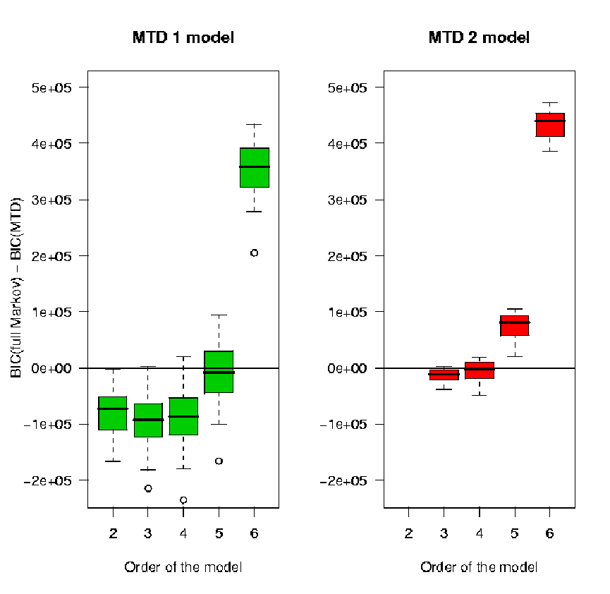
The full Markov model turns out to outperform the MTD₁ model when the order is inferior to 4. This is not surprising since the estimation is computed over large datasets that provide a sufficient amount of information with respect to the number of parameters of the full model. However, the 5^th order MTD₁ model and full Markov model have comparable performances, and the MTD₁ model outperforms the full Markov model for higher orders. This is an evidence that although MTD₁ only approximate the full Markov models, their estimation accuracy decreases slower with the order.

Even more striking is the comparison of the MTD₂ model with the full Markov model. Whatever the order of the model, its goodness-of-fit is at least equivalent to the one achieved by the full Markov model. The MTD_l model turns out to be a satisfactory trade-off between dimension and estimation accuracy.

5 Acknowledgments

We thank Bernard Prum and Catherine Matias for their very constructive suggestions, and Vincent Miele for his implementation of the EM algorithm in the seq++ library. Moreover, we thank the referees for their comments and suggestions which improve this paper.

Appendix A Example of equivalent parameters defining the same MTD₁ model

Let the size state space be 4 as for DNA sequences $\mathcal{Y}=\{a,c,g,t\}$ and consider these two $2^{nd}$ order MTD₁ model parameters $\bm{\theta},\bm{\theta}^{\prime}$ .

\begin{array}[]{lccc}\bm{\varphi}=(0.3,0.7)&\bm{\pi}_{1}=\left(\begin{array}[]{cccc}0.1&0.2&0.3&0.4\\ 0.4&0.3&0.2&0.1\\ 0.2&0.2&0.2&0.4\\ 0.4&0.2&0.2&0.2\end{array}\right)&\bm{\pi}_{2}=\left(\begin{array}[]{cccc}0.1&0.1&0.1&0.7\\ 0.2&0.2&0.4&0.2\\ 0.3&0.3&0.3&0.1\\ 0.3&0.2&0.3&0.2\end{array}\right)\\ &&\\ \bm{\varphi}^{\prime}=(0.2,0.8)&\bm{\pi}_{1}^{\prime}=\left(\begin{array}[]{cccc}0.2&0.1&0.2&0.5\\ 0.65&0.25&0.05&0.05\\ 0.35&0.1&0.05&0.5\\ 0.65&0.1&0.05&0.2\end{array}\right)&\bm{\pi}_{2}^{\prime}=\left(\begin{array}[]{cccc}0.075&0.1375&0.15&0.6375\\ 0.1625&0.225&0.4125&0.2\\ 0.25&0.3125&0.325&0.1125\\ 0.25&0.225&0.325&0.2\end{array}\right)\par\end{array}

Both parameters define the same $2^{nd}$ order Markov transition matrix $\bm{\Pi}$ .

\begin{array}[]{cc}&a\hskip 19.91684ptc\hskip 19.91684ptg\hskip 19.91684ptt\\ \bm{\Pi}=\begin{array}[]{l}aa\\ ac\\ ag\\ at\\ ca\\ cc\\ cg\\ ct\\ ga\\ gc\\ gg\\ gt\\ ta\\ tc\\ tg\\ tt\end{array}&\left(\begin{array}[]{cccc}0.1&0.13&0.16&0.61\\ 0.19&0.16&0.13&0.52\\ 0.13&0.13&0.13&0.61\\ 0.19&0.13&0.13&0.55\\ 0.17&0.2&0.37&0.26\\ 0.26&0.23&0.34&0.17\\ 0.2&0.2&0.34&0.26\\ 0.26&0.2&0.34&0.2\\ 0.24&0.27&0.3&0.19\\ 0.33&0.3&0.27&0.1\\ 0.27&0.27&0.27&0.19\\ 0.33&0.27&0.27&0.13\\ 0.24&0.2&0.3&0.26\\ 0.33&0.23&0.27&0.17\\ 0.27&0.2&0.27&0.26\\ 0.33&0.2&0.27&0.2\end{array}\right)\end{array}

Appendix B EM algorithm for other MTD models

B.1 Single matrix MTD model: iteration k.

E-Step

$\forall g\in\{1,...,m\},\forall\ i_{m},...,i_{1},i_{0}\in\{1,...,q\},$ P_S^(k)(g —i_m^0) = φ g (k) π (k) (i g ,i 0 ) ∑ l=1 m φ l (k) π (k) (i l ,i 0 ) .

M-Step

$\forall g\in\{1,...,m\},\forall i,j\in\{1,...,q\}$ ,

	$\displaystyle\varphi_{g}^{(k+1)}\!\!$	$\displaystyle=$	$\displaystyle\!\!\frac{1}{n-m}\sum_{i_{m}...i_{0}}\mathbb{P}^{(k)}(g\|\bm{i}_{m}^{0})N(\bm{i}_{m}^{0})$
	$\displaystyle\bm{\pi}^{(k+1)}(i,j)\!\!$	$\displaystyle=$	$\displaystyle\!\!\frac{\sum_{g=1}^{m}\sum_{i_{m}...i_{g+1}i_{g-1}...i_{1}}\mathbb{P}^{(k)}(g\|\bm{i}_{m}^{g+1}i\bm{i}_{g-1}^{1}j)N(\bm{i}_{m}^{g+1}i\bm{i}_{g-1}^{1}j)}{\sum_{g=1}^{m}\sum_{i_{m}...i_{g+1}i_{g-1}...i_{1}i_{0}}\mathbb{P}^{(k)}(g\|\bm{i}_{m}^{g+1}i\bm{i}_{g-1}^{0})N(\bm{i}_{m}^{g+1}i\bm{i}_{g-1}^{0})}$

where sums are carried out for the variables $i_{m},...,i_{g+1},i_{g-1},...,i_{1},i_{0}$ varying from $1$ to $q$ , $n$ is the length of the observed sequence $y$ and $N(\bm{i}_{m}^{0})$ the number of occurrences of the word $\bm{i}_{m}^{0}$ in this sequence.

B.2 MTD_l model: iteration k.

E-Step

$\forall g\in\{1,...,m-l+1\},\forall i_{m},...i_{1},i_{0}\in\{1,...,q\},$ P_S^(k)(g —i_m^0)= φ g (k) π g (k) (i g+l-1 g ,i 0 ) ∑ h=1 m-l+1 φ h (k) π h (k) (i h+l-1 h ,i 0 ) .

M-Step

$\forall g\in\{1,...,m\},\forall i_{l},...,i_{1},j\in\{1,...,q\}$ ,

	$\displaystyle\varphi_{g}^{(k+1)}\!\!$	$\displaystyle=$	$\displaystyle\!\!\frac{1}{n-m}\sum_{u_{m}...u_{0}}\mathbb{P}_{S}^{(k)}(g\|\bm{u}_{m}^{0})N(\bm{u}_{m}^{0})$
	$\displaystyle\bm{\pi}_{g}^{(k+1)}(i_{l}i_{l-1}...i_{1},j)\!\!$	$\displaystyle=$	$\displaystyle\!\!\frac{\sum_{u_{m}...u_{g+l}u_{g-1}...u_{1}}\mathbb{P}_{S}^{(k)}(g\|\bm{u}_{m}^{g+l}\bm{i}_{l}^{1}\bm{u}_{g-1}^{1}j)N(\bm{u}_{m}^{g+l}\bm{i}_{l}^{1}\bm{u}_{g-1}^{1}j)}{\sum_{u_{m}...u_{g+l}u_{g-1}...u_{1}u_{0}}\mathbb{P}_{S}(g\|\bm{u}_{m}^{g+l}\bm{i}_{l}^{1}\bm{u}_{g-1}^{0})N(\bm{u}_{m}^{g+l}\bm{i}_{l}^{1}\bm{u}_{g-1}^{0})},$

where sums are carried out for the variables $u_{m},...,u_{g+l},u_{g-1},...,u_{1},u_{0}$ varying from $1$ to $q$ , $n$ is the length of the observed sequence $y$ and $N(\bm{i}_{m}^{0})$ the number of occurrences of the word $\bm{i}_{m}^{0}$ in this sequence.

Appendix C $2^{nd}$ order MTD₁ estimates obtained on both the song of wood pewee and the mouse $\alpha$ A-Crystallin Gene sequence (Section 4.1).

Song of wood pewee

Berchtold’s algorithm (see [2], section 5.1): $L_{y}(\hat{\bm{\theta}})=-486.4$ .

\begin{array}[]{lccc}\hat{\bm{\varphi}}=(0.269,0.731)&\hat{\bm{\pi}}_{1}=\left(\begin{array}[]{ccc}0.097&0.739&0.164\\ 0.980&0&0.020\\ 0.987&0.013&0\end{array}\right)&\hat{\bm{\pi}}_{2}=\left(\begin{array}[]{ccc}0.996&0&0.004\\ 0.152&0.020&0.828\\ 0.003&0.997&0\end{array}\right).\\ \end{array}

EM-algorithm: $L_{y}(\hat{\bm{\theta}})=-481.8)$ .

\begin{array}[]{lccc}\hat{\bm{\varphi}}=(0.275,0.725)&\hat{\bm{\pi}}_{1}=\left(\begin{array}[]{ccc}0.102&0.729&0.169\\ 0.969&0&0.031\\ 0.987&0.013&0\end{array}\right)&\hat{\bm{\pi}}_{2}=\left(\begin{array}[]{ccc}1&0&0\\ 0.151&0.015&0.834\\ 0&1&0\end{array}\right).\\ \end{array}

These estimated parameters define respectively the following $2^{nd}$ order Markov transition matrices $\hat{\bm{\Pi}}_{B}$ and $\hat{\bm{\Pi}}_{EM}$ .

\begin{array}[]{cc}\hat{\bm{\Pi}}_{B}=\!\!\left(\begin{array}[]{lll}0.754169&0.198791&0.047040\\ 0.991696&0.&0.008304\\ 0.993579&0.003497&0.02924\\ 0.137205&0.213411&0.649384\\ 0.374732&0.01462&0.610648\\ 0.376615&0.018117&0.605268\\ 0.028286&0.927598&0.044116\\ 0.265813&0.728807&0.00538\\ 0.267696&0.732304&0.\end{array}\right)&\hat{\bm{\Pi}}_{EM}\!=\!\!\left(\begin{array}[]{lll}0.75305&0.200475&0.046475\\ 0.991475&0.&0.008525\\ 0.996425&0.003575&0.\\ 0.137525&0.21135&0.651125\\ 0.37595&0.010875&0.613175\\ 0.3809&0.01445&0.60465\\ 0.02805&0.925475&0.046475\\ 0.266475&0.725&0.008525\\ 0.271425&0.728575&0.\end{array}\right)\par\end{array}

Mouse $\alpha$ A-Crystallin Gene sequence

EM-algorithm: $L_{y}(\hat{\bm{\theta}})=-1718.5$ .

\hat{\bm{\varphi}}=(0.562,0.438),

\begin{array}[]{ccc}\hat{\bm{\pi}}_{1}=\left(\begin{array}[]{cccc}0.225&0.140&0.506&0.129\\ 0.354&0.300&0.008&0.338\\ 0.271&0.123&0.456&0.150\\ 0.166&0.191&0.430&0.213\end{array}\right)&\hat{\bm{\pi}}_{2}=\left(\begin{array}[]{cccc}0.094&0.600&0.149&0.157\\ 0.335&0.271&0.153&0.241\\ 0.185&0.415&0.099&0.301\\ 0.192&0.370&0.129&0.309\end{array}\right).\\ \end{array}

These estimated parameters define respectively the following $2^{nd}$ order Markov transition matrix $\hat{\bm{\Pi}}_{EM}$ .

\begin{array}[]{c}\hat{\bm{\Pi}}_{EM}\!=\!\!\left(\begin{array}[]{llll}0.167622&0.341480&0.349634&0.141264\\ 0.240120&0.431400&0.069758&0.258722\\ 0.193474&0.331926&0.321534&0.153066\\ 0.134464&0.370142&0.306922&0.188472\\ 0.273180&0.197378&0.351386&0.178056\\ 0.345678&0.287298&0.071510&0.295514\\ 0.299032&0.187824&0.323286&0.189858\\ 0.240022&0.226040&0.308674&0.225264\\ 0.207480&0.260450&0.327734&0.204336\\ 0.279978&0.350370&0.047858&0.321794\\ 0.233332&0.250896&0.299634&0.216138\\ 0.174322&0.289112&0.285022&0.251544\\ 0.210546&0.240740&0.340874&0.207840\\ 0.283044&0.330660&0.060998&0.325298\\ 0.236398&0.231186&0.312774&0.219642\\ 0.177388&0.269402&0.298162&0.255048\end{array}\right)\par\end{array}

No detail on the $2^{nd}$ order MTD₁ estimates from the mouse $\alpha$ A-Crystallin Gene sequence is given in [2].

References

[1] Berchtold, A. (1995). Autoregressive modeling of markov chains. In Statistical Modelling: Proceedings of the $10^{th}$ International Workshop on Statistical Modelling, pages 19–26. Springer-Verlag.
[2] Berchtold, A. (2001). Estimation in the mixture transition distribution model. Journal of Time Series Analysis, 22(4), 379–397.
[3] Berchtold, A. and Raftery, A. E. (2002). The mixture transition distribution model for high-order markov chains and non-gaussian time series. Statistical Science, 17, 328–356.
[4] Bühlmann, P. and Wyner, A. (1999). Variable length markov chains. Annals of Statistics, 27.
[5] Dempster, A., Laird, N., and Rubin, D. (1977). Maximum likelihood from incomplete data via the em algorithm. Journal of the Royal Statistical Society. Series B., 39, 1–38.
[6] Durbin, R., Eddy, S. R., Krogh, A., and Mitchison, G. (1999). Biological Sequence Analysis: Probabilistic Models of Proteins and Nucleic Acids. Cambridge University Press.
[7] Fichant, G. and Gautier, C. (1987). Statistical method for predicting protein coding regions in nucleic acid sequences. Computer applications in the biosciences : CABIOS., 3, 287–295.
[8] Grelot, A. (2005). Estimation Bayésienne d’un modèle MTD - MSc Report available at
http://stat.genopole.cnrs.fr/sg/Members/slebre/rapportAdeline.pdf/view.
[9] Lauritzen, S. L. (1998). Graphical models. Repr. Oxford Statistical Science Series. 17.
[10] Li, W. and Kwok, M. C. (1990). Some results on the estimation of a higher order markov chain. Commun. Stat. Simulat., 19(1), 363–380.
[11] Raftery, A. E. (1985). A model for high-order Markov chains. Journal of the Royal Statistical Society. Series B, 47(3), 528–539.
[12] Raftery, A. E. and Tavaré, S. (1994). Estimation and modelling repeated patterns in high order markov chains with the mixture transition distribution model. Journal of the Royal Statistical Society Applied Statistics, 43(1), 179–199.
[13] Schwarz, G. (1978). Estimating the dimension of a model. Annals of Statistics, 6(2), 461–464.
[14] Wu, C. (1983). On the convergence properties of the em algorithm. The Annals of Statistics, 11(1), 95–103.

	$\displaystyle Q(\bm{\theta}\|\bm{\theta}^{\prime})$	$\displaystyle=$	$\displaystyle\mathbb{E}\left[\log\mathbb{P}_{\bm{\theta}}(\bm{Y},\bm{S})\|\bm{Y}=\bm{y},\bm{\theta}^{\prime}\right]$
	$\displaystyle H(\bm{\theta}\|\bm{\theta}^{\prime})$	$\displaystyle=$	$\displaystyle\mathbb{E}\left[\log\mathbb{P}_{\bm{\theta}}(\bm{Y},\bm{S}\|\bm{Y}=\bm{y})\|\bm{y},\bm{\theta}^{\prime}\right]$

An EM algorithm for estimation in the Mixture Transition Distribution model

Abstract

1 Introduction

Need for parsimony

MTD modeling

Definition 1

Definition 2

Trade-off between dimension and maximal likelihood

The question of estimation

Berchtold’s Algorithm

2 Upper bound of the MTD model dimension

Proposition 1

Proposition 2

3 Estimation

3.1 Introduction of a hidden process

3.2 EM algorithm

E-step

M-Step

Initialization

EM-Algorithm for MTD models

4 Applications

4.1 Comparison with Berchtold’s Estimation

4.2 Estimation on DNA coding sequences

5 Acknowledgments

Appendix A Example of equivalent parameters defining the same MTD1 model

Appendix B EM algorithm for other MTD models

B.1 Single matrix MTD model: iteration k.

E-Step

M-Step

B.2 MTDl model: iteration k.

E-Step

M-Step

Appendix C 2n​d2^{nd} order MTD1 estimates obtained on both the song of wood pewee and the mouse α\alphaA-Crystallin Gene sequence (Section 4.1).

References

Appendix A Example of equivalent parameters defining the same MTD₁ model

B.2 MTD_l model: iteration k.

Appendix C $2^{nd}$ order MTD₁ estimates obtained on both the song of wood pewee and the mouse $\alpha$ A-Crystallin Gene sequence (Section 4.1).