跳到论文正文
W Papers独立论文阅读器 arXiv:0803.0524 论文正文 计算阅读时间 · 0%
引用这篇论文根据当前论文元数据生成,正式投稿前建议核对。


License: arXiv.org perpetual non-exclusive license
arXiv:0803.0524v1 [math.OC] 04 Mar 2008

Average performance of the sparsest approximation using a general dictionary

François Malgouyres⋆  and  Mila Nikolova⋄
⋆ LAGA/L2TI, Université Paris 13, CNRS, 99 avenue J.B. Clément, 93430 Villetaneuse, France;
(33/0) 1-49-40-35-83, malgouy@math.univ-paris13.fr
⋄ CMLA, ENS Cachan, CNRS, PRES UniverSud, 61 Av. President Wilson, F-94230 Cachan, France
(33/0) 1 47 50 59 08 nikolova@cmla.ens-cachan.fr
 
August 24, 2026
Abstract

We consider the minimization of the number of non-zero coefficients (the ℓ0\ell_{0} “norm”) of the representation of a data set in terms of a dictionary under a fidelity constraint. (Both the dictionary and the norm defining the constraint are arbitrary.) This (nonconvex) optimization problem naturally leads to the sparsest representations, compared with other functionals instead of the ℓ0\ell_{0} “norm”.

Our goal is to measure the sets of data yielding a KK-sparse solution—i.e. involving KK non-zero components. Data are assumed uniformly distributed on a domain defined by any norm—to be chosen by the user. A precise description of these sets of data is given and relevant bounds on the Lebesgue measure of these sets are derived. They naturally lead to bound the probability of getting a KK-sparse solution. We also express the expectation of the number of non-zero components. We further specify these results in the case of the Euclidean norm, the dictionary being arbitrary.

Key words: compression; approximation ; best K-term approximation; constrained minimization; dictionary; ℓ0\ell_{0} norm; estimation; frames; measure theory; nonconvex functions; sparse representations.

AMS class: 41A25, 41A29, 41A45, 41A50, 41A63.

1 Introduction

1.1 The problem under consideration

Our goal is to represent observed data d∈ℝNd\in\mathbb{R}^{N} in a economical way using a dictionary (ψi)i∈I(\psi_{i})_{i\in I} on ℝN\mathbb{R}^{N}, where II is a finite set of indexes and

span⁡{ψi:i∈I}=ℝN.\Span\big\{\psi_{i}:i\in I\big\}=\mathbb{R}^{N}. (1)

We study the sparsest representation where the (unknown) coefficients (λi)i∈I(\lambda_{i})_{i\in I} are estimated by solving the constraint optimization problem (𝒫d)({\mathcal{P}}_{d}) given below:

(𝒫d):{minimize(λi)i∈I​ℓ0​((λi)i∈I),under the constraint : ‖∑i∈Iλiψi−d‖≤τ,({\mathcal{P}}_{d}):~~~~~~~~~~~~~~~~~~~~\left\{\begin{array}[]{l}{\displaystyle\mbox{\rm minimize}_{(\lambda_{i})_{i\in I}}}\ell_{0}\big((\lambda_{i})_{i\in I}\big),\\ \mbox{under the constraint~: ~~}\left\|{\displaystyle\sum_{i\in I}}\lambda_{i}\psi_{i}-d\right\|\leq\tau,\end{array}\right.~~~~~~~~~~~~~~~~~~~~~~~~~~~~~~~~ (2)

with

ℓ0​((λi)i∈I)=def#⁡{i∈I:λi≠0},\ell_{0}((\lambda_{i})_{i\in I})\stackrel{{\scriptstyle\rm def}}{{=}}\#\big\{i\in I:\lambda_{i}\neq 0\big\},

where #\# stands for cardinality, ∥.∥\|.\| is an arbitrary norm and τ>0\tau>0 is a fixed parameter. Let us emphasize that for any d∈ℝNd\in\mathbb{R}^{N}, the constraint in (𝒫d)({\mathcal{P}}_{d}) is nonempty thanks to (1) and that the minimum is reached since ℓ0\ell_{0} takes its values in the finite set {0,1,…,#​I}\{0,1,\ldots,\#I\}.

Given the data dd, the norm ∥.∥\|.\|, the parameter τ\tau and the dictionary, the solution of (𝒫d)({\mathcal{P}}_{d}) is the sparsest possible, since the objective function ℓ0\ell_{0} in (2) minimizes the number of all non-zero coefficients in the set (λi)i∈I(\lambda_{i})_{i\in I} without penalizing them.

The function ℓ0\ell_{0} is sometimes abusively called the ℓ0\ell_{0}-norm. It can equivalently be written as

∑i∈Iφ⁡(λi)​where​φ​(t)={0ift=01ift≠0\sum_{i\in I}\varphi(\lambda_{i})~~~\mbox{where}~~~\varphi(t)=\left\{\begin{array}[]{ccc}0&\mbox{if}&t=0\\ 1&\mbox{if}&t\neq 0\end{array}\right. (3)

The function φ\varphi is discontinuous at zero and 𝒞∞{\mathcal{C}}^{\infty} beyond the origin, and has a long history. It was used in the context of Markov random fields by Geman and Geman 1984, cf. [8] and Besag 1986 [1] as a prior in MAP energies to restore labeled images (i.e. each λi\lambda_{i} belonging to a finite set of values):

ℰ⁡(λ)=‖∑i∈Iλi​ψi−d‖22+β​∑i∼jφ⁡(λi−λj),{\mathcal{E}}(\lambda)=\big\|\sum_{i\in I}\lambda_{i}\psi_{i}-d\big\|_{2}^{2}+\beta\sum_{i\sim j}\varphi(\lambda_{i}-\lambda_{j}), (4)

where the last term in (4) counts the number of all pairs of dissimilar neighbors ii and jj, and β>0\beta>0 is a parameter. This label-designed form is known as the Potts prior model, or as the multi-level logistic model [2, 11]. Guided by the Minimum description length principle of Rissanen, Y. Leclerc proposed in 1989 in [10] the same prior to restore piecewise constant, real-valued images. The hard-thresholding method to restore noisy wavelet coefficients, proposed by Donoho and Johnstone in 1992, see [6], amounts to minimize for each coefficient λi\lambda_{i} a function of the form ‖λi−gi‖22+β​φ​(λi)\|\lambda_{i}-g_{i}\|_{2}^{2}+\beta\varphi(\lambda_{i}) where the noisy coefficients read gi=⟨ψi∗,d⟩g_{i}=\langle\psi_{i}^{*},d\rangle, ∀i∈I\forall i\in I where (ψi)i∈I(\psi_{i})_{i\in I} is a wavelet basis. Very recently, the energy (4) was successfully used to reconstruct 3D tomographic images by using stochastic continuation by Robini and Magnin [19]. Let us notice that even though the problem (𝒫d)({\mathcal{P}}_{d}) in (2) and the minimization of ℰ{\mathcal{E}} in (4) are closely related, there is no rigorous equivalence in general.

The context of digital image compression is of a particular interest, since it is typically the problem we are modeling in the paper. In compression, one considers different classes of images. Those digital images live in ℝN\mathbb{R}^{N} and are obtained by sampling an analogue image. Their distribution in ℝN\mathbb{R}^{N} is one of the main unknown in image processing and, in practice, we only know some realizations of this distribution (i.e. some images). Given this (unknown) distribution, the goal of image compression is to build a coder (that encodes elements of ℝN\mathbb{R}^{N}) which assigns a small code to images. Typically, we want for every image d∈ℝNd\in\mathbb{R}^{N}

ℙ⁡(l​e​n​g​t​h​(c​o​d​e​(d))=K)\mathbb{P}\left(length(code(d))=K\right)

to be as large as possible for KK small, and small for KK large. We also want the decoder to satisfy d​e​c​o​d​e​(c​o​d​e​(d))∼ddecode(code(d))\sim d.

The link with the problem (𝒫d)({\mathcal{P}}_{d}), in (2), is that the current image compression standards (JPEG, JPEG2000) encode quantized versions of the coordinates of the image in a given basis. Moreover, most of the gain is made by choosing a basis such that the number of non-zero coordinates (after the quantization process) is small ([9, 20]). That is, we want to solve (𝒫d)({\mathcal{P}}_{d}) for each λi\lambda_{i} belonging to a finite set of values and for a basis (ψi)i∈I(\psi_{i})_{i\in I}. This link between image compression and (𝒫d)({\mathcal{P}}_{d}) might seem restrictive when we only consider a basis. It makes much more sense when we consider a redundant system of vectors (ψi)i∈I(\psi_{i})_{i\in I}. The use of redundant dictionaries has known a strong development in the past years, see [4, 17, 18, 3] for the most famous examples. In the context of dictionaries, we know that the length of the code for encoding (λi)i∈I(\lambda_{i})_{i\in I} is in general proportional to ℓ0​((λi)i∈I)\ell_{0}((\lambda_{i})_{i\in I}). The problem (𝒫d)({\mathcal{P}}_{d}) therefore reads : minimize the codelength of the image while constraining a given level of accuracy of the coder. This is exactly the goal in image compression.

Finding an exact solution to (𝒫d)({\mathcal{P}}_{d}) in large dimension (which is necessary in order to apply (𝒫d)({\mathcal{P}}_{d}) to image compression) still remains a challenge. In fact, the methods described in [4, 18, 3] can be seen as heuristics approximating (𝒫d)({\mathcal{P}}_{d}). The links between the performances of those heuristics and the performances of (𝒫d)({\mathcal{P}}_{d}) is not completely clear. It is also a goal of the paper to provide a mean for comparing those algorithms.

1.2 Our contribution

In this paper, we estimate the ability of the model (𝒫d)({\mathcal{P}}_{d}) to provide a sparse representation of data which follows a given distribution law. The distribution law is uniform in the θ\theta-level set of a norm fdf_{d} :

ℒfd​(θ)={w∈ℝN,fd​(w)≤θ}.{\mathcal{L}}_{f_{d}}(\theta)=\{w\in\mathbb{R}^{N},f_{d}(w)\leq\theta\}.

In order to do this we

  • •

    Give a precise (and non redundant) geometrical description of the sets

    ℐτ​(K)={d∈ℝN,val⁡(𝒫d)≤K},{{\mathcal{I}}^{\tau}\left(K\right)}=\left\{d\in\mathbb{R}^{N},\val({\mathcal{P}}_{d})\leq K\right\},

    and

    𝒟τ​(K)={d∈ℝN,val⁡(𝒫d)=K}{{\mathcal{D}}^{\tau}\left(K\right)}=\left\{d\in\mathbb{R}^{N},\val({\mathcal{P}}_{d})=K\right\} (5)

    where val⁡(𝒫d)\val({\mathcal{P}}_{d}) denotes ℓ0​((λi)i∈I)\ell_{0}((\lambda_{i})_{i\in I}) for a solution (λi)i∈I(\lambda_{i})_{i\in I} of (𝒫d)({\mathcal{P}}_{d}) and for K=0,…,NK=0,\ldots,N, τ>0\tau>0. This is done in Theorem 1 and equation (69).

    Remark 1

    It is easy to see that {ψi:λi≠0​for​(λi)i∈I​solving​(𝒫d)}\Big\{\psi_{i}:\lambda_{i}\neq 0~\mbox{for}~(\lambda_{i})_{i\in I}~\mbox{\rm solving}~({\mathcal{P}}_{d})\Big\} forms a set of linearly independent vectors. Therefore for all d∈ℝd\in\mathbb{R} we will find a solution with at most NN nonzero coefficients, even if the size of the dictionary is huge, #​I≫N\#I\gg N. So in this work we consider solutions with sparsity K≤NK\leq N.

  • •

    Once these sets are precisely described, we are able to bound (both from above and from below), their measure (more precisely the measure of their intersection with ℒfd​(θ){\mathcal{L}}_{f_{d}}(\theta)). The difference between the upper and the lower bound is negligible when compared to (τθ)N−K\left(\frac{\tau}{\theta}\right)^{N-K}, when τθ\frac{\tau}{\theta} is mall enough. Moreover, these bounds show that the measures of ℐτ​(K)∩ℒfd​(θ){{\mathcal{I}}^{\tau}\left(K\right)}\cap{\mathcal{L}}_{f_{d}}(\theta) and 𝒟τ​(K)∩ℒfd​(θ){{\mathcal{D}}^{\tau}\left(K\right)}\cap{\mathcal{L}}_{f_{d}}(\theta) asymptotically behave like

    𝑪¯K​θN​(τθ)N−K,\mbox{\boldmath$\overline{C}$\unboldmath${}_{K}$}\theta^{N}\left(\frac{\tau}{\theta}\right)^{N-K},

    as τθ\frac{\tau}{\theta} goes to 00.

    The constants 𝑪¯\overline{C}K are defined in (44). They are made of the sum of constants CVC_{V} over all possible vector subspaces VV of dimension KK, spanned by elements of the dictionary (ψi)i∈I(\psi_{i})_{i\in I}. The constants CVC_{V} are built in Proposition 1 and Corollary 1. They have the form

    CV=𝕃N−K(PV⊥(ℒ∥.∥(1)))𝕃K(V∩ℒfd(1)),C_{V}={\mathbb{L}}^{{}^{{}_{\!\!N-K}}}\big(P_{V^{\bot}}\left({\mathcal{L}}_{\|.\|}(1)\right)\big){\mathbb{L}}^{{}^{{}_{\!\!K}}}\big(V\cap{\mathcal{L}}_{f_{d}}(1)\big),

    where PV⊥P_{V^{\bot}} is the orthogonal projection onto the orthogonal complement of VV, ∥.∥\|.\| is the norm defining the data fidelity term in (𝒫d)({\mathcal{P}}_{d}) and 𝕃k(.){\mathbb{L}}^{{}^{{}_{\!\!k}}}\big(.\big) denotes the Lebesgue measure of a set living in ℝk\mathbb{R}^{k}.

  • •

    Once this is achieved, we easily obtain lower and upper bounds for ℙ⁡(val⁡(𝒫d)≤K)\mathbb{P}\left(\val({\mathcal{P}}_{d})\leq K\right), ℙ⁡(val⁡(𝒫d)=K)\mathbb{P}\left(\val({\mathcal{P}}_{d})=K\right) when dd is uniformly distributed in ℒfd​(θ){\mathcal{L}}_{f_{d}}(\theta) (see Section 6). They have the same characteristics as the bounds described above (modulo the disappearance of θN\theta^{N}). In order to obtain sparse representations of the data, we should therefore tune the model (the norm ∥.∥\|.\| and the dictionary (ψi)i∈I(\psi_{i})_{i\in I}) in order to obtain larger constants 𝑪¯\overline{C}K.

    This result clearly shows that the model (𝒫d)({\mathcal{P}}_{d}) benefits from several ingredient (which might not be present in other models promoting sparsity):

    • –

      the sum defining 𝑪¯\overline{C}K is for all the possible vector subspaces of dimension KK spanned by elements of the dictionary (ψi)i∈I(\psi_{i})_{i\in I}.

    • –

      the term 𝕃K(V∩ℒfd(1)){\mathbb{L}}^{{}^{{}_{\!\!K}}}\big(V\cap{\mathcal{L}}_{f_{d}}(1)\big) in in the constants CVC_{V} represents the measure of the whole set V∩ℒfd​(1)V\cap{\mathcal{L}}_{f_{d}}(1).

  • •

    Finally we estimate 𝔼⁡(val⁡(𝒫d))\mathbb{E}\left(\val({\mathcal{P}}_{d})\right) and show that its asymptotic (when τθ\frac{\tau}{\theta} goes to 00) is governed by the constant 𝑪¯\overline{C}N-1 (see Theorem 5). Increasing this constant therefore seems to be particularly important when building a model (𝒫d)({\mathcal{P}}_{d}) (i.e. choosing ∥.∥\|.\| and (ψi)i∈I(\psi_{i})_{i\in I}).

These results are illustrated in the context of particular choice for ∥.∥\|.\| and for fdf_{d} in Section 7.

1.3 Relation to other evaluations of performance

Evaluating the performance of an optimization problem like (𝒫d)({\mathcal{P}}_{d}) for the purpose of realizing nonlinear approximation is a very active firld of research. For a good survey of the problem we refer to [5].

In that field of research a variant of (𝒫d)({\mathcal{P}}_{d}), named “best K-term approximation”, is under study. It consists in looking for the best possible approximation of a datum d∈ℝNd\in\mathbb{R}^{N} using an expansion in (ψi)i∈I(\psi_{i})_{i\in I} with KK non-zero coordinates. The performance of the model is estimated using the quantity

σK​(d)=infS∈ΣK‖d−S‖,\sigma_{K}(d)=\inf_{S\in\Sigma_{K}}\|d-S\|,

where ΣK\Sigma_{K} denotes the union of all the vector spaces of dimension KK spanned by elements of (ψi)i∈I(\psi_{i})_{i\in I}, for K=0,…,NK=0,\ldots,N. Expressed with our notations, the typical object under consideration is11 1 In Nonlinear approximation authors usually consider infinite dimensional spaces.

𝒜α​(C)=⋃K=1N𝒟CKα​(K),{\mathcal{A}}^{\alpha}(C)=\bigcup_{K=1}^{N}{{\mathcal{D}}^{\frac{C}{K^{\alpha}}}\left(K\right)},

for C>0C>0 and α>0\alpha>0 and 𝒟τ​(K){{\mathcal{D}}^{\tau}\left(K\right)} defined by (5). That is the data dd obeying

σK(d)≤CKα, for all K=1,…,N.\sigma_{K}(d)\leq\frac{C}{K^{\alpha}}~~~~\mbox{, for all }K=1,\ldots,N.

The typical results obtained there take the form

𝒜α​(C1)⊂𝒦η⊂𝒜α​(C2),{\mathcal{A}}^{\alpha}(C_{1})\subset{\mathcal{K}}_{\eta}\subset{\mathcal{A}}^{\alpha}(C_{2}), (6)

for C2≥C1>0C_{2}\geq C_{1}>0 and the level set

𝒦η={d∈ℝN,‖d‖η≤1},{\mathcal{K}}_{\eta}=\{d\in\mathbb{R}^{N},\|d\|_{\eta}\leq 1\},

for a norm ∥.∥η\|.\|_{\eta} characterizing the regularity of dd (again, the theory is in infinite dimensional vector spaces). This permits to estimate the number of coordinates which are needed to represent a datum dd, if we know its regularity. Typically, the link between α\alpha and η\eta says how good is the basis (or more generally a dictionary) at representing the data class.

The clear advantage of these results over ours is that they apply even if one only has a vague knowledge of the data distribution. For instance, any data distribution whose support is included in 𝒦η{\mathcal{K}}_{\eta} does enjoy the decay C2Kα\frac{C_{2}}{K^{\alpha}}. The inclusions in (6) need indeed to be true for the worse elements of 𝒦η{\mathcal{K}}_{\eta} (even if they are rare). The counterpart of this advantage is that the constants C1C_{1} and C2C_{2} might be pessimistic.

Finally, as far as we know, the analysis proposed in Nonlinear approximation does not permit (today) to clearly assess the differences between (𝒫d)({\mathcal{P}}_{d}) and its heuristics (in particular Basis Pursuit Denoising [3] and Orthogonal Matching Pursuit [18]). This is a clear advantage of the method for assessing model performances proposed in this paper. Indeed, similar analysis have already been conducted in [16, 13, 15] in the context of the compression scheme described in [14], Basis Pursuit Denoising and total variation regularization. (However, concerning the papers on Basis Pursuit Denoising and the total variation regularization, the results are stated for another asymptotic and the analysis partly needs to be rewritten in the proper context.)

1.4 Notations

For any function f:ℝN→ℝf:\mathbb{R}^{N}\to\mathbb{R}, and any θ∈ℝ\theta\in\mathbb{R}, the θ\theta-level set of ff is denoted by

ℒf​(θ)={w∈ℝN,f⁡(w)≤θ}.{\mathcal{L}}_{f}(\theta)=\{w\in\mathbb{R}^{N},f(w)\leq\theta\}. (7)

For any vector subspace VV of ℝN\mathbb{R}^{N}, we denote PVP_{V} the orthogonal projection onto VV and by V⊥V^{\bot} the orthogonal complement of VV in ℝN\mathbb{R}^{N}. To specify the dimension of VV, we write dim(V)\dim(V). The Euclidean norm of an u∈ℝNu\in\mathbb{R}^{N} is systematically denoted by ‖u‖2\|u\|_{2}. The notation ‖u‖\|u\| is devoted to a general norm on ℝN\mathbb{R}^{N}. For any integer K>0K>0, the Lebesgue measure on ℝK\mathbb{R}^{K} is systematically denoted by 𝕃K(.){\mathbb{L}}^{{}^{{}_{\!\!K}}}\big(.\big), whereas IKI_{K} stands for the K×KK\times K identity matrix. We write ℙ(.)\mathbb{P}\left(.\right) for probability and 𝔼(.)\mathbb{E}\left(.\right) for expectation.

As usually, we write o⁡(t)o(t) for a function satisfying limt→0o⁡(t)t=0\lim_{t\to 0}\frac{o(t)}{t}=0.

For any d∈ℝNd\in\mathbb{R}^{N}, we denote val⁡(𝒫d)\val({\mathcal{P}}_{d}) the value of the minimum in (𝒫d)({\mathcal{P}}_{d})—i.e. ℓ0​((λi)i∈I)\ell_{0}\left((\lambda_{i})_{i\in I}\right) for (λi)i∈I(\lambda_{i})_{i\in I} solving (𝒫d)({\mathcal{P}}_{d}).

2 Measuring bounded cylinder-like subsets of ℝN\mathbb{R}^{N}

2.1 Preliminary results

Below we give several statements that will be used many times in the rest of the work.

Lemma 1

For any vector subspace V⊂ℝNV\subset\mathbb{R}^{N} and any norm ∥.∥\|.\| on ℝN\mathbb{R}^{N}, define the application

h:V⊥\displaystyle h:V^{\bot} →\displaystyle\to ℝ\displaystyle\mathbb{R}
u\displaystyle u →\displaystyle\to h(u)=definf{t≥0:ut∈PV⊥(ℒ∥.∥(1))}.\displaystyle h(u)\stackrel{{\scriptstyle\rm def}}{{=}}\inf\left\{t\geq 0:\frac{u}{t}\in P_{V^{\bot}}\left({\mathcal{L}}_{\|.\|}(1)\right)\right\}. (8)

Then the following holds:

  • (i)

    For any τ≥0\tau\geq 0, we have

    ℒh(τ)=PV⊥(ℒ∥.∥(τ)).{\mathcal{L}}_{h}(\tau)=P_{V^{\bot}}\left({\mathcal{L}}_{\|.\|}(\tau)\right). (9)
  • (ii)

    The application hh in (8) is a norm on V⊥V^{\bot}.

  • (iii)

    For any norm fdf_{d} on ℝN\mathbb{R}^{N}, let δ1>0\delta_{1}>0, δ2>0\delta_{2}>0 and Δ¯{\overline{\Delta}} be some constants satisfying

    w∈ℝN\displaystyle w\in\mathbb{R}^{N} ⇒\displaystyle\Rightarrow fd​(w)≤δ1​‖w‖2​ and ​‖w‖2≤δ2​‖w‖,\displaystyle f_{d}(w)\leq\delta_{1}\|w\|_{2}\mbox{~ and ~}\|w\|_{2}\leq\delta_{2}\|w\|, (10)
    Δ¯\displaystyle{\overline{\Delta}} =def\displaystyle\stackrel{{\scriptstyle\rm def}}{{=}} δ1​δ2\displaystyle\delta_{1}\delta_{2} (11)

    The constants δ1\delta_{1}, δ2\delta_{2} and Δ¯>0{\overline{\Delta}}>0 are independent of VV and we have

    fd​(u)\displaystyle f_{d}(u) ≤\displaystyle\leq Δ¯​h​(u),∀u∈V⊥,\displaystyle{\overline{\Delta}}h(u),~~~~~~\forall u\in V^{\bot}, (12)
    ‖u‖2\displaystyle\|u\|_{2} ≤\displaystyle\leq δ2​h​(u),∀u∈V⊥.\displaystyle\delta_{2}h(u),~~~~~~\forall u\in V^{\bot}. (13)
Remark 2

The constants in (10) come from the fact that all norms on a finite-dimensional space are equivalent. In practice we will choose the smallest constants satisfying these inequalities.

Proof. The case V={0}V=\{0\} is trivial (we obtain h=∥.∥h=\|.\|) and we further assume that dim(V)≥1\dim(V)\geq 1.

Assertion (i).

The set PV⊥(ℒ∥.∥(1))P_{V^{\bot}}({\mathcal{L}}_{\|.\|}(1)) is convex since ∥.∥\|.\| is a norm and PV⊥P_{V^{\bot}} is linear. Moreover, the origin 0 belongs to its interior. Indeed, there is ε>0\varepsilon>0 such that if w∈ℝNw\in\mathbb{R}^{N} satisfies ‖w‖2<ε\|w\|_{2}<\varepsilon, then ‖w‖<1\|w\|<1. Consequently 0∈Int(ℒ∥.∥2(ε))⊂ℒ∥.∥(1)0\in{\rm Int}\big({\mathcal{L}}_{\|.\|_{2}}(\varepsilon)\big)\subset{\mathcal{L}}_{\|.\|}(1). Using that ∥.∥2\|.\|_{2} is rotationally invariant and that PV⊥P_{V^{\bot}} is a contraction, we deduce that 0∈Int(PV⊥(ℒ∥.∥2(ε)))⊂PV⊥(ℒ∥.∥(1))0\in{\rm Int}\big(P_{V^{\bot}}({\mathcal{L}}_{\|.\|_{2}}(\varepsilon))\big)\subset P_{V^{\bot}}({\mathcal{L}}_{\|.\|}(1)). Then the application h:V⊥→ℝh:V^{\bot}\to\mathbb{R} in (8) is the usual Minkowski functional of PV⊥(ℒ∥.∥(1))P_{V^{\bot}}\left({\mathcal{L}}_{\|.\|}(1)\right), as defined and commented in [12, p.131]. Since PV⊥(ℒ∥.∥(1))P_{V^{\bot}}\left({\mathcal{L}}_{\|.\|}(1)\right) is closed, we have

PV⊥(ℒ∥.∥(1))={u∈V⊥:h(u)≤1}.P_{V^{\bot}}\left({\mathcal{L}}_{\|.\|}(1)\right)=\big\{u\in V^{\bot}:h(u)\leq 1\big\}.

Using that the Minkowski functional is positively homogeneous—i.e.

h⁡(τ​u)=τ​h​(u),∀τ>0,h(\tau u)=\tau h(u),~~~\forall\tau>0,

lead to (9).

Assertion (ii).

For hh to be a norm, we have to show that the latter property holds for any λ∈ℝ\lambda\in\mathbb{R} (i.e. that hh is symmetric with respect to the origin). It is true since, for any λ∈ℝ\lambda\in\mathbb{R}

h⁡(λ​u)\displaystyle~~~~~~~~~h(\lambda u) =\displaystyle= inf{t≥0:λu∈PV⊥(ℒ∥.∥(t))}\displaystyle\inf\big\{t\geq 0:\lambda u\in P_{V^{\bot}}\left({\mathcal{L}}_{\|.\|}(t)\right)\big\}
=\displaystyle= inf{t≥0:u∈PV⊥(ℒ∥.∥(t|λ|))}\displaystyle\inf\big\{t\geq 0:u\in P_{V^{\bot}}\left({\mathcal{L}}_{\|.\|}(\frac{t}{|\lambda|})\right)\big\}
=\displaystyle= |λ|inf{t≥0:u∈PV⊥(ℒ∥.∥(t))}(writing t for t/|λ|)\displaystyle|\lambda|\inf\big\{t\geq 0:u\in P_{V^{\bot}}\left({\mathcal{L}}_{\|.\|}(t)\right)\big\}~~~~~~~~~\mbox{(writing $t$ for $t/|\lambda|$)}
=\displaystyle= |λ|​h​(u),\displaystyle|\lambda|~h(u),

where we use the facts that PV⊥P_{V^{\bot}} is linear and that ∥.∥\|.\| is a norm. It is well known that the Minkowski functional is non negative, finite, and satisfies22 2 For completeness, we give the details: h⁡(u+v)\displaystyle h(u+v) =\displaystyle= inf{t≥0:(u+v)∈PV⊥(ℒ∥.∥(t))}\displaystyle\inf\big\{t\geq 0:(u+v)\in P_{V^{\bot}}\left({\mathcal{L}}_{\|.\|}(t)\right)\big\} ≤\displaystyle\leq inf{t≥0:u∈PV⊥(ℒ∥.∥(t))}+inf{t≥0:v∈PV⊥(ℒ∥.∥(t))}=h(u)+h(v).\displaystyle\inf\big\{t\geq 0:u\in P_{V^{\bot}}\left({\mathcal{L}}_{\|.\|}(t)\right)\big\}+\inf\big\{t\geq 0:v\in P_{V^{\bot}}\left({\mathcal{L}}_{\|.\|}(t)\right)\big\}=h(u)+h(v).   h⁡(u+v)≤h⁡(u)+h⁡(v)h(u+v)\leq h(u)+h(v) for any u,v∈V⊥u,v\in V^{\bot}.

Finally, since ℒh(0)=PV⊥(ℒ∥.∥(0))={0}{\mathcal{L}}_{h}(0)=P_{V^{\bot}}\left({\mathcal{L}}_{\|.\|}(0)\right)=\{0\},

h⁡(u)=0⇔u=0.h(u)=0~~~\Leftrightarrow~~~u=0.

Consequently, hh defines a norm on V⊥V^{\bot}.

Assertion (iii).

Let us first remark that

ℒ∥.∥(1)⊂ℒ∥.∥2(δ2)⊂ℒfd(δ1δ2)=ℒfd(Δ¯),{\mathcal{L}}_{\|.\|}(1)\subset{\mathcal{L}}_{\|.\|_{2}}(\delta_{2})\subset{\mathcal{L}}_{f_{d}}(\delta_{1}\delta_{2})={\mathcal{L}}_{f_{d}}({\overline{\Delta}}),

where δ1\delta_{1} and δ2\delta_{2} are defined in the proposition. Using that ∥.∥2\|.\|_{2} is rotationally invariant, we have

ℒh(1)=PV⊥(ℒ∥.∥(1))\displaystyle{\mathcal{L}}_{h}(1)=P_{V^{\bot}}\left({\mathcal{L}}_{\|.\|}(1)\right) ⊂\displaystyle\subset PV⊥(ℒ∥.∥2(δ2))=ℒ∥.∥2(δ2)∩V⊥\displaystyle P_{V^{\bot}}\left({\mathcal{L}}_{\|.\|_{2}}(\delta_{2})\right)={\mathcal{L}}_{\|.\|_{2}}(\delta_{2})\cap V^{\bot}
⊂\displaystyle\subset ℒfd​(δ1​δ2)∩V⊥=ℒfd​(Δ¯)∩V⊥.\displaystyle{\mathcal{L}}_{f_{d}}(\delta_{1}\delta_{2})\cap V^{\bot}={\mathcal{L}}_{f_{d}}({\overline{\Delta}})\cap V^{\bot}.

We will prove (12) and (13) jointly. To this end let us consider a norm gg on ℝN\mathbb{R}^{N} and δ>0\delta>0 such that

PV⊥(ℒ∥.∥(1))⊂ℒg(δ)∩V⊥.P_{V^{\bot}}\left({\mathcal{L}}_{\|.\|}(1)\right)\subset{\mathcal{L}}_{g}(\delta)\cap V^{\bot}. (14)

Using that each norm can be expressed as a Minkowski functional, for any u∈V⊥u\in V^{\bot} we can write down the following:

g⁡(u)\displaystyle g(u) =\displaystyle= inf{t≥0:g⁡(ut)≤1}\displaystyle\inf\{t\geq 0:g(\frac{u}{t})\leq 1\} (15)
=\displaystyle= inf{t≥0:g⁡(δt​u)≤δ}\displaystyle\inf\{t\geq 0:g(\frac{\delta}{t}u)\leq\delta\}
=\displaystyle= δ​inf{t≥0:g⁡(ut)≤δ}(write t for tδ)\displaystyle\delta\inf\{t\geq 0:g(\frac{u}{t})\leq\delta\}~~~~~~~~~~~~~\mbox{(write $t$ for $\frac{t}{\delta}$)}
=\displaystyle= δ​inf{t≥0:ut∈ℒg​(δ)}\displaystyle\delta\inf\{t\geq 0:\frac{u}{t}\in{\mathcal{L}}_{g}(\delta)\}
≤\displaystyle\leq δinf{t≥0:ut∈PV⊥(ℒ∥.∥(1)})\displaystyle\delta\inf\{t\geq 0:\frac{u}{t}\in P_{V^{\bot}}\left({\mathcal{L}}_{\|.\|}(1)\}\right)
≤\displaystyle\leq δ​h​(u),\displaystyle\delta~h(u),

where the inequality in (15) comes from (14).

If we identify gg with fdf_{d} and δ\delta with Δ¯{\overline{\Delta}}, we obtain (12). Similarly, identifying gg with ∥.∥2\|.\|_{2} and δ\delta with δ2\delta_{2} yields (13). This concludes the proof. □\Box

The next proposition addresses sets of ℝN\mathbb{R}^{N} bounded with the aid of fdf_{d}.

Proposition 1

For any vector subspace VV of ℝN\mathbb{R}^{N}, any norm ∥.∥\|.\| on ℝN\mathbb{R}^{N} and any τ>0\tau>0, define

Vτ=V+PV⊥(ℒ∥.∥(τ)).V^{\tau}=V+P_{V^{\bot}}\left({\mathcal{L}}_{\|.\|}(\tau)\right). (16)

Then the following hold:

  • (i)

    VτV^{\tau} is closed and measurable;

  • (ii)

    Let fdf_{d} be any norm on ℝN\mathbb{R}^{N}, h:V⊥→ℝh:V^{\bot}\to\mathbb{R} the norm defined in Lemma 1, K=dim(V)K=\dim(V) and δV\delta_{V} be any constant such that

    fd(u)≤δVh(u),∀u∈V⊥.f_{d}(u)\leq\delta_{{}_{V}}h(u),~~~\forall u\in V^{\bot}. (17)

    If  θ≥δVτ\theta\geq\delta_{{}_{V}}\tau, then

    CτN−K(θ−δVτ)K≤𝕃N(Vτ∩ℒfd(θ))≤CτN−K(θ+δVτ)K,C\tau^{N-K}(\theta-\delta_{{}_{V}}\tau)^{K}\leq{\mathbb{L}}^{{}^{{}_{\!\!N}}}\big(V^{\tau}\cap{\mathcal{L}}_{f_{d}}(\theta)\big)\leq C\tau^{N-K}(\theta+\delta_{{}_{V}}\tau)^{K}, (18)

    where

    C=𝕃N−K(PV⊥(ℒ∥.∥(1)))𝕃K(V∩ℒfd(1))∈(0,+∞).C={\mathbb{L}}^{{}^{{}_{\!\!N-K}}}\big(P_{V^{\bot}}\left({\mathcal{L}}_{\|.\|}(1)\right)\big)~{\mathbb{L}}^{{}^{{}_{\!\!K}}}\big(V\cap{\mathcal{L}}_{f_{d}}(1)\big)~\in~(0,+\infty). (19)
Remark 3

Using Lemma 1, the condition in (17) holds for any δV≥δV∗\delta_{V}\geq\delta_{V}^{*} with δV∗∈[0,Δ¯]\delta_{V}^{*}\in[0,{\overline{\Delta}}], where Δ¯{\overline{\Delta}} is given in (11). Let us emphasize that δV\delta_{V} may depend on VV (which explains the letter “V” in index). The proposition clearly holds if we take δV=Δ¯\delta_{V}={\overline{\Delta}}—the constant of Lemma 1, assertion (iii), which is independent of the choice of VV.

Observe that CC is a positive, finite constant that depends only on VV, ∥.∥\|.\| and fdf_{d}.

Remark 4

An important consequence of this proposition is that asymptotically

𝕃N(Vτ∩ℒfd(θ))=CθN(τθ)N−K+θNo((τθ)N−K)ifτθ→0.{\mathbb{L}}^{{}^{{}_{\!\!N}}}\big(V^{\tau}\cap{\mathcal{L}}_{f_{d}}(\theta)\big)=C\theta^{N}\left(\frac{\tau}{\theta}\right)^{N-K}+\theta^{N}o\left(\left(\frac{\tau}{\theta}\right)^{N-K}\right)~~~\mbox{if}~~~\frac{\tau}{\theta}\to 0.

Proof. The sets VV and PV⊥(ℒ∥.∥(τ))P_{V^{\bot}}\left({\mathcal{L}}_{\|.\|}(\tau)\right) are closed. Moreover, VV and PV⊥(ℒ∥.∥(τ))P_{V^{\bot}}\left({\mathcal{L}}_{\|.\|}(\tau)\right) are orthogonal. Therefore VτV^{\tau} is closed. As a consequence VτV^{\tau} is a Borel set and is Lebesgue measurable.

Since the restriction of fdf_{d} to V⊥V^{\bot} is a norm on V⊥V^{\bot}, there exists δV\delta_{V} such that (see Remark 2)

fd(u)≤δVh(u),∀u∈V⊥,f_{d}(u)\leq\delta_{{}_{V}}h(u),~~~\forall u\in V^{\bot}, (20)

where hh is given in (9) in Lemma 1. By (12) in Lemma 1, such a δV\delta_{V} exists in [0,Δ¯][0,{\overline{\Delta}}]. To simplify the notations, in the rest of the proof we will write δ\delta for δV\delta_{{}_{V}}.

For any u∈V⊥u\in V^{\bot} and v∈Vv\in V, using (20) we have

fd​(v)−δ​h​(u)≤fd​(v)−fd​(u)≤fd​(u+v)≤fd​(v)+fd​(u)≤fd​(v)+δ​h​(u)f_{d}(v)-\delta h(u)\leq f_{d}(v)-f_{d}(u)\leq f_{d}(u+v)\leq f_{d}(v)+f_{d}(u)\leq f_{d}(v)+\delta h(u)

In particular, for h⁡(u)≤τh(u)\leq\tau, we get

fd​(v)−δ​τ≤fd​(u+v)≤fd​(v)+δ​τ.f_{d}(v)-\delta\tau\leq f_{d}(u+v)\leq f_{d}(v)+\delta\tau. (21)

As required in assertion (ii), we have θ−δ​τ≥0\theta-\delta\tau\geq 0. If in addition v∈Vv\in V is such that fd​(v)≤θ−δ​τf_{d}(v)\leq\theta-\delta\tau, then fd​(u+v)≤θf_{d}(u+v)\leq\theta. Noticing that

ℒfd(θ)={u+v:(u,v)∈(V⊥×V),fd(u+v)≤θ},{\mathcal{L}}_{f_{d}}(\theta)=\big\{u+v:(u,v)\in(V^{\bot}\!\!\times V),~f_{d}(u+v)\leq\theta\big\},

this implies that

B0=def{u+v:(u,v)∈(V⊥×V),h(u)≤τ,fd(v)≤θ−δτ}⊆Vτ∩ℒfd(θ).B_{0}\stackrel{{\scriptstyle\rm def}}{{=}}\big\{u+v:(u,v)\in(V^{\bot}\!\!\times V),~h(u)\leq\tau,~f_{d}(v)\leq\theta-\delta\tau\big\}~\subseteq~V^{\tau}\cap{\mathcal{L}}_{f_{d}}(\theta).

Using that fd​(u+v)≤θf_{d}(u+v)\leq\theta (see the set we wish to measure in (18)), then the left-hand side of (21) shows that fd​(v)≤θ+δ​τf_{d}(v)\leq\theta+\delta\tau, hence

B1=def{u+v:(u,v)∈(V⊥×V),h(u)≤τ,fd(v)≤θ+δτ}⊇Vτ∩ℒfd(θ).B_{1}\stackrel{{\scriptstyle\rm def}}{{=}}\big\{u+v:(u,v)\in(V^{\bot}\!\!\times V),~h(u)\leq\tau,~f_{d}(v)\leq\theta+\delta\tau\big\}~\supseteq~V^{\tau}\cap{\mathcal{L}}_{f_{d}}(\theta).

Consider the pair of applications

φ0:ℒh​(1)×(V∩ℒfd​(1))\displaystyle\varphi_{0}:{\mathcal{L}}_{h}(1)\times\left(V\cap{\mathcal{L}}_{f_{d}}(1)\right) →\displaystyle\to ℝN\displaystyle\mathbb{R}^{N}
(u,v)\displaystyle(u,v) →\displaystyle\to τ​u+(θ−δ​τ)​v\displaystyle\tau u+(\theta-\delta\tau)v

and

φ1:ℒh​(1)×(V∩ℒfd​(1))\displaystyle\varphi_{1}:{\mathcal{L}}_{h}(1)\times\left(V\cap{\mathcal{L}}_{f_{d}}(1)\right) →\displaystyle\to ℝN\displaystyle\mathbb{R}^{N}
(u,v)\displaystyle(u,v) →\displaystyle\to τ​u+(θ+δ​τ)​v\displaystyle\tau u+(\theta+\delta\tau)v

Clearly, φi\varphi_{i} is a Lipschitz homeomorphism satisfying φi​(ℒh​(1)×(V∩ℒfd​(1)))=Bi\varphi_{i}\Big({\mathcal{L}}_{h}(1)\times\big(V\cap{\mathcal{L}}_{f_{d}}(1)\big)\Big)=B_{i} for i∈{0,1}i\in\{0,~1\}. Moreover, we have

D​φ0=[τ​IN−K00(θ−δ​τ)​IK]​and​D​φ1=[τ​IN−K00(θ+δ​τ)​IK].D\varphi_{0}=\left[\begin{array}[]{cc}\tau I_{N-K}&0\\ 0&(\theta-\delta\tau)I_{K}\end{array}\right]~~~\mbox{and}~~~D\varphi_{1}=\left[\begin{array}[]{cc}\tau I_{N-K}&0\\ 0&(\theta+\delta\tau)I_{K}\end{array}\right].

Then 𝕃N(Bi){\mathbb{L}}^{{}^{{}_{\!\!N}}}\big(B_{i}\big) can be computed using (see [7] for details)

𝕃N(Bi)=∫u∈ℒh​(1)∫v∈V∩ℒfd​(1)[[φi]]dvdu,{\mathbb{L}}^{{}^{{}_{\!\!N}}}\big(B_{i}\big)=\int_{u\in{\mathcal{L}}_{h}(1)}\int_{v\in V\cap{\mathcal{L}}_{f_{d}}(1)}{[\![\varphi_{i}]\!]}dvdu,

where [[φi]]{[\![\varphi_{i}]\!]} is the Jacobian of φi\varphi_{i}, for i=0i=0 or i=1i=1. In particular,

[[φ0]]=det(D​φ0)=τN−K​(θ−δ​τ)K,\displaystyle{[\![\varphi_{0}]\!]}=\det\big(D\varphi_{0}\big)=\tau^{N-K}(\theta-\delta\tau)^{K},
[[φ1]]=det(D​φ1)=τN−K​(θ+δ​τ)K.\displaystyle{[\![\varphi_{1}]\!]}=\det\big(D\varphi_{1}\big)=\tau^{N-K}(\theta+\delta\tau)^{K}.

It follows that

𝕃N(B0)=CτN−K(θ−δτ)Kand𝕃N(B1)=CτN−K(θ+δτ)K{\mathbb{L}}^{{}^{{}_{\!\!N}}}\big(B_{0}\big)=C\tau^{N-K}(\theta-\delta\tau)^{K}~~~\mbox{and}~~~{\mathbb{L}}^{{}^{{}_{\!\!N}}}\big(B_{1}\big)=C\tau^{N-K}(\theta+\delta\tau)^{K}

where the constant

C\displaystyle C =\displaystyle= ∫ℒh​(1)d​u​∫V∩ℒfd​(1)𝑑v\displaystyle\int_{{\mathcal{L}}_{h}(1)}du\int_{V\cap{\mathcal{L}}_{f_{d}}(1)}dv
=\displaystyle= 𝕃N−K(PV⊥(ℒ∥.∥(1)))𝕃K(V∩ℒfd(1)).\displaystyle{\mathbb{L}}^{{}^{{}_{\!\!N-K}}}\big(P_{V^{\bot}}\left({\mathcal{L}}_{\|.\|}(1)\right)\big)~{\mathbb{L}}^{{}^{{}_{\!\!K}}}\big(V\cap{\mathcal{L}}_{f_{d}}(1)\big).

Clearly CC is positive and finite. Using the inclusion B0⊆Vτ∩ℒfd​(θ)⊆B1B_{0}\subseteq~V^{\tau}\cap{\mathcal{L}}_{f_{d}}(\theta)\subseteq B_{1} shows that

CτN−K(θ−δτ)K≤𝕃N(Vτ∩ℒfd(θ))≤CτN−K(θ+δτ)K.C\tau^{N-K}(\theta-\delta\tau)^{K}\leq{\mathbb{L}}^{{}^{{}_{\!\!N}}}\big(V^{\tau}\cap{\mathcal{L}}_{f_{d}}(\theta)\big)\leq C\tau^{N-K}(\theta+\delta\tau)^{K}.

The proof is complete. □\Box

2.2 Sets built from a dictionary

With every J⊂IJ\subset I, we associate the vector subspace 𝒯J{{\mathcal{T}}_{J}} defined below:

𝒯J=defspan⁡((ψj)j∈J),{{\mathcal{T}}_{J}}\stackrel{{\scriptstyle\rm def}}{{=}}\Span\left((\psi_{j})_{j\in J}\right), (22)

along with the convention span⁡(∅)={0}\Span(\emptyset)=\{0\}. Given an arbitrary τ>0\tau>0, we introduce the subset of ℝN\mathbb{R}^{N}

𝒯Jτ=def𝒯J+P𝒯J⊥(ℒ∥.∥(τ)),{\mathcal{T}}^{\tau}_{J}\stackrel{{\scriptstyle\rm def}}{{=}}{{\mathcal{T}}_{J}}+P_{{{\mathcal{T}}_{J}^{\bot}}}\left({\mathcal{L}}_{\|.\|}(\tau)\right), (23)

where we recall that 𝒯J⊥{{\mathcal{T}}_{J}^{\bot}} is the orthogonal complement of 𝒯J{{\mathcal{T}}_{J}} in ℝN\mathbb{R}^{N} and ∥.∥\|.\| is any norm on ℝN\mathbb{R}^{N}. These notations are constantly used in what follows.

The next assertion is a direct consequence of Proposition 1. The proposition is illustrated on Figure 1.

Refer to caption

Figure 1: Example in dimension 22. Let the dictionary read  {ψ1,ψ2,ψ3,ψ4}\{\psi_{1},\psi_{2},\psi_{3},\psi_{4}\}. On the drawing, the sets P𝒯{i}⊥(ℒ∥.∥(τ))P_{{{\mathcal{T}}_{\{i\}}^{\bot}}}({\mathcal{L}}_{\|.\|}(\tau)), for i=2,3,4i=2,3,4, are shifted by an element of 𝒯{i}{{\mathcal{T}}_{\{i\}}}. The dotted sets represent translations of ℒ∥.∥(τ){\mathcal{L}}_{\|.\|}(\tau). The set-valued function ℐτ​(){{\mathcal{I}}^{\tau}\left(\right)}, as presented in (39) and Proposition 3, gives rise to the following situations: ℐτ(0)=ℒ∥.∥(τ)=𝒯∅τ{{\mathcal{I}}^{\tau}\left(0\right)}={\mathcal{L}}_{\|.\|}(\tau)={\mathcal{T}}^{\tau}_{\emptyset}, ℐτ​(1)=𝒯{1}τ∪𝒯{2}τ∪𝒯{3}τ{{\mathcal{I}}^{\tau}\left(1\right)}={\mathcal{T}}^{\tau}_{\{1\}}\cup{\mathcal{T}}^{\tau}_{\{2\}}\cup{\mathcal{T}}^{\tau}_{\{3\}} and ℐτ​(2)=ℝ2=𝒯{1,2}τ=𝒯{2,3}τ=…{{\mathcal{I}}^{\tau}\left(2\right)}=\mathbb{R}^{2}={\mathcal{T}}^{\tau}_{\{1,2\}}={\mathcal{T}}^{\tau}_{\{2,3\}}=\ldots The symbol ∂\partial is used to denote the boundaries of the sets.
Corollary 1

For any J⊂IJ\subset I (including J=∅J=\emptyset), any norm ∥.∥\|.\| and any τ>0\tau>0 the following hold:

  • (i)

    𝒯Jτ{\mathcal{T}}^{\tau}_{J} is closed and measurable;

  • (ii)

    Let fdf_{d} be any norm on ℝN\mathbb{R}^{N} and K=defdim(𝒯J)K\stackrel{{\scriptstyle\rm def}}{{=}}\dim({{\mathcal{T}}_{J}}). Then there exists δJ∈[0,Δ¯]\delta_{J}\in[0,{\overline{\Delta}}] (where Δ¯{\overline{\Delta}} is given in Lemma 1(iii)) such that for θ≥δJ​τ\theta\geq\delta_{J}\tau we have

    CJτN−K(θ−δJτ)K≤𝕃N(𝒯Jτ∩ℒfd(θ))≤CJτN−K(θ+δJτ)K,C_{J}\tau^{N-K}(\theta-\delta_{J}\tau)^{K}~\leq~{\mathbb{L}}^{{}^{{}_{\!\!N}}}\big({\mathcal{T}}^{\tau}_{J}\cap{\mathcal{L}}_{f_{d}}(\theta)\big)~\leq~C_{J}\tau^{N-K}(\theta+\delta_{J}\tau)^{K}, (24)

    where

    CJ=𝕃N−K(P𝒯J⊥(ℒ∥.∥(1)))𝕃K(𝒯J∩ℒfd(1))∈(0,+∞).C_{J}={\mathbb{L}}^{{}^{{}_{\!\!N-K}}}\big(P_{{\mathcal{T}}^{\bot}_{J}}\left({\mathcal{L}}_{\|.\|}(1)\right)\big)~{\mathbb{L}}^{{}^{{}_{\!\!K}}}\big({{\mathcal{T}}_{J}}\cap{\mathcal{L}}_{f_{d}}(1)\big)\in(0,+\infty). (25)

Proof. The corollary is a direct consequence of Proposition 1. Notice that we now write δJ\delta_{J} for the constant δ𝒯J\delta_{{\mathcal{T}}_{J}} in Lemma 1.

□\Box

It can be useful to remind that Δ¯{\overline{\Delta}} is defined in Lemma 1 and only depends on ∥.∥\|.\| and fdf_{d}.

A more friendly expression for 𝒯Jτ{\mathcal{T}}^{\tau}_{J} is provided by the lemma below. Again, the lemma is illustrated on Figure 1.

Lemma 2

For any J⊂IJ\subset I (including J=∅J=\emptyset), any norm ∥.∥\|.\| and τ>0\tau>0 let 𝒯Jτ{\mathcal{T}}^{\tau}_{J} be defined by (23). Then

𝒯Jτ=𝒯J+ℒ∥.∥(τ).{\mathcal{T}}^{\tau}_{J}={{\mathcal{T}}_{J}}+{\mathcal{L}}_{\|.\|}(\tau).

Proof. The case J=∅J=\emptyset is trivial because of the convention span⁡(∅)={0}\Span(\emptyset)=\{0\}. Consider next that JJ is nonempty. Let w∈𝒯Jτw\in{\mathcal{T}}^{\tau}_{J}, then ww admits a unique decomposition as

w=v+u​where​v∈𝒯J​and​u∈𝒯J⊥.w=v+u~~~\mbox{where}~~v\in{{\mathcal{T}}_{J}}~~\mbox{and}~~~u\in{{\mathcal{T}}_{J}^{\bot}}.

If ‖u‖≤τ\|u\|\leq\tau then clearly w∈𝒯J+ℒ∥.∥(τ)w\in{{\mathcal{T}}_{J}}+{\mathcal{L}}_{\|.\|}(\tau). Consider next that ‖u‖>τ\|u\|>\tau. From the definition of 𝒯Jτ{\mathcal{T}}^{\tau}_{J}, there exists wu∈ℒ∥.∥(τ)w_{u}\in{\mathcal{L}}_{\|.\|}(\tau) such that P𝒯J⊥​(wu)=uP_{{{\mathcal{T}}_{J}^{\bot}}}(w_{u})=u. Noticing that u−wu=P𝒯J⊥​(wu)−wu∈𝒯Ju-w_{u}=P_{{{\mathcal{T}}_{J}^{\bot}}}(w_{u})-w_{u}\in{{\mathcal{T}}_{J}} and that v+u−wu∈𝒯Jv+u-w_{u}\in{{\mathcal{T}}_{J}}, we can see that

w\displaystyle w =\displaystyle= (v+u−wu)+wu\displaystyle(v+u-w_{u})+w_{u}
∈\displaystyle\in 𝒯J+ℒ∥.∥(τ).\displaystyle~~~~~~~{{\mathcal{T}}_{J}}~~~~~~+{\mathcal{L}}_{\|.\|}(\tau).

Conversely, let w∈𝒯J+ℒ∥.∥(τ)w\in{{\mathcal{T}}_{J}}+{\mathcal{L}}_{\|.\|}(\tau). Then

w=v1+vwherev1∈𝒯Jandv∈ℒ∥.∥(τ).w=v_{1}+v~~~\mbox{where}~~~v_{1}\in{{\mathcal{T}}_{J}}~~\mbox{and}~~v\in{\mathcal{L}}_{\|.\|}(\tau).

Furthermore, vv has a unique decomposition of the form

v=v2+u​where​v2∈𝒯J​and​u∈𝒯J⊥.v=v_{2}+u~~~\mbox{where}~~v_{2}\in{{\mathcal{T}}_{J}}~~\mbox{and}~~u\in{{\mathcal{T}}_{J}^{\bot}}.

In particular,

u=P𝒯J⊥(v)∈P𝒯J⊥(ℒ∥.∥(τ))u=P_{{{\mathcal{T}}_{J}^{\bot}}}(v)\in P_{{{\mathcal{T}}_{J}^{\bot}}}\left({\mathcal{L}}_{\|.\|}(\tau)\right)

Combining this with the fact that v1+v2∈𝒯Jv_{1}+v_{2}\in{{\mathcal{T}}_{J}} shows that w=(v1+v2)+u∈𝒯Jτw=(v_{1}+v_{2})+u\in{\mathcal{T}}^{\tau}_{J}. □\Box

3 The intersection of two cylinder-like subsets is small
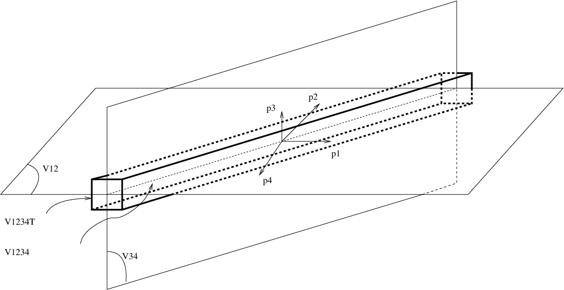
Refer to caption

Figure 2: Example of an intersection in dimension 33. 𝒯{1,2}τ{\mathcal{T}}^{\tau}_{\{1,2\}} is in between to planes, parallel to 𝒯{1,2}{{\mathcal{T}}_{\{1,2\}}}. Same remark for 𝒯{3,4}τ{\mathcal{T}}^{\tau}_{\{3,4\}}. The set 𝒯{1,2}τ∩𝒯{3,4}τ{\mathcal{T}}^{\tau}_{\{1,2\}}\cap{\mathcal{T}}^{\tau}_{\{3,4\}} is of the form W+PW⊥​ℒg~​(τ)W+P_{W^{\bot}}{\mathcal{L}}_{\tilde{g}}(\tau), where g~\tilde{g} is a norm and for W=𝒯{1,2}∩𝒯{3,4}W={{\mathcal{T}}_{\{1,2\}}}\cap{{\mathcal{T}}_{\{3,4\}}}. We also have dim(𝒯{1,2}∩𝒯{3,4})<d​i​m​(𝒯{1,2})=d​i​m​(𝒯{3,4})\dim({{\mathcal{T}}_{\{1,2\}}}\cap{{\mathcal{T}}_{\{3,4\}}})<dim({{\mathcal{T}}_{\{1,2\}}})=dim({{\mathcal{T}}_{\{3,4\}}}).

This section is devoted to prove quite an intuitive result on the estimate of the intersection of two sets 𝒯Jτ{\mathcal{T}}^{\tau}_{J}. It uses all notations introduced in §2.2 and is illustrated on Figure 2.

Proposition 2

Let J1⊂IJ_{1}\subset I and J2⊂IJ_{2}\subset I be such that 𝒯J1≠𝒯J2{{\mathcal{T}}_{J_{1}}}\neq{{\mathcal{T}}_{J_{2}}} and dim(𝒯J1)=dim(𝒯J2)=defK\dim({{\mathcal{T}}_{J_{1}}})=\dim({{\mathcal{T}}_{J_{2}}})\stackrel{{\scriptstyle\rm def}}{{=}}K. Let τ>0\tau>0 and θ>0\theta>0. Then the set given below

𝒯J1τ∩𝒯J2τ∩ℒfd​(θ){\mathcal{T}}^{\tau}_{J_{1}}\cap{\mathcal{T}}^{\tau}_{J_{2}}\cap{\mathcal{L}}_{f_{d}}(\theta) (26)

is closed and measurable. Moreover, there is a constant  δJ1,J2∈[0,3​Δ¯]\delta_{\!J_{1}\!,\!J_{2}}\in[0,3{\overline{\Delta}}] (where Δ¯{\overline{\Delta}} is given in Lemma 1(iii)) such that for θ≥δJ1,J2​τ\theta\geq\delta_{\!J_{1}\!,\!J_{2}}\tau we have

𝕃N(𝒯J1τ∩𝒯J2τ∩ℒfd(θ))≤QJ1,J2τN−k(θ+δJ1,J2τ)k,k=dim(𝒯J1∩𝒯J2),{\mathbb{L}}^{{}^{{}_{\!\!N}}}\big({\mathcal{T}}^{\tau}_{J_{1}}\cap{\mathcal{T}}^{\tau}_{J_{2}}\cap{\mathcal{L}}_{f_{d}}(\theta)\big)\leq Q_{\!J_{1}\!,\!J_{2}}\tau^{N-k}(\theta+\delta_{\!J_{1}\!,\!J_{2}}\tau)^{k},~~~~k=\dim\big({{\mathcal{T}}_{J_{1}}}\cap{{\mathcal{T}}_{J_{2}}}\big),

where the constant QJ1,J2Q_{\!J_{1}\!,\!J_{2}} reads

QJ1,J2=def𝕃N−k(W⊥∩ℒ∥.∥2(2δ2))𝕃k(W∩ℒfd(1))forW=def𝒯J1∩𝒯J2.Q_{\!J_{1}\!,\!J_{2}}\stackrel{{\scriptstyle\rm def}}{{=}}{\mathbb{L}}^{{}^{{}_{\!\!N-k}}}\big(W^{\bot}\cap{\mathcal{L}}_{\|.\|_{2}}(2\delta_{2})\big)~{\mathbb{L}}^{{}^{{}_{\!\!k}}}\big(W\cap{\mathcal{L}}_{f_{d}}(1)\big)~~~~\mbox{for}~~~W\stackrel{{\scriptstyle\rm def}}{{=}}{{\mathcal{T}}_{J_{1}}}\cap{{\mathcal{T}}_{J_{2}}}. (27)

Notice that QJ1,J2Q_{\!J_{1}\!,\!J_{2}} depends only on (ψj)j∈J1(\psi_{j})_{j\in J_{1}} and (ψj)j∈J2(\psi_{j})_{j\in J_{2}}, and the norms ∥.∥\|.\| and fdf_{d}. A tighter bound can be found in the proof of the proposition (see equation (37)). The bound is expressed in terms of a norm g~\tilde{g} constructed there.

Remark 5

Since k=dimW≤K−1k=\dim W\leq K-1, we have the following asymptotical result:

𝕃N(𝒯J1τ∩𝒯J2τ∩ℒfd(θ))\displaystyle{\mathbb{L}}^{{}^{{}_{\!\!N}}}\big({\mathcal{T}}^{\tau}_{J_{1}}\cap{\mathcal{T}}^{\tau}_{J_{2}}\cap{\mathcal{L}}_{f_{d}}(\theta)\big) ≤\displaystyle\leq QJ1,J2​θN​(τθ)N−k​(1+δJ1,J2​τθ)k\displaystyle Q_{\!J_{1}\!,\!J_{2}}~\theta^{N}\left(\frac{\tau}{\theta}\right)^{N-k}\left(1+\delta_{\!J_{1},J_{2}}\frac{\tau}{\theta}\right)^{k}
=\displaystyle= QJ1,J2​θN​(τθ)N−k+o⁡((τθ)N−k)as​τθ→0\displaystyle Q_{\!J_{1}\!,\!J_{2}}~\theta^{N}\left(\frac{\tau}{\theta}\right)^{N-k}+o\left(\left(\frac{\tau}{\theta}\right)^{N-k}\right)~~~~\mbox{as}~~\frac{\tau}{\theta}\to 0
=\displaystyle= θN​o​((τθ)N−K)as​τθ→0.\displaystyle\theta^{N}o\left(\left(\frac{\tau}{\theta}\right)^{N-K}\right)~~~~~~~~~~~~~~~~~~~~~~~~~\mbox{as}~~\frac{\tau}{\theta}\to 0.

Proof. The subset in (26) is closed and measurable, as being a finite intersection of closed measurable sets.

Let

h1:𝒯J1⊥→ℝandh2:𝒯J2⊥→ℝh_{1}:{\mathcal{T}}^{\bot}_{J_{1}}\to\mathbb{R}~~~~\mbox{and}~~~~h_{2}:{\mathcal{T}}^{\bot}_{J_{2}}\to\mathbb{R}

be the norms exhibited in Lemma 1—see equation (8)—such that for any τ≥0\tau\geq 0,

ℒh1(τ)=P𝒯J1⊥(ℒ∥.∥(τ))andℒh2(τ)=P𝒯J2⊥(ℒ∥.∥(τ)).{\mathcal{L}}_{h_{1}}(\tau)=P_{{{\mathcal{T}}_{J_{1}^{\bot}}}}\left({\mathcal{L}}_{\|.\|}(\tau)\right)~~~~\mbox{and}~~~~{\mathcal{L}}_{h_{2}}(\tau)=P_{{{\mathcal{T}}_{J_{2}^{\bot}}}}\left({\mathcal{L}}_{\|.\|}(\tau)\right).

Reminding that by definition

W=𝒯J1∩𝒯J2,W={{\mathcal{T}}_{J_{1}}}\cap{{\mathcal{T}}_{J_{2}}},

De Morgan’s law shows that

W⊥=𝒯J1⊥+𝒯J2⊥.W^{\bot}={\mathcal{T}}^{\bot}_{J_{1}}+{\mathcal{T}}^{\bot}_{J_{2}}.

Below we express the latter sum as a direct sum of subspaces:

W⊥=(𝒯J1⊥∩𝒯J2⊥)\displaystyle W^{\bot}=\big({\mathcal{T}}^{\bot}_{J_{1}}\cap{\mathcal{T}}^{\bot}_{J_{2}}\big) ⊕\displaystyle\oplus (𝒯J1⊥∩𝒯J2)\displaystyle\Big({\mathcal{T}}^{\bot}_{J_{1}}\cap{{\mathcal{T}}_{J_{2}}}\Big) (28)
⊕\displaystyle\oplus (𝒯J1∩𝒯J2⊥).\displaystyle\Big(\;{{\mathcal{T}}_{J_{1}}}\;\cap{\mathcal{T}}^{\bot}_{J_{2}}\Big).

Notice that we have

𝒯J1⊥=(𝒯J1⊥∩𝒯J2⊥)⊕(𝒯J1⊥∩𝒯J2),𝒯J2⊥=(𝒯J1⊥∩𝒯J2⊥)⊕(𝒯J1∩𝒯J2⊥),\begin{array}[]{l}{\mathcal{T}}^{\bot}_{J_{1}}=\big({\mathcal{T}}^{\bot}_{J_{1}}\cap{\mathcal{T}}^{\bot}_{J_{2}}\big)\oplus\Big({\mathcal{T}}^{\bot}_{J_{1}}\cap{{\mathcal{T}}_{J_{2}}}\Big),\\ \\ {\mathcal{T}}^{\bot}_{J_{2}}=\big({\mathcal{T}}^{\bot}_{J_{1}}\cap{\mathcal{T}}^{\bot}_{J_{2}}\big)\oplus\Big({{\mathcal{T}}_{J_{1}}}\cap{\mathcal{T}}^{\bot}_{J_{2}}\Big),\end{array} (29)

as well as

𝒯J1=W⊕(𝒯J1∩𝒯J2⊥),𝒯J2=W⊕(𝒯J1⊥∩𝒯J2).\begin{array}[]{l}{{\mathcal{T}}_{J_{1}}}=W\oplus\Big({{\mathcal{T}}_{J_{1}}}\cap{\mathcal{T}}^{\bot}_{J_{2}}\Big),\\ \\ {{\mathcal{T}}_{J_{2}}}=W\oplus\Big({\mathcal{T}}^{\bot}_{J_{1}}\cap{{\mathcal{T}}_{J_{2}}}\Big).\end{array} (30)

¿From (28), any u∈W⊥u\in W^{\bot} has a unique decomposition as

u=u1+u2+u3whereu1∈𝒯J1⊥∩𝒯J2⊥u2∈𝒯J1⊥∩𝒯J2u3∈𝒯J1∩𝒯J2⊥u=u_{1}+u_{2}+u_{3}~~~~~~\mbox{where}~~~~~~\begin{array}[]{l}u_{1}\in{\mathcal{T}}^{\bot}_{J_{1}}\cap{\mathcal{T}}^{\bot}_{J_{2}}\\ u_{2}\in{\mathcal{T}}^{\bot}_{J_{1}}\cap{{\mathcal{T}}_{J_{2}}}\\ u_{3}\in{{\mathcal{T}}_{J_{1}}}~\cap{\mathcal{T}}^{\bot}_{J_{2}}\end{array} (31)

Using these notations, we introduce the following function:

g:W⊥\displaystyle g:W^{\bot} →\displaystyle\to ℝ\displaystyle\mathbb{R}
u\displaystyle u →\displaystyle\to g⁡(u)=sup{h1​(u1+u2),h2​(u1+u3)}.\displaystyle g(u)=\sup\big\{h_{1}(u_{1}+u_{2}),h_{2}(u_{1}+u_{3})\big\}. (32)

In the next lines we show that gg is a norm on W⊥W^{\bot}:

  • •

    h1h_{1} and h2h_{2} being norms, g⁡(λ​u)=|λ|​g​(u)g(\lambda u)=|\lambda|g(u), for all λ∈ℝ\lambda\in\mathbb{R};

  • •

    if g⁡(u)=0g(u)=0 then u1+u2=u1+u3=0u_{1}+u_{2}=u_{1}+u_{3}=0; noticing that u1⊥u2u_{1}\bot u_{2} and that u1⊥u3u_{1}\bot u_{3} yields u=0u=0;

  • •

    for u∈W⊥u\in W^{\bot} and v∈W⊥v\in W^{\bot} (both decomposed according to (31)),

    g⁡(u+v)\displaystyle g(u+v) =\displaystyle= sup{h1​(u1+u2+v1+v2),h2​(u1+u3+v1+v3)}\displaystyle\sup\big\{h_{1}(u_{1}+u_{2}+v_{1}+v_{2}),h_{2}(u_{1}+u_{3}+v_{1}+v_{3})\big\}
    ≤\displaystyle\leq sup{h1​(u1+u2)+h1​(v1+v2),h2​(u1+u3)+h2​(v1+v3)}\displaystyle\sup\big\{h_{1}(u_{1}+u_{2})+h_{1}(v_{1}+v_{2}),h_{2}(u_{1}+u_{3})+h_{2}(v_{1}+v_{3})\big\}
    ≤\displaystyle\leq sup{h1​(u1+u2),h2​(u1+u3)}+sup{h1​(v1+v2),h2​(v1+v3)}\displaystyle\sup\big\{h_{1}(u_{1}+u_{2}),h_{2}(u_{1}+u_{3})\big\}+\sup\big\{h_{1}(v_{1}+v_{2}),h_{2}(v_{1}+v_{3})\big\}
    =\displaystyle= g⁡(u)+g⁡(v).\displaystyle g(u)+g(v).

Furthermore, gg can be extended to a norm g~\tilde{g} on ℝN\mathbb{R}^{N} such that ∀u∈W⊥\forall u\in W^{\bot}, we have g~​(u)=g​(u)\tilde{g}(u)=g(u) and

ℒg​(τ)=PW⊥​(ℒg~​(τ)),∀τ>0.{\mathcal{L}}_{g}(\tau)=P_{W^{\bot}}\left({\mathcal{L}}_{\tilde{g}}(\tau)\right),~~~~\forall\tau>0. (33)

Let us then define

Wτ\displaystyle W^{\tau} =\displaystyle= W+PW⊥​(ℒg~​(τ))\displaystyle W+P_{W^{\bot}}\left({\mathcal{L}}_{\tilde{g}}(\tau)\right) (34)
=\displaystyle= {w+u:(u,w)∈(W⊥×W),g(u)≤τ}.\displaystyle\Big\{w+u:(u,w)\in(W^{\bot}\!\!\times W),~g(u)\leq\tau\Big\}.

We are going to show that (𝒯J1τ∩𝒯J2τ)⊂Wτ\left({\mathcal{T}}^{\tau}_{J_{1}}\cap{\mathcal{T}}^{\tau}_{J_{2}}\right)\subset W^{\tau}. In order to do so, we consider an arbitrary

v∈𝒯J1τ∩𝒯J2τ.v\in{\mathcal{T}}^{\tau}_{J_{1}}\cap{\mathcal{T}}^{\tau}_{J_{2}}. (35)

It admits a unique decomposition of the form

v=w+u1+u2+u3,v=w+u_{1}+u_{2}+u_{3},

where w∈Ww\in W, and u1,u2u_{1},~u_{2} and u3u_{3} are decomposed according to (31). The latter, combined with (29) and (30) shows that

u1+u2∈𝒯J1⊥\displaystyle u_{1}+u_{2}\in{\mathcal{T}}^{\bot}_{J_{1}}   and   w+u3∈𝒯J1,\displaystyle w+u_{3}\in{{\mathcal{T}}_{J_{1}}},
u1+u3∈𝒯J2⊥\displaystyle u_{1}+u_{3}\in{\mathcal{T}}^{\bot}_{J_{2}}   and   w+u2∈𝒯J2.\displaystyle w+u_{2}\in{{\mathcal{T}}_{J_{2}}}.

The inclusions given above, combined with (35), show that

h1​(u1+u2)≤τandh2​(u1+u3)≤τ.h_{1}(u_{1}+u_{2})\leq\tau~~~~~\mbox{and}~~~~~h_{2}(u_{1}+u_{3})\leq\tau.

By the definition of gg in (31)-(32), the inequalities given above imply that g⁡(u)≤τg(u)\leq\tau. Combining this with the definition of WτW^{\tau} in (34) entails that v∈Wτv\in W^{\tau}. Consequently,

(𝒯J1τ∩𝒯J2τ)⊂Wτand(𝒯J1τ∩𝒯J2τ∩ℒfd​(θ))⊂(Wτ∩ℒfd​(θ)).\Big({\mathcal{T}}^{\tau}_{J_{1}}\cap{\mathcal{T}}^{\tau}_{J_{2}}\Big)\subset W^{\tau}~~~~\mbox{and}~~~~\Big({\mathcal{T}}^{\tau}_{J_{1}}\cap{\mathcal{T}}^{\tau}_{J_{2}}\cap{\mathcal{L}}_{f_{d}}(\theta)\Big)~\subset~\Big(W^{\tau}\cap{\mathcal{L}}_{f_{d}}(\theta)\Big).

It follows that

𝕃N(𝒯J1τ∩𝒯J2τ∩ℒfd(θ))≤𝕃N(Wτ∩ℒfd(θ)).{\mathbb{L}}^{{}^{{}_{\!\!N}}}\big({\mathcal{T}}^{\tau}_{J_{1}}\cap{\mathcal{T}}^{\tau}_{J_{2}}\cap{\mathcal{L}}_{f_{d}}(\theta)\big)\leq{\mathbb{L}}^{{}^{{}_{\!\!N}}}\big(W^{\tau}\cap{\mathcal{L}}_{f_{d}}(\theta)\big).

Applying now the right-hand side of (18) in Proposition 1 with WτW^{\tau} in place of VτV^{\tau} and taking δJ1,J2\delta_{\!J_{1}\!,\!J_{2}} such that

fd​(u)≤δJ1,J2​g​(u),∀u∈W⊥,f_{d}(u)\leq\delta_{\!J_{1}\!,\!J_{2}}g(u),~~~\forall u\in W^{\bot}, (36)

leads to

𝕃N(Wτ∩ℒfd(θ))≤QJ1,J2′τN−k(θ+δJ1,J2τ)k,{\mathbb{L}}^{{}^{{}_{\!\!N}}}\big(W^{\tau}\cap{\mathcal{L}}_{f_{d}}(\theta)\big)\leq Q^{\prime}_{\!J_{1}\!,\!J_{2}}\tau^{N-k}(\theta+\delta_{\!J_{1}\!,\!J_{2}}\tau)^{k},

where it is easy to see that

QJ1,J2′=𝕃N−k(PW⊥(ℒg~(τ)))𝕃k(W∩ℒfd(1))=𝕃N−k(ℒg(1))𝕃k(W∩ℒfd(1)).Q^{\prime}_{\!J_{1}\!,\!J_{2}}={\mathbb{L}}^{{}^{{}_{\!\!N-k}}}\big(P_{W^{\bot}}\left({\mathcal{L}}_{\tilde{g}}(\tau)\right)\big){\mathbb{L}}^{{}^{{}_{\!\!k}}}\big(W\cap{\mathcal{L}}_{f_{d}}(1)\big)={\mathbb{L}}^{{}^{{}_{\!\!N-k}}}\big({\mathcal{L}}_{g}(1)\big){\mathbb{L}}^{{}^{{}_{\!\!k}}}\big(W\cap{\mathcal{L}}_{f_{d}}(1)\big). (37)

In order to obtain (27), we are going to show that ℒg(1)⊂(ℒ∥.∥2(2δ2)∩W⊥){\mathcal{L}}_{g}(1)\subset\left({\mathcal{L}}_{\|.\|_{2}}(2\delta_{2})\cap W^{\bot}\right). Using Lemma 1 (ii), if u∈W⊥u\in W^{\bot} is decomposed according to (31), we obtain

‖u‖2=(‖u1‖22+‖u2‖22+‖u3‖22)12\displaystyle\|u\|_{2}=\left(\|u_{1}\|_{2}^{2}+\|u_{2}\|_{2}^{2}+\|u_{3}\|_{2}^{2}\right)^{\frac{1}{2}} ≤\displaystyle\leq ‖2​u1+u2+u3‖2\displaystyle\|2u_{1}+u_{2}+u_{3}\|_{2}
≤\displaystyle\leq ‖u1+u2‖2+‖u1+u3‖2\displaystyle\|u_{1}+u_{2}\|_{2}+\|u_{1}+u_{3}\|_{2}
≤\displaystyle\leq δ2​h1​(u1+u2)+δ2​h2​(u1+u3)\displaystyle\delta_{2}h_{1}(u_{1}+u_{2})+\delta_{2}h_{2}(u_{1}+u_{3})
≤\displaystyle\leq 2​δ2​g​(u).\displaystyle 2\delta_{2}g(u).

So ℒg(1)⊂(ℒ∥.∥2(2δ2)∩W⊥){\mathcal{L}}_{g}(1)\subset\left({\mathcal{L}}_{\|.\|_{2}}(2\delta_{2})\cap W^{\bot}\right) and QJ1,J2′≤QJ1,J2Q^{\prime}_{\!J_{1}\!,\!J_{2}}\leq Q_{\!J_{1}\!,\!J_{2}}, for QJ1,J2Q_{\!J_{1}\!,\!J_{2}} as given in the proposition.

At last, we need to build a uniform bound on δJ1,J2\delta_{\!J_{1}\!,\!J_{2}} giving rise to (36). Using Lemma 1 (ii), if u∈W⊥u\in W^{\bot} is decomposed according to (31), we obtain

fd​(u)=fd​(u1+u2+u3)\displaystyle f_{d}(u)=f_{d}(u_{1}+u_{2}+u_{3}) ≤\displaystyle\leq fd​(2​u1+u2+u3)+fd​(u1)\displaystyle f_{d}(2u_{1}+u_{2}+u_{3})+f_{d}(u_{1}) (38)
≤\displaystyle\leq fd​(u1+u2)+fd​(u1+u3)+fd​(u1)\displaystyle f_{d}(u_{1}+u_{2})+f_{d}(u_{1}+u_{3})+f_{d}(u_{1})
≤\displaystyle\leq Δ¯​h1​(u1+u2)+Δ¯​h2​(u1+u3)+δ1​‖u1‖2.\displaystyle{\overline{\Delta}}h_{1}(u_{1}+u_{2})+{\overline{\Delta}}h_{2}(u_{1}+u_{3})+\delta_{1}\|u_{1}\|_{2}.

Using (13), ‖u1‖2\|u_{1}\|_{2} satisfies the following two inequalities

‖u1‖2\displaystyle\|u_{1}\|_{2} ≤\displaystyle\leq ‖u1+u2‖2≤δ2​h1​(u1+u2),\displaystyle\|u_{1}+u_{2}\|_{2}\leq\delta_{2}h_{1}(u_{1}+u_{2}),
‖u1‖2\displaystyle\|u_{1}\|_{2} ≤\displaystyle\leq ‖u1+u3‖2≤δ2​h2​(u1+u3).\displaystyle\|u_{1}+u_{3}\|_{2}\leq\delta_{2}h_{2}(u_{1}+u_{3}).

Adding these inequalities, we obtain

δ1​‖u1‖2≤Δ¯2​(h1​(u1+u2)+h2​(u1+u3)).\delta_{1}\|u_{1}\|_{2}\leq\frac{{\overline{\Delta}}}{2}~\big(h_{1}(u_{1}+u_{2})+h_{2}(u_{1}+u_{3})\big).

Using (38), we finally conclude that, for u∈W⊥u\in W^{\bot}

fd​(u)\displaystyle f_{d}(u) ≤\displaystyle\leq 3​Δ¯2​(h1​(u1+u2)+h2​(u1+u3))\displaystyle\frac{3{\overline{\Delta}}}{2}~\big(h_{1}(u_{1}+u_{2})+h_{2}(u_{1}+u_{3})\big)
≤\displaystyle\leq 3​Δ¯​g​(u).\displaystyle 3{\overline{\Delta}}~g(u).

The proof is complete. □\Box

4 Sets of data yielding KK-sparse solutions or sparser

For any given K∈{0,…,N}K\in\{0,\ldots,N\} and τ>0\tau>0, we introduce the subset ℐτ​(K){{\mathcal{I}}^{\tau}\left(K\right)} as it follows:

ℐτ​(K)=def{d∈ℝN:val⁡(𝒫d)≤K}.\displaystyle{{\mathcal{I}}^{\tau}\left(K\right)}\stackrel{{\scriptstyle\rm def}}{{=}}\big\{d\in\mathbb{R}^{N}~:~\val({\mathcal{P}}_{d})\leq K\big\}. (39)

All data belonging to ℐτ​(K){{\mathcal{I}}^{\tau}\left(K\right)} generate a solution of (𝒫d)({\mathcal{P}}_{d})—see (2)—which involves at most KK non-zero components.

Let us define

GK=def{J⊂I:dim(𝒯J)≤K},G_{K}\stackrel{{\scriptstyle\rm def}}{{=}}\big\{J\subset I:\dim({{\mathcal{T}}_{J}})\leq K\big\}, (40)

and remind that 𝒯J=span⁡((ψj)j∈J){{\mathcal{T}}_{J}}=\Span\left((\psi_{j})_{j\in J}\right) according to (22).

The next proposition states a strong and slightly surprising result.

Proposition 3

For any K∈{0,…,N}K\in\{0,\ldots,N\}, any norm ∥.∥\|.\| and any τ>0\tau>0, we have

ℐτ(K)=⋃J∈GK𝒯J+ℒ∥.∥(τ).{{\mathcal{I}}^{\tau}\left(K\right)}=\bigcup_{J\in G_{K}}{{\mathcal{T}}_{J}}+{\mathcal{L}}_{\|.\|}(\tau).

Some sets ℐτ​(K){{\mathcal{I}}^{\tau}\left(K\right)}, as defined in (39) and explained in the last proposition, are illustrated on Figure 1.

Proof. The case K=0K=0 is trivial (G0={∅}G_{0}=\{\emptyset\}) and we assume in the following that K≥1K\geq 1.

Let d∈ℐτ​(K)d\in{{\mathcal{I}}^{\tau}\left(K\right)}. This means there is (λi)i∈I(\lambda_{i})_{i\in I}—a solution of (𝒫d)({\mathcal{P}}_{d})—that satisfies ℓ0​((λi)i∈I)≤K\ell_{0}((\lambda_{i})_{i\in I})\leq K. Hence

d=∑i∈Jλi​ψi+w\displaystyle d=\sum_{i\in J}\lambda_{i}\psi_{i}+w~ withw∈ℒ∥.∥(τ)\displaystyle\mbox{with}~~~w\in{\mathcal{L}}_{\|.\|}(\tau)
and​J={i∈I:λi≠0}​with​#​J≤K.\displaystyle\mbox{and}~~~J=\{i\in I:\lambda_{i}\neq 0\}~~~\mbox{with}~~~\#J\leq K.

Consequently dim(𝒯J)≤#​J≤K\dim({{\mathcal{T}}_{J}})\leq\#J\leq K, which implies that d∈∪J∈GK𝒯J+ℒ∥.∥(τ)d\in\cup_{J\in G_{K}}{{\mathcal{T}}_{J}}+{\mathcal{L}}_{\|.\|}(\tau).

Conversely, let d∈∪J∈GK𝒯J+ℒ∥.∥(τ)d\in\cup_{J\in G_{K}}{{\mathcal{T}}_{J}}+{\mathcal{L}}_{\|.\|}(\tau), then d=v+wd=v+w where v∈∪J∈GK𝒯Jv\in\cup_{J\in G_{K}}{{\mathcal{T}}_{J}} and w∈ℒ∥.∥(τ)w\in{\mathcal{L}}_{\|.\|}(\tau). Then:

  • •

    ∃J⊂I\exists~J\subset I such that v∈𝒯Jv\in{{\mathcal{T}}_{J}} and the latter satisfies dim(𝒯J)≤K\dim({{\mathcal{T}}_{J}})\leq K;

  • •

    there are real numbers (λi)i∈J(\lambda_{i})_{i\in J} involving at most dim(𝒯J)\dim({{\mathcal{T}}_{J}}) non-zero components (hence ℓ0​((λi)i∈J)≤dim(𝒯J)≤K\ell_{0}((\lambda_{i})_{i\in J})\leq\dim({{\mathcal{T}}_{J}})\leq K) such that v=∑i∈Jλi​ψiv=\sum_{i\in J}\lambda_{i}\psi_{i}.

  • •

    w∈ℒ∥.∥(τ)w\in{\mathcal{L}}_{\|.\|}(\tau) means that ‖w‖≤τ\|w\|\leq\tau.

It follows that  d=∑i∈Jλi​ψi+w∈ℐτ​(K)d=\sum_{i\in J}\lambda_{i}\psi_{i}+w~\in{{\mathcal{I}}^{\tau}\left(K\right)}. □\Box

Given J⊂IJ\subset I, remind that 𝒯J=span⁡((ψj)j∈J){{\mathcal{T}}_{J}}=\Span\left((\psi_{j})_{j\in J}\right)—see (22). Since (ψi)i∈I(\psi_{i})_{i\in I} is a general family of vectors, there may be numerous subsets JnJ_{n}, n=1,2,…n=1,2,\ldots, such that 𝒯Jn=𝒯Jm{{\mathcal{T}}_{J_{n}}}={{\mathcal{T}}_{J_{m}}} and Jn≠JmJ_{n}\neq J_{m}. A non-redundant listing of all possible subspaces 𝒯J{{\mathcal{T}}_{J}} when JJ runs over all subsets of II can be obtained with the help of the notations below.

For any K=0,…,NK=0,\ldots,N, define 𝒥⁡(K){\mathcal{J}}(K) by the following three properties:

{(a)𝒥⁡(K)⊂{J⊂I:dim(𝒯J)=K};(b)J1,J2∈𝒥⁡(K)​and​J1≠J2⟹𝒯J1≠𝒯J2;(c)𝒥(K)is maximal:if ​J1⊂I​yields​dim(𝒯J1)=K​then​∃J∈𝒥⁡(K)​such that​𝒯J=𝒯J1.\left\{\begin{array}[]{lll}(a)&&{\mathcal{J}}(K)\subset\big\{J\subset I:\dim({{\mathcal{T}}_{J}})=K\big\};\\ \\ (b)&&J_{1},J_{2}\in{\mathcal{J}}(K)~~\mbox{and}~~J_{1}\neq J_{2}~~\Longrightarrow~~{{\mathcal{T}}_{J_{1}}}\neq{{\mathcal{T}}_{J_{2}}};\\ \\ (c)&&{\mathcal{J}}(K)~\mbox{is maximal:}\\ &&\mbox{if~~}J_{1}\subset I~~\mbox{yields}~~\dim({{\mathcal{T}}_{J_{1}}})=K~~\mbox{then}~~\exists J\in{\mathcal{J}}(K)~~\mbox{such that}~~{{\mathcal{T}}_{J}}={{\mathcal{T}}_{J_{1}}}.\end{array}\right. (41)

Notice that in particular, 𝒥⁡(0)={∅}{\mathcal{J}}(0)=\{\emptyset\} and #​𝒥​(N)=1\#{\mathcal{J}}(N)=1. One can observe that GKG_{K}, as defined in (40), satisfies

GK⊃⋃k=0K𝒥⁡(k)G_{K}\supset\bigcup_{k=0}^{K}{\mathcal{J}}(k)

and

{𝒯J:J∈GK}={𝒯J:J∈𝒥⁡(k)​ for ​k∈{0,…,K}}.\{{{\mathcal{T}}_{J}}:J\in G_{K}\}=\{{{\mathcal{T}}_{J}}:J\in{\mathcal{J}}(k)\mbox{ for }k\in\{0,\ldots,K\}\}. (42)

Using these notations, we can give a more convenient formulation of Proposition 3.

Theorem 1

For any K∈{0,…,N}K\in\{0,\ldots,N\}, any norm ∥.∥\|.\| and any τ>0\tau>0, we have

ℐτ​(K)=⋃J∈𝒥⁡(K)𝒯Jτ,{{\mathcal{I}}^{\tau}\left(K\right)}=\bigcup_{J\in{\mathcal{J}}(K)}{\mathcal{T}}^{\tau}_{J},

where we remind that for any J⊂IJ\subset I and τ>0\tau>0, 𝒯Jτ{\mathcal{T}}^{\tau}_{J} is defined by (23), and 𝒥⁡(K){\mathcal{J}}(K) is defined by (41).

As a consequence, ℐτ​(K){{\mathcal{I}}^{\tau}\left(K\right)} is closed and measurable.

Proof. The case J=∅J=\emptyset (and K=0K=0) is trivial because of the convention span⁡(∅)={0}\Span(\emptyset)=\{0\} and 𝒥⁡(0)={∅}{\mathcal{J}}(0)=\{\emptyset\}.

Let us first prove that ℐτ​(K)=⋃J∈GK𝒯Jτ{{\mathcal{I}}^{\tau}\left(K\right)}=\bigcup_{J\in G_{K}}{\mathcal{T}}^{\tau}_{J}. Using Proposition 3,

ℐτ(K)=(⋃J∈GK𝒯J)+ℒ∥.∥(τ)=⋃J∈GK(𝒯J+ℒ∥.∥(τ)).{{\mathcal{I}}^{\tau}\left(K\right)}=\left(\bigcup_{J\in G_{K}}{{\mathcal{T}}_{J}}\right)+{\mathcal{L}}_{\|.\|}(\tau)=\bigcup_{J\in G_{K}}\big({{\mathcal{T}}_{J}}+{\mathcal{L}}_{\|.\|}(\tau)\big).

The last equality above is a trivial observation. Using Lemma 2, this summarizes us

ℐτ​(K)=⋃J∈GK𝒯Jτ.{{\mathcal{I}}^{\tau}\left(K\right)}=\bigcup_{J\in G_{K}}{\mathcal{T}}^{\tau}_{J}.

Using (42), we deduce that

{𝒯Jτ:J∈GK}={𝒯Jτ:J∈𝒥⁡(k)​ for ​k∈{0,…,K}},\{{\mathcal{T}}^{\tau}_{J}:J\in G_{K}\}=\big\{{\mathcal{T}}^{\tau}_{J}:J\in{\mathcal{J}}(k)\mbox{ for }k\in\{0,\ldots,K\}\big\},

and therefore,

ℐτ​(K)=⋃k=0K⋃J∈𝒥⁡(k)𝒯Jτ.{{\mathcal{I}}^{\tau}\left(K\right)}=\bigcup_{k=0}^{K}\bigcup_{J\in{\mathcal{J}}(k)}{\mathcal{T}}^{\tau}_{J}.

Moreover, for any k<Kk<K and J∈𝒥⁡(k)J\in{\mathcal{J}}(k), we can find J1∈𝒥⁡(K)J_{1}\in{\mathcal{J}}(K) such that 𝒯J⊂𝒯J1{{\mathcal{T}}_{J}}\subset{{\mathcal{T}}_{J_{1}}}. Using Lemma 2, we find that 𝒯Jτ⊂𝒯J1τ{\mathcal{T}}^{\tau}_{J}\subset{\mathcal{T}}^{\tau}_{J_{1}}. Consequently,

ℐτ​(K)=⋃J∈𝒥⁡(K)𝒯Jτ.{{\mathcal{I}}^{\tau}\left(K\right)}=\bigcup_{J\in{\mathcal{J}}(K)}{\mathcal{T}}^{\tau}_{J}.

This completes the proof of the first statement.

By Proposition 1, ℐτ​(K){{\mathcal{I}}^{\tau}\left(K\right)} is a finite union of closed measurable sets, hence it is closed and measurable as well. □\Box

For any K=0,…,NK=0,\ldots,N, define the constants δ^K\hat{\delta}_{K} and 𝑪¯\overline{C}K as it follows:

δ^K\displaystyle\hat{\delta}_{K} =def\displaystyle\stackrel{{\scriptstyle\rm def}}{{=}} maxJ∈𝒥⁡(K)⁡δJ,\displaystyle\max_{J\in{\mathcal{J}}(K)}\delta_{J}, (43)
𝑪¯\overline{C}K =def\displaystyle\stackrel{{\scriptstyle\rm def}}{{=}} ∑J∈𝒥⁡(K)CJ,\displaystyle\sum_{J\in{\mathcal{J}}(K)}C_{J}, (44)

where δJ∈[0,Δ¯]\delta_{J}\in[0,{\overline{\Delta}}] and CJC_{J} are the constants exhibited in Corollary 1, assertion (ii). Clearly,

0≤δ^K≤Δ¯.0\leq\hat{\delta}_{K}\leq{\overline{\Delta}}. (45)

In particular,

𝑪¯0=𝕃N(ℒ∥.∥(1)) and 𝑪¯N=𝕃N(ℒfd(1)).\mbox{\boldmath$\overline{C}$\unboldmath${}_{0}$}={\mathbb{L}}^{{}^{{}_{\!\!N}}}\big({\mathcal{L}}_{\|.\|}(1)\big)\mbox{ and }\mbox{\boldmath$\overline{C}$\unboldmath${}_{N}$}={\mathbb{L}}^{{}^{{}_{\!\!N}}}\big({\mathcal{L}}_{f_{d}}(1)\big). (46)

With 𝒥⁡(K){\mathcal{J}}(K), let us associate the family of subsets :

ℋ(K,k)=def{(J1,J2)∈𝒥(K)2such thatdim(𝒯J1∩𝒯J2)=k},{\mathcal{H}}(K,k)\stackrel{{\scriptstyle\rm def}}{{=}}\Big\{(J_{1},J_{2})\in{\mathcal{J}}(K)^{2}~~\mbox{such that}~~\dim({{\mathcal{T}}_{J_{1}}}\cap{{\mathcal{T}}_{J_{2}}})=k\Big\}, (47)

where K=1,2,…,NK=1,2,\ldots,N and k=0,1,…,K−1k=0,1,\ldots,K-1.

Notice that ℋ⁡(K,k){\mathcal{H}}(K,k) may be empty for some kk. Consider (J1,J2)∈𝒥​(K)2(J_{1},J_{2})\in{\mathcal{J}}(K)^{2} such that

𝒯J1+𝒯J2=(𝒯J1∩𝒯J2)⊕(𝒯J1∩𝒯J2⊥)⊕(𝒯J2∩𝒯J1⊥)\displaystyle{{\mathcal{T}}_{J_{1}}}+{{\mathcal{T}}_{J_{2}}}=({{\mathcal{T}}_{J_{1}}}\cap{{\mathcal{T}}_{J_{2}}})\oplus({{\mathcal{T}}_{J_{1}}}\cap{{\mathcal{T}}_{J_{2}}}^{\bot})\oplus({{\mathcal{T}}_{J_{2}}}\cap{{\mathcal{T}}_{J_{1}}}^{\bot}) ⊂\displaystyle\subset ℝN\displaystyle\mathbb{R}^{N}
dim(𝒯J1+𝒯J2)=k+(K−k)+(K−k)\displaystyle\dim({{\mathcal{T}}_{J_{1}}}+{{\mathcal{T}}_{J_{2}}})=~~~~~~k~~~~~~+~~~(K-k)~~~+~~~(K-k)~~~ ≤\displaystyle\leq N\displaystyle N

and k≥2​K−Nk\geq 2K-N. We see that

ℋ⁡(K,k)≠∅⇒k≥2​K−N.{\mathcal{H}}(K,k)\neq\emptyset~~~~\Rightarrow~~~~k\geq 2K-N.

Conversely,

k<kK=defmax⁡{0,2​K−N}⇒ℋ⁡(K,k)=∅.k<k_{K}\stackrel{{\scriptstyle\rm def}}{{=}}\max\{0,~2K-N\}~~~~\Rightarrow~~~~{\mathcal{H}}(K,k)=\emptyset. (48)

Notice that ℋ⁡(N,k)=∅{\mathcal{H}}(N,k)=\emptyset, for all k=0,…,N−1k=0,\ldots,N-1 and that for any K=1,…,N−1K=1,\ldots,N-1, we have 0≤kK≤K−10\leq k_{K}\leq K-1.

For K∈{1,…,N−1}K\in\{1,\ldots,N-1\} and k∈{kK,…,K−1}k\in\{k_{K},\ldots,K-1\} let us define

δ^K,k′\displaystyle\hat{\delta}^{\prime}_{K,k} =def\displaystyle\stackrel{{\scriptstyle\rm def}}{{=}} max⁡{0,max(J1,J2)∈ℋ⁡(K,k)⁡δJ1,J2},\displaystyle{\displaystyle\max\left\{0,\max_{(J_{1},J_{2})\in{\mathcal{H}}(K,k)}\delta_{J_{1},J_{2}}\right\}}, (49)
𝑸¯\overline{Q}K,k =def\displaystyle\stackrel{{\scriptstyle\rm def}}{{=}} ∑(J1,J2)∈ℋ⁡(K,k)QJ1,J2\displaystyle\sum_{(J_{1},J_{2})\in{\mathcal{H}}(K,k)}Q_{\!J_{1}\!,\!J_{2}} (50)

where QJ1,J2Q_{\!J_{1}\!,\!J_{2}} and δJ1,J2∈[0,3​Δ¯]\delta_{J_{1},J_{2}}\in[0,3{\overline{\Delta}}] are as in Proposition 2. It is clear that if ℋ⁡(K,k)=∅{\mathcal{H}}(K,k)=\emptyset then we find 𝑸¯K,k=0\mbox{\boldmath$\overline{Q}$\unboldmath${}_{K,k}$}=0 and δ^K,k′=0\hat{\delta}^{\prime}_{K,k}=0. It follows that for any K=1,…,N−1K=1,\ldots,N-1 and any k=kK,…,K−1k=k_{K},\ldots,K-1

0≤δ^K,k′≤3​Δ¯.0\leq\hat{\delta}^{\prime}_{K,k}\leq 3{\overline{\Delta}}. (51)

Last, define

ΔK=def{δ^0, if ​K=0max⁡{ΔK−1,δ^K,maxkK≤k≤K−1⁡δ^K,k′}, if ​0<K<Nmax⁡{ΔN−1,δ^N}, if ​K=N\Delta_{K}\stackrel{{\scriptstyle\rm def}}{{=}}\left\{\begin{array}[]{ll}\hat{\delta}_{0}&\mbox{, if }K=0\\ {\displaystyle\max\left\{\Delta_{K-1},\hat{\delta}_{K},\max_{k_{K}\leq k\leq K-1}\hat{\delta}_{K,k}^{\prime}\right\}}&\mbox{, if }0<K<N\\ \max\big\{\Delta_{N-1},\hat{\delta}_{N}\big\}&\mbox{, if }K=N\\ \end{array}\right. (52)

Using (45) and (51),

0≤ΔK≤3​Δ¯.0\leq\Delta_{K}\leq 3{\overline{\Delta}}. (53)

All these constants, introduced between (43) and (52), depend only on the family (ψi)i∈I(\psi_{i})_{i\in I}, the norms ∥.∥\|.\| and fdf_{d}, KK and kk. Their upper bounds using Δ¯{\overline{\Delta}} only depend on ∥.∥\|.\| and fdf_{d}. They are involved in the theorem below which provides a critical result in this work.

Theorem 2

Let K∈{0,…,N}K\in\{0,\ldots,N\}, the norms ∥.∥\|.\| and fdf_{d}, and (ψi)i∈I(\psi_{i})_{i\in I}, be any. Let τ>0\tau>0 and θ≥τ​ΔK\theta\geq\tau\Delta_{K} where ΔK\Delta_{K} is defined in (52). The Lebesgue measure in ℝN\mathbb{R}^{N} of the set ℐτ​(K){{\mathcal{I}}^{\tau}\left(K\right)} defined by (39) satisfies

𝑪¯KτN−K(θ−δ^Kτ)K−θNε0(K,τ,θ)≤𝕃N(ℐτ(K)∩ℒfd(θ))≤𝑪¯KτN−K(θ+δ^Kτ)K,\mbox{\boldmath$\overline{C}$\unboldmath${}_{K}$}\tau^{N-K}(\theta-\hat{\delta}_{K}\tau)^{K}-\theta^{N}~\varepsilon_{0}(K,\tau,\theta)~\leq~{\mathbb{L}}^{{}^{{}_{\!\!N}}}\big({{\mathcal{I}}^{\tau}\left(K\right)}\cap{\mathcal{L}}_{f_{d}}(\theta)\big)~\leq~\mbox{\boldmath$\overline{C}$\unboldmath${}_{K}$}\tau^{N-K}(\theta+\hat{\delta}_{K}\tau)^{K}, (54)

where

ε0​(K,τ,θ)={0if ​K=0​ or ​K=N∑k=kKK−1𝑸¯K,k​(τθ)N−k​(1+δ^K,k′​τθ)kif ​0<K<N\varepsilon_{0}(K,\tau,\theta)=\left\{\begin{array}[]{ll}~~~~0&\mbox{\rm if }K=0\mbox{~~\rm or }K=N\\ {\displaystyle\sum_{k=k_{K}}^{K-1}\mbox{\boldmath$\overline{Q}$\unboldmath${}_{K,k}$}\left(\frac{\tau}{\theta}\right)^{N-k}\Big(1+\hat{\delta}_{K,k}^{\prime}\frac{\tau}{\theta}\Big)^{k}}&\mbox{\rm if }0<K<N\\ \end{array}\right. (55)

for 𝐂¯\overline{C}K, kKk_{K}, 𝐐¯\overline{Q}K,k, δ^k\hat{\delta}_{k} and δ^K,k′\hat{\delta}_{K,k}^{\prime} defined by (44), (48), (50), (43) and (49) respectively. Moreover, (45), (51) and (53) provide bounds on δ^K\hat{\delta}_{K}, δ^K,k′\hat{\delta}_{K,k}^{\prime} and ΔK\Delta_{K}, respectively, which depend only on ∥.∥\|.\| and fdf_{d}, via Δ¯{\overline{\Delta}} (see Lemma 1 (iii)).

Remark 6

We posit the assumptions of Theorem 2. Then asymptotically

𝕃N(ℐτ(K)∩ℒfd(θ))=𝑪¯KθN(τθ)N−K+θNo((τθ)N−K)asτθ→0.{\mathbb{L}}^{{}^{{}_{\!\!N}}}\big({{\mathcal{I}}^{\tau}\left(K\right)}\cap{\mathcal{L}}_{f_{d}}(\theta)\big)=\mbox{\boldmath$\overline{C}$\unboldmath${}_{K}$}~\theta^{N}\left(\frac{\tau}{\theta}\right)^{N-K}+\theta^{N}~o\left(\left(\frac{\tau}{\theta}\right)^{N-K}\right)~~\mbox{as}~~\frac{\tau}{\theta}\to 0.

Proof. Using Theorem 1, it is straightforward that

ℐτ​(K)∩ℒfd​(θ)=⋃J∈𝒥⁡(K)(𝒯Jτ∩ℒfd​(θ)){{\mathcal{I}}^{\tau}\left(K\right)}\cap{\mathcal{L}}_{f_{d}}(\theta)~=~\bigcup_{J\in{\mathcal{J}}(K)}\Big({\mathcal{T}}^{\tau}_{J}\cap{\mathcal{L}}_{f_{d}}(\theta)\Big) (56)

and that

𝕃N(ℐτ(K)∩ℒfd(θ))=𝕃N(⋃J∈𝒥⁡(K)(𝒯Jτ∩ℒfd(θ))).{\mathbb{L}}^{{}^{{}_{\!\!N}}}\big({{\mathcal{I}}^{\tau}\left(K\right)}\cap{\mathcal{L}}_{f_{d}}(\theta)\big)={\mathbb{L}}^{{}^{{}_{\!\!N}}}\big(\bigcup_{J\in{\mathcal{J}}(K)}\Big({\mathcal{T}}^{\tau}_{J}\cap{\mathcal{L}}_{f_{d}}(\theta)\Big)\big). (57)

When K=0K=0 or K=NK=N, we have #​𝒥​(K)=1\#{\mathcal{J}}(K)=1. Then, (54) is a straightforward consequence of (57) and Proposition 1 (the latter can be applied thanks to the assumption θ>τ​ΔK\theta>\tau\Delta_{K} and (52)).

The rest of the proof is to find relevant bounds for the right-hand side of (57) under the assumption that 0<K<N0<K<N.

Upper bound.

By the definition of a measure, and then using Corollary 1, it is found that

𝕃N(ℐτ(K)∩ℒfd(θ))\displaystyle{\mathbb{L}}^{{}^{{}_{\!\!N}}}\big({{\mathcal{I}}^{\tau}\left(K\right)}\cap{\mathcal{L}}_{f_{d}}(\theta)\big) ≤\displaystyle\leq ∑J∈𝒥⁡(K)𝕃N(𝒯Jτ∩ℒfd(θ))\displaystyle\sum_{J\in{\mathcal{J}}(K)}{\mathbb{L}}^{{}^{{}_{\!\!N}}}\big({\mathcal{T}}^{\tau}_{J}\cap{\mathcal{L}}_{f_{d}}(\theta)\big) (58)
≤\displaystyle\leq τN−K​∑J∈𝒥⁡(K)CJ​(θ+δJ​τ)K\displaystyle\tau^{N-K}\sum_{J\in{\mathcal{J}}(K)}C_{J}(\theta+\delta_{J}\tau)^{K}
≤\displaystyle\leq τN−K​(θ+δ^K​τ)K​∑J∈𝒥⁡(K)CJ\displaystyle\tau^{N-K}(\theta+\hat{\delta}_{K}\tau)^{K}\sum_{J\in{\mathcal{J}}(K)}C_{J}
=\displaystyle= 𝑪¯K​τN−K​(θ+δ^K​τ)K,\displaystyle\mbox{\boldmath$\overline{C}$\unboldmath${}_{K}$}~\tau^{N-K}(\theta+\hat{\delta}_{K}\tau)^{K},

where the constants δ^K\hat{\delta}_{K} and 𝑪¯\overline{C}K are defined in (43) and (44), respectively.

Lower bound.

First we represent the right-hand side of (56) as a union of disjoint subsets. Since 𝒥⁡(K){\mathcal{J}}(K) is finite, let us enumerate its elements as

𝒥⁡(K)={J1,…,JM}​where​M=#⁡(𝒥⁡(K)).{\mathcal{J}}(K)=\{J_{1},\ldots,J_{M}\}~~\mbox{where}~~M=\#\big({\mathcal{J}}(K)\big).

To simplify the expressions that follow, for any JJ we denote

BJ=𝒯Jτ∩ℒfd​(θ).B_{J}={\mathcal{T}}^{\tau}_{J}\cap{\mathcal{L}}_{f_{d}}(\theta). (59)

Then

⋃J∈𝒥⁡(K)(𝒯Jτ∩ℒfd​(θ))=⋃i=1MBJi.\bigcup_{J\in{\mathcal{J}}(K)}\Big({\mathcal{T}}^{\tau}_{J}\cap{\mathcal{L}}_{f_{d}}(\theta)\Big)=\bigcup_{i=1}^{M}B_{J_{i}}.

Consider the following decomposition:

⋃i=1MBJi\displaystyle\bigcup_{i=1}^{M}B_{J_{i}} =\displaystyle= (BJ1)∪(BJ2∖(BJ1∩BJ2))∪…∪(BJM∖(∪j=1M−1(BJj∩BJM)))\displaystyle\Big(B_{J_{1}}\Big)\cup\Big(B_{J_{2}}\setminus(B_{J_{1}}\cap B_{J_{2}})\Big)\cup\ldots\cup\Big(B_{J_{M}}\setminus\left(\cup_{j=1}^{M-1}(B_{J_{j}}\cap B_{J_{M}})\right)\Big)
=\displaystyle= (BJ1)∪⋃i=2M(BJi∖(⋃j=1i−1(BJj∩BJi))).\displaystyle\Big(B_{J_{1}}\Big)\cup~\bigcup_{i=2}^{M}\left(B_{J_{i}}\setminus\Big(\bigcup_{j=1}^{i-1}\big(B_{J_{j}}\cap B_{J_{i}}\big)\Big)\right).

Since the last row is a union of disjoint sets, we have

𝕃N(⋃i=1MBJi)=𝕃N(BJ1)+∑i=2M𝕃N((BJi∖(∪j=1i−1(BJj∩BJi))).{\mathbb{L}}^{{}^{{}_{\!\!N}}}\big(\bigcup_{i=1}^{M}B_{J_{i}}\big)={\mathbb{L}}^{{}^{{}_{\!\!N}}}\big(B_{J_{1}}\big)+\sum_{i=2}^{M}{\mathbb{L}}^{{}^{{}_{\!\!N}}}\big((B_{J_{i}}\setminus\left(\cup_{j=1}^{i-1}(B_{J_{j}}\cap B_{J_{i}})\right)\big).

Noticing that (⋃j=1i−1(BJj∩BJi))⊂BJi\left(\bigcup_{j=1}^{i-1}(B_{J_{j}}\cap B_{J_{i}})\right)\subset B_{J_{i}} entails that

𝕃N(BJi∖(∪j=1i−1(BJj∩BJi)))=𝕃N(BJi)−𝕃N(∪j=1i−1(BJj∩BJi)),∀i=2,…,M.{\mathbb{L}}^{{}^{{}_{\!\!N}}}\big(B_{J_{i}}\setminus\big(\cup_{j=1}^{i-1}(B_{J_{j}}\cap B_{J_{i}})\big)\big)={\mathbb{L}}^{{}^{{}_{\!\!N}}}\big(B_{J_{i}}\big)-{\mathbb{L}}^{{}^{{}_{\!\!N}}}\big(\cup_{j=1}^{i-1}(B_{J_{j}}\cap B_{J_{i}})\big),~~~\forall i=2,\ldots,M.

Hence

𝕃N(⋃i=1MBJi)=∑i=1M𝕃N(BJi)−∑i=2M𝕃N(⋃j=1i−1(BJj∩BJi)).{\mathbb{L}}^{{}^{{}_{\!\!N}}}\big(\bigcup_{i=1}^{M}B_{J_{i}}\big)=\sum_{i=1}^{M}{\mathbb{L}}^{{}^{{}_{\!\!N}}}\big(B_{J_{i}}\big)-\sum_{i=2}^{M}{\mathbb{L}}^{{}^{{}_{\!\!N}}}\big(\bigcup_{j=1}^{i-1}(B_{J_{j}}\cap B_{J_{i}})\big). (60)

Using successively (59), assertion (ii) of Corollary 1, (43), (44) and θ≥τ​ΔK\theta\geq\tau\Delta_{K} shows that

∑i=1M𝕃N(BJi)\displaystyle\sum_{i=1}^{M}{\mathbb{L}}^{{}^{{}_{\!\!N}}}\big(B_{J_{i}}\big) =\displaystyle= ∑J∈𝒥⁡(K)𝕃N(𝒯Jτ∩ℒfd(θ))\displaystyle\sum_{J\in{\mathcal{J}}(K)}{\mathbb{L}}^{{}^{{}_{\!\!N}}}\big({\mathcal{T}}^{\tau}_{J}\cap{\mathcal{L}}_{f_{d}}(\theta)\big) (61)
≥\displaystyle\geq ∑J∈𝒥⁡(K)CJ​τN−K​(θ−δJ​τ)K\displaystyle\sum_{J\in{\mathcal{J}}(K)}C_{J}\tau^{N-K}(\theta-\delta_{J}\tau)^{K}
≥\displaystyle\geq 𝑪¯K​τN−K​(θ−δ^K​τ)K,\displaystyle\mbox{\boldmath$\overline{C}$\unboldmath${}_{K}$}\tau^{N-K}(\theta-\hat{\delta}_{K}\tau)^{K},

where the constants δ^K\hat{\delta}_{K} and 𝑪¯\overline{C}K are given in (43) and (44), respectively.

Using the original notation (59), each term, for i=2,…,Mi=2,...,M, in the last sum in (60) satisfies

𝕃N(⋃j=1i−1(BJj∩BJi))≤∑j=1i−1𝕃N(BJj∩BJi)=∑j=1i−1𝕃N(ℒfd(θ)∩𝒯Jjτ∩𝒯Jiτ).{\mathbb{L}}^{{}^{{}_{\!\!N}}}\big(\bigcup_{j=1}^{i-1}(B_{J_{j}}\cap B_{J_{i}})\big)\leq\sum_{j=1}^{i-1}{\mathbb{L}}^{{}^{{}_{\!\!N}}}\big(B_{J_{j}}\cap B_{J_{i}}\big)=\sum_{j=1}^{i-1}{\mathbb{L}}^{{}^{{}_{\!\!N}}}\big({\mathcal{L}}_{f_{d}}(\theta)\cap{\mathcal{T}}^{\tau}_{J_{j}}\cap{\mathcal{T}}^{\tau}_{J_{i}}\big). (62)

Let us remind that dim(𝒯Ji)=K\dim({{\mathcal{T}}_{J_{i}}})=K for every i=1,…,Mi=1,\ldots,M and that by the definition of 𝒥⁡(K){\mathcal{J}}(K)—see (41)—we have 𝒯Jj≠𝒯Ji{{\mathcal{T}}_{J_{j}}}\neq{{\mathcal{T}}_{J_{i}}} if i≠ji\neq j. Proposition 2 can hence be applied to each term of the last sum:

𝕃N(ℒfd(θ)∩𝒯Jjτ∩𝒯Jiτ)\displaystyle{\mathbb{L}}^{{}^{{}_{\!\!N}}}\big({\mathcal{L}}_{f_{d}}(\theta)\cap{\mathcal{T}}^{\tau}_{J_{j}}\cap{\mathcal{T}}^{\tau}_{J_{i}}\big) ≤\displaystyle\leq QJi,JjτN−ki,j(θ+δJi,Jjτ)ki,j\displaystyle Q_{J_{i},J_{j}}\tau^{N-k_{i,j}}(\theta+\delta_{{}_{J_{i},J_{j}}}\tau)^{k_{i,j}}
where ki,j=dim(𝒯Jj∩𝒯Ji).\displaystyle k_{i,j}=\dim\big({{\mathcal{T}}_{J_{j}}}\cap{{\mathcal{T}}_{J_{i}}}\big).

Then (62) leads to

𝕃N(⋃j=1i−1(BJj∩BJi))≤∑j=1i−1QJj,JiτN−ki,j(θ+δJj,Jiτ)ki,j.{\mathbb{L}}^{{}^{{}_{\!\!N}}}\big(\bigcup_{j=1}^{i-1}(B_{J_{j}}\cap B_{J_{i}})\big)\leq\sum_{j=1}^{i-1}Q_{J_{j},J_{i}}\tau^{N-k_{i,j}}(\theta+\delta_{{}_{J_{j},J_{i}}}\tau)^{k_{i,j}}.

By rearranging the last sum in (60) and taking into account (48), we obtain

∑i=2M𝕃N(⋃j=1i−1(BJj∩BJi))≤∑k=kKK−1𝑸¯K,kτN−k(θ+δ^K,k′τ)k,\sum_{i=2}^{M}{\mathbb{L}}^{{}^{{}_{\!\!N}}}\big(\bigcup_{j=1}^{i-1}(B_{J_{j}}\cap B_{J_{i}})\big)\leq\sum_{k=k_{K}}^{K-1}{\mbox{\boldmath$\overline{Q}$\unboldmath${}_{K,k}$}}\tau^{N-k}(\theta+\hat{\delta}^{\prime}_{K,k}\tau)^{k}, (63)

where δ^K,k′\hat{\delta}^{\prime}_{K,k} and 𝑸¯\overline{Q}K,k are given in (49) and (50), respectively.

Combining (57) along with the original notations (59) and then (60), (61) and (63) yields

𝕃N(ℐτ(K)∩ℒfd(θ))\displaystyle{\mathbb{L}}^{{}^{{}_{\!\!N}}}\big({{\mathcal{I}}^{\tau}\left(K\right)}\cap{\mathcal{L}}_{f_{d}}(\theta)\big) =\displaystyle= 𝕃N(⋃i=1MBJi)\displaystyle{\mathbb{L}}^{{}^{{}_{\!\!N}}}\big(\bigcup_{i=1}^{M}B_{J_{i}}\big)
≥\displaystyle\geq 𝑪¯K​τN−K​(θ−δ^K​τ)K−ε0​(K,τ,θ),\displaystyle\mbox{\boldmath$\overline{C}$\unboldmath${}_{K}$}\tau^{N-K}(\theta-\hat{\delta}_{K}\tau)^{K}-\varepsilon_{0}(K,\tau,\theta),

where ε0(.)\varepsilon_{0}(.) is as in the proposition. This finishes the proof. □\Box

Remark 7

In the proof of this theorem we could notice (see (60), (62) and (58)) that

∑J∈𝒥⁡(K)𝕃N(𝒯Jτ∩ℒfd(θ))\displaystyle\sum_{J\in{\mathcal{J}}(K)}{\mathbb{L}}^{{}^{{}_{\!\!N}}}\big({\mathcal{T}}^{\tau}_{J}\cap{\mathcal{L}}_{f_{d}}(\theta)\big) −\displaystyle- ∑k=kKK−1∑(J1,J2)∈ℋ⁡(K,k)𝕃N(ℒfd(θ)∩𝒯J1τ∩𝒯J2τ)\displaystyle\sum_{k=k_{K}}^{K-1}\sum_{(J_{1},J_{2})\in{\mathcal{H}}(K,k)}{\mathbb{L}}^{{}^{{}_{\!\!N}}}\big({\mathcal{L}}_{f_{d}}(\theta)\cap{\mathcal{T}}^{\tau}_{J_{1}}\cap{\mathcal{T}}^{\tau}_{J_{2}}\big) (64)
≤\displaystyle\leq 𝕃N(ℐτ(K)∩ℒfd(θ))\displaystyle{\mathbb{L}}^{{}^{{}_{\!\!N}}}\big({{\mathcal{I}}^{\tau}\left(K\right)}\cap{\mathcal{L}}_{f_{d}}(\theta)\big)
≤\displaystyle\leq ∑J∈𝒥⁡(K)𝕃N(𝒯Jτ∩ℒfd(θ)).\displaystyle\sum_{J\in{\mathcal{J}}(K)}{\mathbb{L}}^{{}^{{}_{\!\!N}}}\big({\mathcal{T}}^{\tau}_{J}\cap{\mathcal{L}}_{f_{d}}(\theta)\big).

These are the main approximations of 𝕃N(ℐτ(K)∩ℒfd(θ)){\mathbb{L}}^{{}^{{}_{\!\!N}}}\big({{\mathcal{I}}^{\tau}\left(K\right)}\cap{\mathcal{L}}_{f_{d}}(\theta)\big) in the proof of the theorem. The precision of the bounds given in the theorem could be more accurate by improving the above inequalities. The loss of accuracy has however the same order of magnitude as the precision in the calculus of 𝕃N(𝒯Jτ∩ℒfd(θ)){\mathbb{L}}^{{}^{{}_{\!\!N}}}\big({\mathcal{T}}^{\tau}_{J}\cap{\mathcal{L}}_{f_{d}}(\theta)\big).

The constants ΔK\Delta_{K}, δ^K\hat{\delta}_{K} and δ^K,k′\hat{\delta}_{K,k}^{\prime} depend on (ψi)i∈I(\psi_{i})_{i\in I} and KK. Using the uniform bound Δ¯{\overline{\Delta}} exhibited in Lemma 1 (ii) in place of δ^K\hat{\delta}_{K} and δ^K,k′\hat{\delta}^{\prime}_{K,k} leads to a more general but less precise result.

Corollary 2

Let K∈{0,…,N}K\in\{0,\ldots,N\}, the norms ∥.∥\|.\| and fdf_{d}, and (ψi)i∈I(\psi_{i})_{i\in I}, be any. Let τ>0\tau>0 and θ≥3​τ​Δ¯\theta\geq 3\tau{\overline{\Delta}} where Δ¯{\overline{\Delta}} is derived in Lemma 1 (ii) and depends only on fdf_{d} and ∥.∥\|.\|. The set ℐτ​(K){{\mathcal{I}}^{\tau}\left(K\right)} defined by (39) satisfies

𝑪¯KτN−K(θ−Δ¯τ)K−θNε0u(K,τ,θ)≤𝕃N(ℐτ(K)∩ℒfd(θ))≤𝑪¯KτN−K(θ+Δ¯τ)K,\mbox{\boldmath$\overline{C}$\unboldmath${}_{K}$}\tau^{N-K}(\theta-{\overline{\Delta}}\tau)^{K}-\theta^{N}~\varepsilon^{u}_{0}(K,\tau,\theta)\leq{\mathbb{L}}^{{}^{{}_{\!\!N}}}\big({{\mathcal{I}}^{\tau}\left(K\right)}\cap{\mathcal{L}}_{f_{d}}(\theta)\big)\leq\mbox{\boldmath$\overline{C}$\unboldmath${}_{K}$}\tau^{N-K}(\theta+{\overline{\Delta}}\tau)^{K}, (65)

where

ε0u​(K,τ,θ)={0, if ​K=0​ or ​K=N∑k=kKK−1𝑸¯K,k​(τθ)N−k​(1+3​Δ¯​τθ)k, if ​0<K<N.\varepsilon^{u}_{0}(K,\tau,\theta)=\left\{\begin{array}[]{ll}0&\mbox{, if }K=0\mbox{ or }K=N\\ {\displaystyle\sum_{k=k_{K}}^{K-1}\mbox{\boldmath$\overline{Q}$\unboldmath${}_{K,k}$}\left(\frac{\tau}{\theta}\right)^{N-k}\left(1+3{\overline{\Delta}}\,\frac{\tau}{\theta}\right)^{k}}&\mbox{, if }0<K<N.\\ \end{array}\right.

Moreover, for K=1,…,N−1K=1,\ldots,N-1 and k=kK,…,K−1k=k_{K},\ldots,K-1, we have

𝑸¯K,k≤#​𝒥​(K)​(#​𝒥​(K)−1)​α​(N−k)​α​(k)​(2​δ2)N−k​δ3k\mbox{\boldmath$\overline{Q}$\unboldmath${}_{K,k}$}\leq\#{\mathcal{J}}(K)(\#{\mathcal{J}}(K)-1)\alpha(N-k)\alpha(k)(2\delta_{2})^{N-k}\delta_{3}^{k} (66)

where

#​𝒥​(K)≤#​I!K!​(#​I−K)!,\#{\mathcal{J}}(K)\leq\frac{\#I!}{K!(\#I-K)!}, (67)

α⁡(n)\alpha(n) is the volume of unit ball for the euclidean norm in ℝn\mathbb{R}^{n} (see equation (78) for details), δ2\delta_{2} is defined in Lemma 1 (see equation (10)) and δ3\delta_{3} is such that

‖w‖2≤δ3​fd​(w),∀w∈ℝN.\|w\|_{2}\leq\delta_{3}f_{d}(w)~,~~~~\forall w\in\mathbb{R}^{N}.

Proof. Equation (65) is obtained by inserting in (54) in Theorem 2 the uniform bounds on δ^K\hat{\delta}_{K}, δ^K,k′\hat{\delta}_{K,k}^{\prime} and ΔK\Delta_{K} given in (45), (51) and (53), respectively.

The upper bound for 𝑸¯\overline{Q}K,k is obtained as follows. Using (50) and (27), we obtain

𝑸¯K,k=∑(J1,J2)∈ℋ⁡(K,k)𝕃N−k((𝒯J1∩𝒯J2)⊥∩ℒ∥.∥2(2δ2))𝕃k(𝒯J1∩𝒯J2∩ℒfd(1)).\mbox{\boldmath$\overline{Q}$\unboldmath${}_{K,k}$}=\sum_{(J_{1},J_{2})\in{\mathcal{H}}(K,k)}{\mathbb{L}}^{{}^{{}_{\!\!N-k}}}\big(({{\mathcal{T}}_{J_{1}}}\cap{{\mathcal{T}}_{J_{2}}})^{\bot}\cap{\mathcal{L}}_{\|.\|_{2}}(2\delta_{2})\big)~{\mathbb{L}}^{{}^{{}_{\!\!k}}}\big({{\mathcal{T}}_{J_{1}}}\cap{{\mathcal{T}}_{J_{2}}}\cap{\mathcal{L}}_{f_{d}}(1)\big).

Moreover,

𝕃N−k((𝒯J1∩𝒯J2)⊥∩ℒ∥.∥2(2δ2))=α(N−k)(2δ2)N−k,{\mathbb{L}}^{{}^{{}_{\!\!N-k}}}\big(({{\mathcal{T}}_{J_{1}}}\cap{{\mathcal{T}}_{J_{2}}})^{\bot}\cap{\mathcal{L}}_{\|.\|_{2}}(2\delta_{2})\big)=\alpha(N-k)(2\delta_{2})^{N-k},
𝕃k(𝒯J1∩𝒯J2∩ℒfd(1))≤𝕃k(𝒯J1∩𝒯J2∩ℒ∥.∥2(δ3))=α(k)(δ3)k,{\mathbb{L}}^{{}^{{}_{\!\!k}}}\big({{\mathcal{T}}_{J_{1}}}\cap{{\mathcal{T}}_{J_{2}}}\cap{\mathcal{L}}_{f_{d}}(1)\big)\leq{\mathbb{L}}^{{}^{{}_{\!\!k}}}\big({{\mathcal{T}}_{J_{1}}}\cap{{\mathcal{T}}_{J_{2}}}\cap{\mathcal{L}}_{\|.\|_{2}}(\delta_{3})\big)=\alpha(k)(\delta_{3})^{k},

and we obviously have

#​ℋ​(K,k)≤#​𝒥​(K)​(#​𝒥​(K)−1).\#{\mathcal{H}}(K,k)\leq\#{\mathcal{J}}(K)(\#{\mathcal{J}}(K)-1).

□\Box

The above corollary shows that the “quality” of the asymptotic as τθ→0\frac{\tau}{\theta}\rightarrow 0 depends on ∥.∥\|.\|, fdf_{d} and on the dictionary through the terms 𝑸¯\overline{Q}K,k. The latter terms are bounded from above using (66) and (67) and they are clearly overestimated. Even though the bound we provide are very pessimistic, they depend only on ∥.∥\|.\|, fdf_{d} and #​I\#I and can be computed.

Remark 8

Let us emphasize that “uniform” bounds in the spirit of Corollary 2 can be derived from Proposition 4, and Theorems 3, 4 and 5. We leave this task to interested readers that need to compute easily the relevant bounds.

5 Sets of data yielding KK-sparse solutions

For any K∈{0,…,N}K\in\{0,\ldots,N\} and τ>0\tau>0, we denote

𝒟τ​(K)=def{d∈ℝN:val⁡(𝒫d)=K}.{{\mathcal{D}}^{\tau}\left(K\right)}\stackrel{{\scriptstyle\rm def}}{{=}}\left\{d\in\mathbb{R}^{N}:\val({\mathcal{P}}_{d})=K\right\}. (68)

¿From the definition of ℐτ​(K){{\mathcal{I}}^{\tau}\left(K\right)} in (39), it is straightforward that

𝒟τ​(K)=ℐτ​(K)∖ℐτ​(K−1),∀K∈{0,…,N},{{\mathcal{D}}^{\tau}\left(K\right)}={{\mathcal{I}}^{\tau}\left(K\right)}\setminus{{\mathcal{I}}^{\tau}\left(K-1\right)},~~~~\forall K\in\{0,\ldots,N\}, (69)

where we extend the definition of ℐτ​(K){{\mathcal{I}}^{\tau}\left(K\right)} with

ℐτ​(−1)=∅.{{\mathcal{I}}^{\tau}\left(-1\right)}=\emptyset.

Being the difference of two measurable closed sets, 𝒟τ​(K){{\mathcal{D}}^{\tau}\left(K\right)} is clearly measurable. Noticing also that

ℐτ​(K−1)⊂ℐτ​(K){{\mathcal{I}}^{\tau}\left(K-1\right)}\subset{{\mathcal{I}}^{\tau}\left(K\right)} (70)

we get

𝕃N(𝒟τ(K)∩ℒfd(θ))=𝕃N(ℐτ(K)∩ℒfd(θ))−𝕃N(ℐτ(K−1)∩ℒfd(θ)).{\mathbb{L}}^{{}^{{}_{\!\!N}}}\big({{\mathcal{D}}^{\tau}\left(K\right)}\cap{\mathcal{L}}_{f_{d}}(\theta)\big)={\mathbb{L}}^{{}^{{}_{\!\!N}}}\big({{\mathcal{I}}^{\tau}\left(K\right)}\cap{\mathcal{L}}_{f_{d}}(\theta)\big)-{\mathbb{L}}^{{}^{{}_{\!\!N}}}\big({{\mathcal{I}}^{\tau}\left(K-1\right)}\cap{\mathcal{L}}_{f_{d}}(\theta)\big). (71)

Combining these observations with Theorem 2 yields an important statement which is given below.

Theorem 3

Let K∈{0,…,N}K\in\{0,\ldots,N\}, the norms ∥.∥\|.\| and fdf_{d}, and (ψi)i∈I(\psi_{i})_{i\in I}, be any. Let θ>0\theta>0 and θ≥τ​max⁡(ΔK,ΔK−1)\theta\geq\tau\max(\Delta_{K},\Delta_{K-1}) where Δk\Delta_{k} is defined in (52), for k∈{K−1,K}k\in\{K-1,K\}. The Lebesgue measure in ℝN\mathbb{R}^{N} of the set 𝒟τ​(K){{\mathcal{D}}^{\tau}\left(K\right)} defined in (68) satisfies

𝑪¯K​τN−K​(θ−δ^K​τ)K−θN​ε0′​(K,τ,θ)\displaystyle\mbox{\boldmath$\overline{C}$\unboldmath${}_{K}$}~\tau^{N-K}(\theta-\hat{\delta}_{K}\tau)^{K}-\theta^{N}\varepsilon_{0}^{\prime}(K,\tau,\theta) ≤\displaystyle\leq 𝕃N(𝒟τ(K)∩ℒfd(θ))\displaystyle{\mathbb{L}}^{{}^{{}_{\!\!N}}}\big({{\mathcal{D}}^{\tau}\left(K\right)}\cap{\mathcal{L}}_{f_{d}}(\theta)\big) (72)
≤\displaystyle\leq 𝑪¯K​τN−K​(θ+δ^K​τ)K+θN​ε1​(K,τ,θ),\displaystyle\mbox{\boldmath$\overline{C}$\unboldmath${}_{K}$}~\tau^{N-K}(\theta+\hat{\delta}_{K}\tau)^{K}+\theta^{N}\varepsilon_{1}(K,\tau,\theta), (73)

with

ε0′​(K,τ,θ)\displaystyle\varepsilon_{0}^{\prime}(K,\tau,\theta) =\displaystyle= ε0​(K,τ,θ)+𝑪¯K-1​(τθ)N−(K−1)​(1+δ^K−1​τθ)K−1,\displaystyle\varepsilon_{0}(K,\tau,\theta)+\mbox{\boldmath$\overline{C}$\unboldmath${}_{K-1}$}\left(\frac{\tau}{\theta}\right)^{N-(K-1)}\left(1+\hat{\delta}_{K-1}\frac{\tau}{\theta}\right)^{K-1},
ε1​(K,τ,θ)\displaystyle\varepsilon_{1}(K,\tau,\theta) =\displaystyle= ε0​(K−1,τ,θ)−𝑪¯K-1​(τθ)N−(K−1)​(1−δ^K−1​τθ)K−1,\displaystyle\varepsilon_{0}(K-1,\tau,\theta)-\mbox{\boldmath$\overline{C}$\unboldmath${}_{K-1}$}\left(\frac{\tau}{\theta}\right)^{N-(K-1)}\left(1-\hat{\delta}_{K-1}\frac{\tau}{\theta}\right)^{K-1},

where 𝐂¯\overline{C}k for k∈{K−1,K}k\in\{K-1,K\} are defined by (44), along with the extension 𝐂¯-1=0\mbox{\boldmath$\overline{C}$\unboldmath${}_{-1}$}=0, whereas ε0\varepsilon_{0} is as in Theorem 2 with the extension ε0​(−1,τ,θ)≡0\varepsilon_{0}(-1,\tau,\theta)\equiv 0.

Proof. By (71), we have

𝕃N(𝒟τ(K)∩ℒfd(θ))\displaystyle{\mathbb{L}}^{{}^{{}_{\!\!N}}}\big({{\mathcal{D}}^{\tau}\left(K\right)}\cap{\mathcal{L}}_{f_{d}}(\theta)\big) ≤\displaystyle\leq Upper bound(𝕃N(ℐτ(K)∩ℒfd(θ)))−Lower bound(𝕃N(ℐτ(K−1)∩ℒfd(θ)))\displaystyle\mbox{Upper bound}\Big({\mathbb{L}}^{{}^{{}_{\!\!N}}}\big({{\mathcal{I}}^{\tau}\left(K\right)}\cap{\mathcal{L}}_{f_{d}}(\theta)\big)\Big)-\mbox{Lower bound}\Big({\mathbb{L}}^{{}^{{}_{\!\!N}}}\big({{\mathcal{I}}^{\tau}\left(K-1\right)}\cap{\mathcal{L}}_{f_{d}}(\theta)\big)\Big)
𝕃N(𝒟τ(K)∩ℒfd(θ))\displaystyle{\mathbb{L}}^{{}^{{}_{\!\!N}}}\big({{\mathcal{D}}^{\tau}\left(K\right)}\cap{\mathcal{L}}_{f_{d}}(\theta)\big) ≥\displaystyle\geq Lower bound(𝕃N(ℐτ(K)∩ℒfd(θ)))−Upper bound(𝕃N(ℐτ(K−1)∩ℒfd(θ)))\displaystyle\mbox{Lower bound}\Big({\mathbb{L}}^{{}^{{}_{\!\!N}}}\big({{\mathcal{I}}^{\tau}\left(K\right)}\cap{\mathcal{L}}_{f_{d}}(\theta)\big)\Big)-\mbox{Upper bound}\Big({\mathbb{L}}^{{}^{{}_{\!\!N}}}\big({{\mathcal{I}}^{\tau}\left(K-1\right)}\cap{\mathcal{L}}_{f_{d}}(\theta)\big)\Big)

where the relevant upper and lower bounds were derived in Theorem 2. Since 𝕃N(ℐτ(K−1)∩ℒfd(θ)){\mathbb{L}}^{{}^{{}_{\!\!N}}}\big({{\mathcal{I}}^{\tau}\left(K-1\right)}\cap{\mathcal{L}}_{f_{d}}(\theta)\big) is negligible compared to 𝕃N(ℐτ(K)∩ℒfd(θ)){\mathbb{L}}^{{}^{{}_{\!\!N}}}\big({{\mathcal{I}}^{\tau}\left(K\right)}\cap{\mathcal{L}}_{f_{d}}(\theta)\big), the bounds corresponding to this term are introduced in the error functions ε0′​(K,τ,θ)\varepsilon_{0}^{\prime}(K,\tau,\theta) and ε1​(K,τ,θ)\varepsilon_{1}(K,\tau,\theta). □\Box

Remark 9

Let us emphasize that Remark 6 is valid if we write 𝒟τ​(K){{\mathcal{D}}^{\tau}\left(K\right)} in place of ℐτ​(K){{\mathcal{I}}^{\tau}\left(K\right)}. This gives the asymptotic of the 𝕃N(𝒟τ(K)∩ℒfd(θ)){\mathbb{L}}^{{}^{{}_{\!\!N}}}\big({{\mathcal{D}}^{\tau}\left(K\right)}\cap{\mathcal{L}}_{f_{d}}(\theta)\big) as τθ\frac{\tau}{\theta} goes to 00. This observation may seem surprising. It only means that as far as τθ\frac{\tau}{\theta} decreases, the chance to get a solution with sparsity strictly smaller than KK is very small when compared to the chance of getting a sparsity KK.

Remark 10

In Section 4, we adapted Theorem 2 to get Corollary 2. In the latter, the gap between the lower and upper bounds only depends on ∥.∥\|.\|, fdf_{d} and 𝐐¯\overline{Q}K,K-1 the latter depending on the dictionary in a controllable way. A similar adaptation of Theorem 3 is easy.

6 Statistical meaning of the results

In this section we give a statistical interpretation of our main results, namely Theorem 2 and Theorem 3.

Proposition 4

Let fdf_{d} and ∥.∥\|.\| be any two norms and (ψi)i∈I(\psi_{i})_{i\in I} be a dictionary in ℝN\mathbb{R}^{N}. For any K∈{0,…,N}K\in\{0,\ldots,N\}, let τ>0\tau>0 and θ\theta be such that θ≥τ​ΔK\theta\geq\tau\Delta_{K} where Δk\Delta_{k} is defined in (52). Consider a random variable dd with uniform distribution on ℒfd​(θ){\mathcal{L}}_{f_{d}}(\theta). Then

𝑪¯K𝕃N(ℒfd(1))​(τθ)N−K​(1−δ^K​τθ)K−ε0​(K,τ,θ)𝕃N(ℒfd(1))\displaystyle\frac{\mbox{\boldmath$\overline{C}$\unboldmath${}_{K}$}}{{\mathbb{L}}^{{}^{{}_{\!\!N}}}\big({\mathcal{L}}_{f_{d}}(1)\big)}\left(\frac{\tau}{\theta}\right)^{N-K}\left(1-\hat{\delta}_{K}\frac{\tau}{\theta}\right)^{K}-\frac{\varepsilon_{0}(K,\tau,\theta)}{{\mathbb{L}}^{{}^{{}_{\!\!N}}}\big({\mathcal{L}}_{f_{d}}(1)\big)} ≤\displaystyle\leq ℙ⁡(val⁡(𝒫d)≤K)\displaystyle\mathbb{P}\left(\val({\mathcal{P}}_{d})\leq K\right)
≤\displaystyle\leq 𝑪¯K𝕃N(ℒfd(1))​(τθ)N−K​(1+δ^K​τθ)K,\displaystyle\ \frac{\mbox{\boldmath$\overline{C}$\unboldmath${}_{K}$}}{{\mathbb{L}}^{{}^{{}_{\!\!N}}}\big({\mathcal{L}}_{f_{d}}(1)\big)}\left(\frac{\tau}{\theta}\right)^{N-K}\left(1+\hat{\delta}_{K}\frac{\tau}{\theta}\right)^{K},

where ε0​(K,τ,θ)\varepsilon_{0}(K,\tau,\theta) is given in Theorem 2, equation (55). Moreover we have the following asymptotical result:

ℙ⁡(val⁡(𝒫d)≤K)=𝑪¯K𝕃N(ℒfd(1))​(τθ)N−K+o⁡((τθ)N−K)​as​τθ→0.\mathbb{P}\left(\val({\mathcal{P}}_{d})\leq K\right)=\frac{\mbox{\boldmath$\overline{C}$\unboldmath${}_{K}$}}{{\mathbb{L}}^{{}^{{}_{\!\!N}}}\big({\mathcal{L}}_{f_{d}}(1)\big)}\left(\frac{\tau}{\theta}\right)^{N-K}+o\left(\left(\frac{\tau}{\theta}\right)^{N-K}\right)~~\mbox{as}~~\frac{\tau}{\theta}\to 0.

Proof. Consider the set ℐτ​(K){{\mathcal{I}}^{\tau}\left(K\right)} defined by (39). We have

ℙ⁡(val⁡(𝒫d)≤K)=ℙ⁡(d∈ℐτ​(K)∩ℒfd​(θ))=𝕃N(ℐτ(K)∩ℒfd(θ))𝕃N(ℒfd(θ)),\mathbb{P}\left(\val({\mathcal{P}}_{d})\leq K\right)=\mathbb{P}\left(d\in{{\mathcal{I}}^{\tau}\left(K\right)}\cap{\mathcal{L}}_{f_{d}}(\theta)\right)=\frac{{\mathbb{L}}^{{}^{{}_{\!\!N}}}\big({{\mathcal{I}}^{\tau}\left(K\right)}\cap{\mathcal{L}}_{f_{d}}(\theta)\big)}{{\mathbb{L}}^{{}^{{}_{\!\!N}}}\big({\mathcal{L}}_{f_{d}}(\theta)\big)},

since dd is uniformly distributed on ℒfd​(θ){\mathcal{L}}_{f_{d}}(\theta). The inequality result follow from Theorem 2, equation (54) and uses the observation that 𝕃N(ℒfd(θ))=θN𝕃N(ℒfd(1)){\mathbb{L}}^{{}^{{}_{\!\!N}}}\big({\mathcal{L}}_{f_{d}}(\theta)\big)=\theta^{N}\,{\mathbb{L}}^{{}^{{}_{\!\!N}}}\big({\mathcal{L}}_{f_{d}}(1)\big).

The asymptotical result is a direct consequence of Remark 6. □\Box

Remark 11

Notice that, as already noticed in (46), 𝐂¯N=𝕃N(ℒfd(1))\mbox{\boldmath$\overline{C}$\unboldmath${}_{N}$}={\mathbb{L}}^{{}^{{}_{\!\!N}}}\big({\mathcal{L}}_{f_{d}}(1)\big) and the asymptotic in Proposition 4 reads for K=NK=N

ℙ⁡(val⁡(𝒫d)≤N)=1+o⁡(1) as ​τθ→0.\mathbb{P}\left(\val({\mathcal{P}}_{d})\leq N\right)=1+o(1)~~~~\mbox{ as }\frac{\tau}{\theta}\to 0.

In fact a better estimate is easy to obtain in this particular case. We know indeed that for all d∈ℝNd\in\mathbb{R}^{N}, any solution of 𝒫d{\mathcal{P}}_{d} involves an independent system of elements of (ψi)i∈I(\psi_{i})_{i\in I}. (A sparser decomposition would otherwise exist.) Therefore we know that for all d∈ℝNd\in\mathbb{R}^{N}, val⁡(𝒫d)≤N\val({\mathcal{P}}_{d})\leq N. This yields

ℙ⁡(val⁡(𝒫d)≤N)=1.\mathbb{P}\left(\val({\mathcal{P}}_{d})\leq N\right)=1. (74)
Theorem 4

Let fdf_{d} and ∥.∥\|.\| be any two norms and (ψi)i∈I(\psi_{i})_{i\in I} be a dictionary in ℝN\mathbb{R}^{N}. For any K∈{0,…,N}K\in\{0,\ldots,N\}, let τ>0\tau>0 and θ\theta be such that θ≥τ​max⁡(ΔK,ΔK−1)\theta\geq\tau\max(\Delta_{K},\Delta_{K-1}) where Δk\Delta_{k} is defined in (52). Consider a random variable dd with uniform distribution on ℒfd​(θ){\mathcal{L}}_{f_{d}}(\theta). Then we have

𝑪¯K𝕃N(ℒfd(1))​(τθ)N−K​(1−δ^K​τθ)K−ε−​(K,τ,θ)\displaystyle\frac{\mbox{\boldmath$\overline{C}$\unboldmath${}_{K}$}}{{\mathbb{L}}^{{}^{{}_{\!\!N}}}\big({\mathcal{L}}_{f_{d}}(1)\big)}\left(\frac{\tau}{\theta}\right)^{N-K}\left(1-\hat{\delta}_{K}\frac{\tau}{\theta}\right)^{K}-\varepsilon^{-}(K,\tau,\theta) ≤\displaystyle\leq ℙ⁡(val⁡(𝒫d)=K)\displaystyle\mathbb{P}\left(\val({\mathcal{P}}_{d})=K\right)
≤\displaystyle\leq 𝑪¯K𝕃N(ℒfd(1))​(τθ)N−K​(1+δ^K​τθ)K+ε+​(K,τ,θ)\displaystyle\ \frac{\mbox{\boldmath$\overline{C}$\unboldmath${}_{K}$}}{{\mathbb{L}}^{{}^{{}_{\!\!N}}}\big({\mathcal{L}}_{f_{d}}(1)\big)}\left(\frac{\tau}{\theta}\right)^{N-K}\left(1+\hat{\delta}_{K}\frac{\tau}{\theta}\right)^{K}+\varepsilon^{+}(K,\tau,\theta)

with

ε−​(K,τ,θ)=ε0′​(K,τ,θ)𝕃N(ℒfd(1))\varepsilon^{-}(K,\tau,\theta)=\frac{\varepsilon_{0}^{\prime}(K,\tau,\theta)}{{\mathbb{L}}^{{}^{{}_{\!\!N}}}\big({\mathcal{L}}_{f_{d}}(1)\big)}

and

ε+​(K,τ,θ)=ε1​(K,τ,θ)𝕃N(ℒfd(1)),\varepsilon^{+}(K,\tau,\theta)=\frac{\varepsilon_{1}(K,\tau,\theta)}{{\mathbb{L}}^{{}^{{}_{\!\!N}}}\big({\mathcal{L}}_{f_{d}}(1)\big)},

for ε0′\varepsilon_{0}^{\prime} and ε1\varepsilon_{1} as defined in Theorem 3 and for δ^K\hat{\delta}_{K} and 𝐂¯\overline{C}K defined in (43) and (44), respectively.

In particular, we have

ℙ⁡(val⁡(𝒫d)=K)=𝑪¯K𝕃N(ℒfd(1))​(τθ)N−K+o⁡((τθ)N−K)​as​τθ→0.\mathbb{P}\left(\val({\mathcal{P}}_{d})=K\right)=\frac{\mbox{\boldmath$\overline{C}$\unboldmath${}_{K}$}}{{\mathbb{L}}^{{}^{{}_{\!\!N}}}\big({\mathcal{L}}_{f_{d}}(1)\big)}\left(\frac{\tau}{\theta}\right)^{N-K}+o\left(\left(\frac{\tau}{\theta}\right)^{N-K}\right)~~~\mbox{as}~~~\frac{\tau}{\theta}\to 0. (75)

Proof. Consider the set 𝒟τ​(K){{\mathcal{D}}^{\tau}\left(K\right)} defined in (68). We have

ℙ⁡(val⁡(𝒫d)=K)=ℙ⁡(d∈𝒟τ​(K)∩ℒfd​(θ))=𝕃N(𝒟τ(K)∩ℒfd(θ))𝕃N(ℒfd(θ)),\mathbb{P}\left(\val({\mathcal{P}}_{d})=K\right)=\mathbb{P}\left(d\in{{\mathcal{D}}^{\tau}\left(K\right)}\cap{\mathcal{L}}_{f_{d}}(\theta)\right)=\frac{{\mathbb{L}}^{{}^{{}_{\!\!N}}}\big({{\mathcal{D}}^{\tau}\left(K\right)}\cap{\mathcal{L}}_{f_{d}}(\theta)\big)}{{\mathbb{L}}^{{}^{{}_{\!\!N}}}\big({\mathcal{L}}_{f_{d}}(\theta)\big)},

since dd is uniformly distributed on ℒfd​(θ){\mathcal{L}}_{f_{d}}(\theta). The inequality result follows from Theorem 3, equation (73), and 𝕃N(ℒfd(θ))=𝕃N(ℒfd(1))θN{\mathbb{L}}^{{}^{{}_{\!\!N}}}\big({\mathcal{L}}_{f_{d}}(\theta)\big)={\mathbb{L}}^{{}^{{}_{\!\!N}}}\big({\mathcal{L}}_{f_{d}}(1)\big)\theta^{N}. □\Box

Remark 12

¿From (75) and (46), we see that

ℙ(val(𝒫d)=N)=1+o(1) as τθ→0.\mathbb{P}\left(\val({\mathcal{P}}_{d})=N\right)=1+o(1)~~~~\mbox{ as }\frac{\tau}{\theta}\to 0.

For any other K∈{0,…,N−1}K\in\{0,\ldots,N-1\}, ℙ⁡(val⁡(𝒫d)=K)\mathbb{P}\left(\val({\mathcal{P}}_{d})=K\right) goes to 00, as τθ→0\frac{\tau}{\theta}\to 0. Moreover, we know how rapidly they go to 00. In particular, we know that ℙ⁡(val⁡(𝒫d)=K−1)\mathbb{P}\left(\val({\mathcal{P}}_{d})=K-1\right) becomes negligible when compared to ℙ⁡(val⁡(𝒫d)=K)\mathbb{P}\left(\val({\mathcal{P}}_{d})=K\right), as τθ→0\frac{\tau}{\theta}\to 0.

Notice that even though dd is a random variable on a subset of ℝN\mathbb{R}^{N}, the value of our function val⁡(𝒫d)\val({\mathcal{P}}_{d}) is an integer larger than zero. We can also compute the expectation of val⁡(𝒫d)\val({\mathcal{P}}_{d}):

𝔼⁡(val⁡(𝒫d))\displaystyle\mathbb{E}\left(\val({\mathcal{P}}_{d})\right) =\displaystyle= ∑K=1NK​ℙ​(val⁡(𝒫d)=K)\displaystyle\sum_{K=1}^{N}K~\mathbb{P}\left(\val({\mathcal{P}}_{d})=K\right)
=\displaystyle= ∑K=1NK⁡(ℙ⁡(val⁡(𝒫d)≤K)−ℙ⁡(val⁡(𝒫d)≤K−1))\displaystyle\sum_{K=1}^{N}K\left(\mathbb{P}\left(\val({\mathcal{P}}_{d})\leq K\right)-\mathbb{P}\left(\val({\mathcal{P}}_{d})\leq K-1\right)\right)
=\displaystyle= ∑K=0NK​ℙ​(val⁡(𝒫d)≤K)−∑K=0N−1(K+1)​ℙ​(val⁡(𝒫d)≤K)\displaystyle\sum_{K=0}^{N}K~\mathbb{P}\left(\val({\mathcal{P}}_{d})\leq K\right)-\sum_{K=0}^{N-1}(K+1)\mathbb{P}\left(\val({\mathcal{P}}_{d})\leq K\right)
=\displaystyle= ℙ⁡(val⁡(𝒫d)≤N)−∑K=0N−1ℙ⁡(val⁡(𝒫d)≤K)\displaystyle\mathbb{P}\left(\val({\mathcal{P}}_{d})\leq N\right)-\sum_{K=0}^{N-1}\mathbb{P}\left(\val({\mathcal{P}}_{d})\leq K\right)
=\displaystyle= N−∑K=0N−1ℙ⁡(val⁡(𝒫d)≤K)\displaystyle N-\sum_{K=0}^{N-1}\mathbb{P}\left(\val({\mathcal{P}}_{d})\leq K\right)

where we used (70) and (74).

This yields the following Theorem.

Theorem 5

Let fdf_{d} and ∥.∥\|.\| be any two norms and (ψi)i∈I(\psi_{i})_{i\in I} be a dictionary in ℝN\mathbb{R}^{N}. Let τ>0\tau>0 and θ\theta be such that θ≥τ​max0≤K≤N​ΔK\theta\geq\tau\max_{0\leq K\leq N}\Delta_{K} where ΔK\Delta_{K} is defined in (52). Consider a random variable dd with uniform distribution on ℒfd​(θ){\mathcal{L}}_{f_{d}}(\theta). Then

N−∑K=0N−1𝑪¯K𝕃N(ℒfd(1))​(τθ)N−K​(1+δ^K​τθ)K\displaystyle N-\sum_{K=0}^{N-1}\frac{\mbox{\boldmath$\overline{C}$\unboldmath${}_{K}$}}{{\mathbb{L}}^{{}^{{}_{\!\!N}}}\big({\mathcal{L}}_{f_{d}}(1)\big)}\left(\frac{\tau}{\theta}\right)^{N-K}\left(1+\hat{\delta}_{K}\frac{\tau}{\theta}\right)^{K} ≤\displaystyle\leq 𝔼⁡(val⁡(𝒫d))\displaystyle\mathbb{E}\left(\val({\mathcal{P}}_{d})\right)
≤\displaystyle\leq N−∑K=0N−1𝑪¯K𝕃N(ℒfd(1))​(τθ)N−K​(1−δ^K​τθ)K−ε0​(K,τ,θ)𝕃N(ℒfd(1))\displaystyle N-\sum_{K=0}^{N-1}\frac{\mbox{\boldmath$\overline{C}$\unboldmath${}_{K}$}}{{\mathbb{L}}^{{}^{{}_{\!\!N}}}\big({\mathcal{L}}_{f_{d}}(1)\big)}\left(\frac{\tau}{\theta}\right)^{N-K}\left(1-\hat{\delta}_{K}\frac{\tau}{\theta}\right)^{K}-\frac{\varepsilon_{0}(K,\tau,\theta)}{{\mathbb{L}}^{{}^{{}_{\!\!N}}}\big({\mathcal{L}}_{f_{d}}(1)\big)}

where ε0​(K,τ,θ)\varepsilon_{0}(K,\tau,\theta) is given in Theorem 2, equation (55). Moreover we have the following asymptotical result:

𝔼⁡(val⁡(𝒫d))=N−𝑪¯N-1𝕃N(ℒfd(1))​τθ+o⁡(τθ)​as​τθ→0.\mathbb{E}\left(\val({\mathcal{P}}_{d})\right)=N-\frac{\mbox{\boldmath$\overline{C}$\unboldmath${}_{N-1}$}}{{\mathbb{L}}^{{}^{{}_{\!\!N}}}\big({\mathcal{L}}_{f_{d}}(1)\big)}\frac{\tau}{\theta}+o\left(\frac{\tau}{\theta}\right)~~\mbox{as}~~\frac{\tau}{\theta}\to 0.

7 Illustration: Euclidean norms for ∥.∥\|.\| and fdf_{d}

Consider the situation when both ∥.∥\|.\| and fdf_{d} are the Euclidean norm on ℝN\mathbb{R}^{N}:

∥.∥=fd=∥.∥2where∥u∥2=⟨u,u⟩, with⟨u,v⟩=∑i=1Nuivi.\|.\|=f_{d}=\|.\|_{2}~~~\mbox{where}~~~~\|u\|_{2}=\sqrt{\langle u,u\rangle},~~\mbox{ with}~~~\langle u,v\rangle=\sum_{i=1}^{N}u_{i}v_{i}. (76)

Noticing that the Euclidean norm is rotation invariant, for any vector subspace V⊆ℝNV\subseteq\mathbb{R}^{N} we have

PV⊥(ℒ∥.∥2(τ))=V⊥∩ℒ∥.∥2(τ)={u∈V⊥:∥u∥2≤τ}.P_{V^{\bot}}\left({\mathcal{L}}_{\|.\|_{2}}(\tau)\right)=V^{\bot}\cap{\mathcal{L}}_{\|.\|_{2}}(\tau)=\{u\in V^{\bot}:\|u\|_{2}\leq\tau\}. (77)

The equivalent norm hh and the constant Δ¯{\overline{\Delta}} derived in Lemma 1 are simply

h⁡(u)\displaystyle h(u) =\displaystyle= ‖u‖2,∀u∈V⊥,\displaystyle\|u\|_{2},~~~\forall u\in V^{\bot},
Δ¯\displaystyle{\overline{\Delta}} =\displaystyle= 1.\displaystyle 1.

The constant δV\delta_{V} in assertion (ii) of Proposition 1, defined by (20), reads δV=1.\delta_{V}=1. Then the inequality condition on θ\theta and τ\tau is simplified to θ≥τ\theta\geq\tau.

The constant CC in (19) in the same proposition depends on KK (the dimension of the subspace VV) and reads (see [7, p.60] for details)

C=α⁡(K)​α​(N−K)=def𝒞⁡(K),C=\alpha(K)\alpha(N-K)~\stackrel{{\scriptstyle\rm def}}{{=}}~{\mathcal{C}}(K),

where for any integer n>0n>0 we have

α⁡(n)=πn/2Γ⁡(n/2+1)​for​Γ​(n)=∫0∞e−x​xn−1​𝑑x.\alpha(n)=\frac{\pi^{n/2}}{\Gamma(n/2+1)}~~~\mbox{for}~~~\Gamma(n)=\int_{0}^{\infty}e^{-x}x^{n-1}dx. (78)

Here Γ\Gamma is the usual Gamma function. Using that Γ⁡(n+1)=n​Γ​(n)\Gamma(n+1)=n\Gamma(n), it comes

𝒞⁡(K)=4​πN2K⁡(N−K)​Γ​(N−K2)​Γ​(K2){\mathcal{C}}(K)=\frac{4\pi^{\frac{N}{2}}}{K(N-K)\Gamma\big(\frac{N-K}{2}\big)\Gamma\big(\frac{K}{2}\big)} (79)

¿From the preceding, the constants δJ\delta_{J} and CJC_{J} in Corollary 1 read

δJ\displaystyle\delta_{J} =\displaystyle= 1,∀J⊂I,\displaystyle 1,~~~\forall J\subset I, (80)
CJ\displaystyle C_{J} =\displaystyle= 𝒞⁡(K),\displaystyle{\mathcal{C}}(K), (81)

where the expression of 𝒞⁡(K){\mathcal{C}}(K) is given in (79).

The norm gg arising in (32) in Proposition 2 reads

g⁡(u)\displaystyle g(u) =\displaystyle= sup{‖u1‖2+‖u2‖2,‖u1‖2+‖u3‖2}\displaystyle\sup\{\|u_{1}\|_{2}+\|u_{2}\|_{2},~\|u_{1}\|_{2}+\|u_{3}\|_{2}\}
=\displaystyle= ‖u1‖2+sup{‖u2‖2,‖u3‖2}\displaystyle\|u_{1}\|_{2}+\sup\{\|u_{2}\|_{2},~\|u_{3}\|_{2}\}

where u=u1+u2+u3u=u_{1}+u_{2}+u_{3} is decomposed according to (31). Then

fd​(u)=‖u‖2=‖u1‖2+‖u2‖2+‖u3‖2≤δJ1,J2​g​(u),∀u∈W⊥​if​δJ1,J2=2f_{d}(u)=\|u\|_{2}=\|u_{1}\|_{2}+\|u_{2}\|_{2}+\|u_{3}\|_{2}\leq\delta_{\!J_{1}\!,\!J_{2}}g(u),~~~\forall u\in W^{\bot}~~~\mbox{if}~~~\delta_{\!J_{1}\!,\!J_{2}}=2

The constants δJ1,J2\delta_{\!J_{1}\!,\!J_{2}} and QJ1,J2Q_{\!J_{1}\!,\!J_{2}} in Proposition 2 read

δJ1,J2\displaystyle\delta_{{}_{\!J_{1}\!,\!J_{2}}} =\displaystyle= 2\displaystyle 2 (82)
QJ1,J2\displaystyle Q_{\!J_{1}\!,\!J_{2}} =\displaystyle= 𝒞⁡(k),\displaystyle{\mathcal{C}}(k), (83)

where 𝒞⁡(k){\mathcal{C}}(k) is defined according to (79).

For any k=1,…,Nk=1,\ldots,N, the constants δ^k\hat{\delta}_{k} and 𝑪¯\overline{C}k in (43)-(44) read

δ^k\displaystyle\hat{\delta}_{k} =\displaystyle= 1,\displaystyle 1,
𝑪¯\overline{C}k =\displaystyle= 𝒞⁡(k)​#​𝒥​(k).\displaystyle{\mathcal{C}}(k)~\#{\mathcal{J}}(k).

Clearly, #​𝒥​(K)\#{\mathcal{J}}(K) depends on the dictionary (ψi)i∈I(\psi_{i})_{i\in I}.

The constants δ^K,k′\hat{\delta}^{\prime}_{K,k} and 𝑸¯\overline{Q}K,k, introduced in (49) and (50), respectively, are

δ^K,k′\displaystyle\hat{\delta}^{\prime}_{K,k} =\displaystyle= 2,\displaystyle 2, (84)
𝑸¯\overline{Q}K,k =\displaystyle= 𝒞⁡(k)​#​ℋ​(K,k).\displaystyle~{\mathcal{C}}(k)~\#{\mathcal{H}}(K,k). (85)

Here again, #​ℋ​(K,k)\#{\mathcal{H}}(K,k) depends on the choice of dictionary and in any case, #​ℋ​(K,k)=0\#{\mathcal{H}}(K,k)=0 for k<k0k<k_{0} (where k0k_{0} is defined in (48)). The constant in (52) is ΔK=2\Delta_{K}=2 and the inequality (53) is satisfied.

The main inequality in Theorem 2 now reads

𝒞⁡(K)​#​{𝒥⁡(K)}​τN−K​(θ−τ)K−ε0​(K,τ,θ)\displaystyle{\mathcal{C}}(K)\#\{{\mathcal{J}}(K)\}~\tau^{N-K}(\theta-\tau)^{K}-\varepsilon_{0}(K,\tau,\theta) ≤\displaystyle\leq 𝕃N(ℐτ(K)∩ℒfd(θ))\displaystyle{\mathbb{L}}^{{}^{{}_{\!\!N}}}\big({{\mathcal{I}}^{\tau}\left(K\right)}\cap{\mathcal{L}}_{f_{d}}(\theta)\big)
≤\displaystyle\leq 𝒞⁡(K)​#​{𝒥⁡(K)}​τN−K​(θ+τ)K,\displaystyle{\mathcal{C}}(K)\#\{{\mathcal{J}}(K)\}~\tau^{N-K}(\theta+\tau)^{K},

where 𝒞⁡(K){\mathcal{C}}(K) is defined by (79) and the error term ε0​(K,τ,θ)\varepsilon_{0}(K,\tau,\theta) is

ε0​(K,τ,θ)=12​∑k=k0K−1𝒞⁡(k)​#​{ℋ⁡(K,k)}​τN−k​(θ+2​τ)k.\varepsilon_{0}(K,\tau,\theta)=\frac{1}{2}\sum_{k=k_{0}}^{K-1}{\mathcal{C}}(k)~\#\{{\mathcal{H}}(K,k)\}~\tau^{N-k}(\theta+2\tau)^{k}.

In order to provide the statistical interpretation in section 6, we notice that 𝕃N(ℒfd(1))=α(N){\mathbb{L}}^{{}^{{}_{\!\!N}}}\big({\mathcal{L}}_{f_{d}}(1)\big)=\alpha(N) for α(.)\alpha(.) as given in (78), and hence

𝕃N(ℒfd(1))=πN/2Γ⁡(N/2+1).{\mathbb{L}}^{{}^{{}_{\!\!N}}}\big({\mathcal{L}}_{f_{d}}(1)\big)=\frac{\pi^{N/2}}{\Gamma(N/2+1)}.

8 Conclusion and perspectives

In this paper, we derive lower and upper bounds for different quantities concerning the model (𝒫d)({\mathcal{P}}_{d}). Typically, the difference between the upper and the lower bound has an order of magnitude (τθ)N−K+1(\frac{\tau}{\theta})^{N-K+1} while the quantities which are estimated are propositional to (τθ)N−K(\frac{\tau}{\theta})^{N-K}. The difference between the upper and lower bounds is made of

  • •

    The terms θ±δv​τ\theta\pm\delta_{v}\tau which come from the inclusions B0⊆Vτ∩ℒfd​(θ)⊆B1B_{0}\subseteq~V^{\tau}\cap{\mathcal{L}}_{f_{d}}(\theta)\subseteq B_{1}, in the proof Proposition 1. This approximation is of the order (τθ)N−K+1(\frac{\tau}{\theta})^{N-K+1}. It may be possible to reach a larger order of magnitude (e.g. (τθ)N−K+2(\frac{\tau}{\theta})^{N-K+2}) under the assumption that fdf_{d} is regular away from 00 (e.g. twice differentiable). This would permit to improve Proposition 1 and the theorems that use its conclusions.

  • •

    A term of the form −θN​ε0​(K,τ,θ)-\theta^{N}\varepsilon_{0}(K,\tau,\theta) could be added to the upper bound in (54). This term is not present because of the approximation made in (58). Such a term “−θN​ε0​(K,τ,θ)-\theta^{N}\varepsilon_{0}(K,\tau,\theta)” could be obtained by computing the size of the intersection of more than two cylinder-like sets in Proposition 2 (doing so we would also avoid the approximation in (62)) and by improving this proposition by bounding 𝕃N(𝒯J1τ∩𝒯J2τ∩ℒfd(θ)){\mathbb{L}}^{{}^{{}_{\!\!N}}}\big({\mathcal{T}}^{\tau}_{J_{1}}\cap{\mathcal{T}}^{\tau}_{J_{2}}\cap{\mathcal{L}}_{f_{d}}(\theta)\big) from below. This is probably a straightforward adaptation of the current proof of Proposition 2.

    This improvement is possible but not necessary in this paper since (again) this approximation yields an error whose order of magnitude is (τθ)N−K+1(\frac{\tau}{\theta})^{N-K+1}. We can anyway not get a better order of magnitude unless the approximation mentioned in the previous item is not improved (i.e. more regularity is assumed for fdf_{d}).

Besides those aspects, several future developments can be envisaged:

  • •

    An important improvement would be to assume a more specialized form for the data distribution. One first step would be a distribution of the shape ∝e−fd​(w)\propto e^{-f_{d}(w)} which is continuous. In our opinion, one possible goal is to deal with a data distribution defined by a kernel. This is indeed one of the standard technique used in machine learning theory to approximate data distributions.

  • •

    Another way of improvement is to adapt those results to the context of infinite dimensional spaces. This adaptation might not be trivial since (for instance) there is no Lebesgue measure in those spaces.

  • •

    We are also preparing a paper where a similar analysis is performed for the Basis Pursuit Denoising (i.e. l1l^{1} regularization) with the same asymptotic. It will clearly show what is in common and what are the differences between ℓ0\ell_{0} and l1l^{1} regularization.

  • •

    Performing a similar analysis for the Orthogonal Matching Pursuit would, of course, be a interesting and complementary result.

  • •

    In a forthcoming work, we develop the theory in the context of orthogonal bases instead of general dictionaries (frames). This simplification of the hypotheses simplifies a lot the formulas of the current paper and illustrate it.

References

  • [1] Julian E. Besag. On the statistical analysis of dirty pictures (with discussion). Journal of the Royal Statistical Society B, 48(3):259–302, 1986.
  • [2] Julian E. Besag. Digital image processing : Towards Bayesian image analysis. Journal of Applied Statistics, 16(3):395–407, 1989.
  • [3] S. S. Chen, D. L. Donoho, and M. A. Saunders. Atomic decomposition by basis pursuit. SIAM Journal on Scientific Computing, 20(1):33–61, 1999.
  • [4] R.R. Coifman and M.V. Wickerhauser. Entropy-based algorithms for best basis selection. IEEE, Transactions on Information Theory, 38(2):713–718, March 1992.
  • [5] R.A. Devore. Nonlinear approximation. Acta Numerica, 7:51–150, 1998.
  • [6] David Donoho, Iain Johnstone, Jeffrey Hoch, and Alan Stern. Maximum entropy and the nearly black object. Journal of the Royal Statistical Society B, 54(1):41–81, 1992.
  • [7] L. C. Evans and R. F. Gariepy. Measure theory and fine properties of functions. Studies in Advanced Mathematics. CRC Press, Roca Baton, FL, 1992.
  • [8] Stuart Geman and Donald Geman. Stochastic relaxation, Gibbs distributions, and the Bayesian restoration of images. IEEE Transactions on Pattern Analysis and Machine Intelligence, PAMI-6(6):721–741, Nov. 1984.
  • [9] M.J. Gormish, D. Lee, and M.W. Marcellin. Jpeg 2000: overview architecture and applications. In proc. of ICIP 2000, volume 2, 2000.
  • [10] Y.G. Leclerc. Constructing simple stable description for image partitioning. International Journal of Computer Vision, 3:73–102, 1989.
  • [11] S.Z. Li. Markov Random Field Modeling in Computer Vision. Springer-Verlag, New York, 1 edition, 1995.
  • [12] D.G. Luenberger. Optimization by Vector Space Methods. Wiley, J., New York, 1 edition, 1969.
  • [13] F. Malgouyres. Estimating the probability law of the codelength as a function of the approximation error in image compression. Comptes Rendus de l’Académie des sciences, série mathématiques, 344(9):607–610, 2007.
  • [14] F. Malgouyres. Image compression through a projection onto a polyhedral set. Journal of Mathematical Imaging and Vision, 27(2):193–200, Feb. 2007.
  • [15] F. Malgouyres. Rank related properties for basis pursuit and total variation regularization. Signal Processing, 87(11):2695–2707, Nov. 2007.
  • [16] François Malgouyres. Projecting onto a polytope simplifies data distributions. Technical report, University Paris 13, 2006-1, Jaunuary, 2006.
  • [17] S. Mallat and Z. Zhang. Matching pursuits with time-frequency dictionaries. IEEE, Transactions on Signal Processing, 41(12):3397–3415, December 1993.
  • [18] Y. Pati, R. Rezaiifar, and P. Krishnaprasad. Orthogonal matching pursuit: Recursive function approximation with applications to wavelet decomposition. In 27 th Annual Asilomar Conference on Signals, Systems, and Computers, volume 1, pages 40–44. IEEE, 93.
  • [19] M.C. Robini, A. Lachal, and I.E. Magnin. A stochastic continuation approach to piecewise constant reconstruction. IEEE Transactions on Image Processing, 16(10):2576–2589, Oct. 2007.
  • [20] G.K. Wallace. The jpeg still picture compression standard. Communications of the ACM, 34(4):30–44, April 1991.