跳到论文正文
W Papers独立论文阅读器 arXiv:0803.0425 论文正文 计算阅读时间 · 0%
引用这篇论文根据当前论文元数据生成,正式投稿前建议核对。


License: arXiv.org perpetual non-exclusive license
arXiv:0803.0425v1 [math.NT] 04 Mar 2008

Pair correlation of the zeros of the derivative of the Riemann ξ\xi-functionThanks: Both authors were supported by the American Institute of Mathematics and the NSF Focused Research Group grant DMS 0244660. Work of the second author was also supported by NSF grants DMS 0201457 and DMS 0653809.

David W. Farmer Address: American Institute of Mathematics, 360 Portage Avenue, Palo Alto, CA 94306-2244, USA. Email address: farmer@aimath.org and Steven M. Gonek Address: Department of Mathematics, University of Rochester, Rochester, NY 14627, USA Email address: gonek@math.rochester.edu
Abstract.

The complex zeros of the Riemannn zeta-function are identical to the zeros of the Riemann xi-function, ξ⁡(s)\xi(s). Thus, if the Riemann Hypothesis is true for the zeta-function, it is true for ξ⁡(s)\xi(s). Since ξ⁡(s)\xi(s) is entire, the zeros of ξ′​(s)\xi^{\prime}(s), its derivative, would then also satisfy a Riemann Hypothesis. We investigate the pair correlation function of the zeros of ξ′​(s)\xi^{\prime}(s) under the assumption that the Riemann Hypothesis is true. We then deduce consequences about the size of gaps between these zeros and the proportion of these zeros that are simple.

1. Introduction

Riemann’s xi-function is defined by

(1.1) ξ(s)=12s(s−1)π−s/2Γ(s/2)ζ(s),\xi(s)=\frac{1}{2}s(s-1)\pi^{-s/2}\Gamma(s/2)\zeta(s),

where Γ⁡(s)\Gamma(s) is the Euler Γ\Gamma-function and ζ⁡(s)\zeta(s) is the Riemann ζ\zeta-function. The ξ\xi-function is an entire function of order 1 with functional equation

(1.2) ξ⁡(1−s)=ξ⁡(s),\xi(1-s)=\xi(s),

and its only zeros are the complex zeros of ζ⁡(s)\zeta(s). Thus, if the Riemann Hypothesis (RH) is true, all the zeros of ξ⁡(s)\xi(s) have real part one half, and the same would hold for all the zeros of the derivative ξ′​(s)\xi^{\prime}(s). We assume RH throughout this paper and investigate the distribution of the zeros ρ=12+i​γ\rho=\frac{1}{2}+{\mathrm{i}}\gamma of ξ′​(s)\xi^{\prime}(s).

The distribution of zeros of ξ′\xi^{\prime} is of interest for number-theoretic reasons connected to the problem of Landau-Siegel zeros, and also in connection to the general behavior of zeros of entire functions under differentiation. We discuss those motivations in the next section.

We calculate

(1.3) F1​(α,T)=N1​(T)−1​∑0<γ,γ′≤TTi​α​(γ−γ)​w​(γ−γ′),F_{1}(\alpha,T)=N_{1}(T)^{-1}\sum_{0<\gamma,\gamma^{\prime}\leq T}T^{{\mathrm{i}}\alpha(\gamma-\gamma)}w(\gamma-\gamma^{\prime})\;,

where the sum is over pairs of ordinates of zeros of ξ′​(s)\xi^{\prime}(s) and w⁡(u)=4/(4+u2)w(u)=4/(4+u^{2}) is a weight function. The normalizing factor N1​(T)∼12​π​T​log⁡TN_{1}(T)\sim\frac{1}{2\pi}T\log T in front of the sum is the number of zeros of ξ′\xi^{\prime} with ordinates in [0,T][0,T], which (on RH) differs from the number of zeros of ξ\xi by at most 1.

Theorem 1.1.

Let KK be an arbitrary large positive integer. Assuming RH we have

F1​(α,T)=\displaystyle F_{1}(\alpha,T)=\mathstrut N​(T)−1​∑0<γ,γ′≤TTi​α​(γ−γ′)​w​(γ−γ′)\displaystyle N(T)^{-1}\sum_{0<\gamma,\gamma^{\prime}\leq T}T^{{\mathrm{i}}\alpha(\gamma-\gamma^{\prime})}w(\gamma-\gamma^{\prime})
=\displaystyle=\mathstrut (1+o⁡(1))​T−2​|α|​log⁡T+|α|−4​|α|2+∑k=1K(k−1)!(2​k)!​(2​|α|)2​k+1+oK​(1)\displaystyle(1+o(1))T^{-2|\alpha|}\log T+|\alpha|-4|\alpha|^{2}+\sum^{K}_{k=1}\frac{(k-1)!}{(2k)!}(2|\alpha|)^{2k+1}+o_{K}(1)

as T→∞T\to\infty, for |α|<1|\alpha|<1.

This theorem is an analogue of Hugh Montgomery’s result [16] on the pair correlation of zeros of the ζ\zeta-function. He considered the function

(1.4) F⁡(α,T)=N​(T)−1​∑0<γ0,γ0′≤TTi​α​(γ0−γ0)​w​(γ0−γ0′),F(\alpha,T)=N(T)^{-1}\sum_{0<\gamma_{0},\gamma_{0}^{\prime}\leq T}T^{{\mathrm{i}}\alpha(\gamma_{0}-\gamma_{0})}w(\gamma_{0}-\gamma_{0}^{\prime})\;,

where the sum is over pairs of ordinates of zeros of ξ⁡(s)\xi(s) and w⁡(u)=4/(4+u2)w(u)=4/(4+u^{2}). (We use γ0\gamma_{0} for zeros of ξ\xi because γ\gamma refers to zeros of ξ′\xi^{\prime} in this paper). In the terminology of Random Matrix Theory (RMT), F⁡(α,T)F(\alpha;T) is called the “2-point form factor”, although sometimes it is mistakenly referred to as the pair correlation function. In fact, F⁡(α,T)F(\alpha;T) is the Fourier transform of the pair correlation function. Montgomery proved that F⁡(α,T)F(\alpha;T) has main term T−2​|α|​log⁡T+|α|T^{-2|\alpha|}\log T+|\alpha| for |α|<1|\alpha|<1. That is, F⁡(α,T)F(\alpha;T) behaves like a Dirac δ\delta-function at 00 and is asymptotically |α||\alpha| when ε<|α|<1\varepsilon<|\alpha|<1. We see the same δ\delta-like behavior in F1​(α,T)F_{1}(\alpha;T); this is not surprising since the spike at α=0\alpha=0 is simply a consequence of the density of zeros and the weight function. The behavior of FF and F1F_{1} for 0<|α|<10<|\alpha|<1, however, is quite different, as illustrated in Figure 1.

Refer to caption
Refer to caption
Figure 1. F1​(α,T)F_{1}(\alpha;T) for 0<α<0.640<\alpha<0.64 and 0<α<10<\alpha<1. For comparison, the dotted line in both plots is the form factor F⁡(α,T)F(\alpha;T) for the zeros of the ξ\xi-function.

Montgomery used his result on F⁡(α,T)F(\alpha;T) to obtain various estimates on the spacing and multiplicity of zeros of the ξ\xi-function. Applying the same methods to Theorem 1.1 we obtain

Corollary 1.2.

Assume RH. A positive proportion of gaps between zeros of ξ′\xi^{\prime} are less than 0.91 times the average spacing, and more than 3.5% of the normalized neighbor gaps between zeros of ξ′\xi^{\prime} are smaller than average.

Corollary 1.3.

Assume RH. More than 85.84% of the zeros of ξ′\xi^{\prime} are simple.

It is not surprising that the first corollary is weaker than the corresponding result for the ξ\xi-function and the second is stronger. The reasons are discussed in the next section.

Conrey [2] has shown unconditionally that at least 79.874% of the zeros of ξ′\xi^{\prime} are simple and on the critical line. Thus, Corollary 1.3 gives a conditional improvement of his result. Inserting this estimate into formula (6) of Farmer [7] improves (again on RH) the unconditional estimate there of (0.63952+o⁡(1))​N​(T)(0.63952+o(1))N(T) for the number of distinct zeros of the ξ\xi-function.

Corollary 1.4.

Assume RH. The number of distinct zeros of the zeta-function in [0,T][0,T] is larger than (0.6544+o⁡(1))​N​(T)(0.6544+o(1))N(T).

In the next section we discuss the motivations for our work arising from the distribution of zeros of entire functions and the problem of Landau-Siegel zeros. In section 3 we state an explicit formula relating the zeros of ξ′\xi^{\prime} to prime numbers, and in section 4 we begin the proof of Theorem 1.1 and identify the main terms. In section 5 we complete the proof, except for an arithmetic proposition which is proven in section 6. In section 7 we prove the explicit formula used in section 3. One important investigation we have not carried out here is the heuristic determination of F1​(α,T)F_{1}(\alpha;T) when |α|≥1|\alpha|\geq 1.

2. The Alternative Hypothesis and the process of differentiation

Montgomery’s study of the statistical behavior of zeros of the Riemann zeta-function was motivated by the problem of Landau-Siegel zeros. The idea is that a real zero very close to 11 of L⁡(s,χd)L(s,\chi_{d}) would have a profound effect on the zeros of the Riemann zeta-function: in a certain range all the zeros would be on the critical line and would have a peculiar spacing. Set

(2.1) γ~0=12​π​γ0​log⁡(γ02​π)\tilde{\gamma}_{0}=\frac{1}{2\pi}\gamma_{0}\log\left(\frac{\gamma_{0}}{2\pi}\right)

and denote consecutive zeros of the zeta-function by γ0≤γ0+\gamma_{0}\leq\gamma_{0}^{+}, so that γ0~+−γ0~\tilde{\gamma_{0}}^{+}-\tilde{\gamma_{0}} is 1 on average. The existence of a Siegel zero implies that in a certain range almost all the zeros of the zeta-function satisfy γ~0+−γ~0>12−ε\tilde{\gamma}_{0}^{+}-\tilde{\gamma}_{0}>\frac{1}{2}-\varepsilon. Thus, one could disprove the existence of Landau-Siegel zeros by showing that γ~0+−γ~0≤0.49\tilde{\gamma}_{0}^{+}-\tilde{\gamma}_{0}\leq 0.49, say, sufficiently often. Montgomery’s result, however, only allows one to conclude that γ~0+−γ~0≤0.63\tilde{\gamma}_{0}^{+}-\tilde{\gamma}_{0}\leq 0.63 a positive proportion of the time.

Montgomery refers to the connection to Landau-Siegel zeros in his paper [16], and similar connections are mentioned in unpublished work of Heath-Brown. At present the only published account is due to Conrey and Iwaniec [4]. They show that the existence of Landau-Siegel zeros implies that, in a certain range, most of the spacings between consecutive zeros of the zeta function are close to multiples of half the average spacing. That is, γ~0+−γ0~\tilde{\gamma}_{0}^{+}-\tilde{\gamma_{0}} is close to 12\frac{1}{2} or 11, or 32\frac{3}{2}, etc. Although Conrey and Iwaniec give explicit estimates only in the case of small spacings between zeros, their main result can be used to show, for example, that if γ~0+−γ0~\tilde{\gamma}_{0}^{+}-\tilde{\gamma_{0}} was often close to 0.80.8, then there are no Landau-Siegel zeros. The estimates in such cases, however, have not been worked out yet.

If the statistics of the zeros of the zeta-function are governed by random matrix theory (RMT), then one could immediately conclude there are no Landau-Siegel zeros because the neighbor spacing is supported on all of (0,∞)(0,\infty). Since there are no immediate prospects of proving that the zeros of the zeta-function follow random matrix statistics (or disproving Landau-Siegel zeros by another method), it is interesting to probe the boundary of what distributions are possible for zeros of the zeta-function. The following has been proposed as a test case:

The Alternative Hypothesis (AH) There exists a real number T0T_{0} such that if γ0>T0\gamma_{0}>T_{0}, then

(2.2) γ~0+−γ~0∈12​ℤ.\tilde{\gamma}_{0}^{+}-\tilde{\gamma}_{0}\in\frac{1}{2}\mathbb{Z}.

That is, almost all the normalized neighbor spacings are an integer or half-integer.

One can also formulate weaker versions, where the normalized spacings are approximately integers or half-integers.

2.1. Consequences of AH

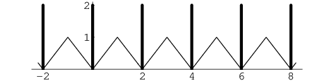
AH is obviously absurd, but it has not been disproven. A sufficiently strong disproof would show that there are no Landau-Siegel zeros. AH implies that Montgomery’s function F⁡(α,T)F(\alpha;T) is periodic with period two. Thus, on AH the graph of F⁡(α,T)F(\alpha;T) would look like this:

Refer to caption
Figure 2. F⁡(α,T)F(\alpha;T) on the Alternative Hypothesis (the heavy vertical lines represent the Dirac δ\delta-functions at the even integers).

Similarly, the triple correlation function form factor F⁡(α,β,T)F(\alpha,\beta;T) (see [12, 18, 9]) would be periodic with period two in both α\alpha and β\beta. Unfortunately, this does not seem to completely determine F⁡(α,β,T)F(\alpha,\beta;T) because F⁡(α,β,T)F(\alpha,\beta;T) is only known on the hexagon |α|<1|\alpha|<1, |β|<1|\beta|<1, |α−β|<1|\alpha-\beta|<1.

If we let gμg_{\mu} denote the proportion of γ~0\tilde{\gamma}_{0} such that γ~0+−γ~0=μ\tilde{\gamma}_{0}^{+}-\tilde{\gamma}_{0}=\mu, a straightforward calculation assuming AH leads to g0=0g_{0}=0, g12=12−2π2≈0.297g_{\frac{1}{2}}=\frac{1}{2}-\frac{2}{\pi^{2}}\approx 0.297, and 0.405≈4π2≤g1≤120.405\approx\frac{4}{\pi^{2}}\leq g_{1}\leq\frac{1}{2}. Thus, one could disprove AH by showing that more than 30% of the normalized neighbor gaps of ξ\xi are less than 0.9990.999. We note that RMT predicts that 53.39% of the neighbor gaps are smaller than average. Montgomery’s result implies that more than 12.3% of the neighbor gaps are smaller than average (set λ=1−ε\lambda=1-\varepsilon at the bottom of page 192 of [16]). Corollary 1.2 gives information about consecutive small gaps between zeros of ξ\xi. This is discussed further in the next subsection.

One wonders whether AH and the existing results on zero correlations determine the distribution of neighbor spacings. To specify g1g_{1} seems to require using the triple correlation F⁡(α,β,T)F(\alpha,\beta;T) to determine how often two consecutive normalized neighbor gaps of size 12\frac{1}{2} can occur. So this question may be equivalent to the question of whether AH determines all the correlation functions.

Goldston and Montgomery [11] showed that the pair correlation conjecture is equivalent to

(2.3) ∫1X(ψ⁡(x+h)−ψ⁡(x)−h)2​𝑑x∼h​X​log⁡(Xh),\int_{1}^{X}\left(\psi(x+h)-\psi(x)-h\right)^{2}\,dx\sim hX\log\left(\frac{X}{h}\right),

for hh in a certain range depending on XX. Here ψ⁡(x)=∑n≤xΛ⁡(n)\psi(x)=\sum_{n\leq x}\Lambda(n), where Λ\Lambda is the von Mangoldt function: Λ⁡(n)=log⁡p\Lambda(n)=\log p if n=pmn=p^{m} with pp prime, and 00 otherwise. Montgomery and Soundararajan [17] interpret (2.3) as saying ψ⁡(x+h)−ψ⁡(x)\psi(x+h)-\psi(x) has mean hh and variance h​log⁡(Xh)h\log\left(\frac{X}{h}\right), and they note that the Cramér model of the primes predicts a larger variance of h​log⁡Xh\log{X}. It would be interesting to see what the right-hand side of (2.3) equals if one assumes the Alternative Hypothesis.

These connections indicate the value of studying the statistics of the zeros of the zeta-function. We now explain the connection to the zeros of ξ′\xi^{\prime}.

2.2. Zeros of derivatives

The statistics of the zeros of ξ′\xi^{\prime} are interesting because of their connection with the Alternative Hypothesis and also as an illustration of the general behavior of the zeros of derivatives of an entire function upon repeated differentiation.

One motivation for studying the analogue of Montgomery’s function for the zeros of ξ′\xi^{\prime} is the expectation that our Theorem 1.1 might contradict AH. The zeros of ξ′\xi^{\prime} are influenced by the zeros of ξ\xi in complicated ways, so it seems unlikely that RMT and AH would predict the same behavior for F1​(α,T)F_{1}(\alpha;T) for |α|<1|\alpha|<1. But there are several caveats. First, as described in the previous section, it is not known whether or not AH determines all the correlation functions of the zeros. This may lead to some flexibility in F1​(α,T)F_{1}(\alpha;T) for |α|<1|\alpha|<1, which may be consistent with Theorem 1.1. Second, it is not known how to transfer a measure on the zeros of ξ\xi to a measure on the zeros of ξ′\xi^{\prime}. Thus, even if AH determined all the correlations of the zeros of ξ\xi, it is still an unsolved problem to determine the correlations of the zeros of ξ′\xi^{\prime}. Third, merely contradicting AH is not sufficient to disprove the existence of Landau-Siegel zeros. AH is an extreme example of a possible consequence of Landau-Siegel zeros. Presumably an extension of the work of Conrey and Iwaniec [4] would show that Landau-Siegel zeros imply that F⁡(α,T)F(\alpha;T) approximately follows Figure 2 for some range of α\alpha.

Another motivation is to understand the general behavior of zeros under differentiation. The Riemann Ξ\Xi-function is defined as Ξ⁡(z)=ξ⁡(12+i​z)\Xi(z)=\xi(\frac{1}{2}+iz). The Ξ\Xi-function is an entire function of order 1 that is real on the real axis. For such functions, repeated differentiation causes the zeros to migrate to the real axis [6, 15, 14]. Thus, in any bounded region the Riemann Hypothesis is true for the nnth derivative Ξ(n)​(z)\Xi^{(n)}(z) for sufficiently large nn.

It is conjectured [8] that for real entire functions of order 1, whose zeros lie in a strip around the real axis, not only do the zeros migrate toward the real axis, but they also approach equal spacing. That is, the derivatives approach a multiple of ea​x​cos⁡(b​x+c)e^{ax}\cos(bx+c). This conjecture has been proven with some restrictions on the distribution of zeros [8] and for some special cases, such as the Ξ\Xi-function [13] and the reciprocal of the gamma function [1].

The reason differentiation leads to equally spaced zeros is that, locally, the zeros of f′f^{\prime} move away from concentrations of zeros of ff and towards regions with fewer zeros of ff. Thus, small gaps become larger and large gaps become smaller. Figure 3 illustrates these ideas.

Refer to caption
Figure 3. The circles are the midpoints of neighboring zeros of ff, and the dots are the zeros of f′f^{\prime}.

A consequence is that if ξ′\xi^{\prime} has a small gap between consecutive zeros, then ξ\xi must have had an even smaller gap. Thus, one should expect that the existence of Landau-Siegel zeros could be disproven by showing that ξ′\xi^{\prime} has sufficiently many zeros separated by less than half the average spacing. That is, one should be able to extend the result of Conrey-Iwaniec [4] to the zeros of ξ(n)\xi^{(n)} for any n≥1n\geq 1. However, we have not worked out the necessary details to show that the required number of small gaps between zeros of ξ′\xi^{\prime} leads to the same number of small gaps between the zeros of ξ\xi. Thus, at present we just mention this as a motivating principle. See [8] for a discussion.

Based on these ideas, we see that Corollary 1.2 does not contradict the Alternative Hypothesis. On average each normalized gap of size 12\frac{1}{2} is adjacent to a gap of size 12\frac{1}{2} or 11, so AH implies that at least 29.7% of the normalized neighbor gaps of ξ′\xi^{\prime} are smaller than 1. If Corollary 1.2 could be improved to show that ξ′\xi^{\prime} has normalized zero gaps smaller than 0.750.75, then that would imply, on AH, that ξ\xi has consecutive gaps of size 12\frac{1}{2}.

Our final motivation is to understand the manner in which differentiation causes the zeros to become equally spaced. Let FnF_{n} denote the analogue of F1F_{1} involving the zeros of ξ(n)​(z)\xi^{(n)}(z) rather than the zeros of  ξ′​(z)\xi^{\prime}(z). Since the zeros of ξ(n)​(z)\xi^{(n)}(z) approach equal spacing as nn increases, FnF_{n} approaches a sum of Dirac δ\delta-functions supported at the integers. We would like to understand this transition to a sum of δ\delta-functions. The only case we know of where this has been worked out explicitly is for random trigonometric polynomials [10]. Theorem 1.1 is a first step in this direction, and Figure 1 does seem to illustrate the expected behavior. In a recent Ph.D. thesis, Jim Bian has now worked out explicit formulas for Fn​(α,T)F_{n}(\alpha;T) for n≥2n\geq 2 and |α|<1|\alpha|<1.

2.3. Connection to RMT

It would be interesting to know the random matrix analogue of Theorem 1.1. At present, this is one of the few calculations carried out for the Riemann zeta-function for which a random matrix analogue seems out of reach. One issue is that in the random matrix world there seems to be no direct analogue of the Riemann ξ\xi-function. See Section 1.2 of [3] for a discussion. The closest match is

(2.4) z−n/2Λ(z),z^{-n/2}\Lambda(z),

where Λ⁡(z)\Lambda(z) is the characteristic polynomial of a random matrix from the unitary group U⁡(n)U(n), chosen uniformly with respect to Haar measure. However, this is more nearly an analogue of the Hardy ZZ-function defined by Z⁡(t)=χ​(12+i​t)−12​ζ​(12+i​t)Z(t)=\chi(\frac{1}{2}+it)^{-\frac{1}{2}}\zeta(\frac{1}{2}+it). This was the motivation of Conrey and Soundararajan [5], who did similar calculations to ours for the ZZ-function. But it turns out that the zeros of Ξ′​(t)\Xi^{\prime}(t) and Z′​(t)Z^{\prime}(t) should have similar correlation functions. Since Ξ⁡(t)\Xi(t) is approximately e−π​t2​Z​(t)e^{-\frac{\pi t}{2}}Z(t), the corresponding zeros of Ξ′​(t)\Xi^{\prime}(t) and Z′​(t)Z^{\prime}(t) generally differ by O⁡(1/log2⁡t)O(1/\log^{2}t). So one should expect the correlation functions of their zeros to be equal, to leading order. We provide a more rigorous explanation in Section 7.2. And those correlation functions should equal, to leading order, the correlation function of the zeros of the derivative of the completed characteristic polynomial (2.4).

3. An explicit formula and first steps of the proof

The general outline of our calculation is similar to the case of zeros of the zeta-function. We start with an explicit formula relating a sum over zeros of ξ′\xi^{\prime} to a sum involving number-theoretic expressions, and then compute the mean-square of both sides. Our main complication is that the number-theoretic side of the explicit formula is not a Dirichlet series, but an “approximate” Dirichlet series, by which we mean a Dirichlet series whose coefficients may depend on ss.

The explicit formula is derived in Section 7. Here we just outline the calculation and state the formula.

We begin by noting that ξ′′/ξ′​(s)\xi^{\prime\prime}/\xi^{\prime}(s) has simple poles with residue 1 at the zeros of ξ′​(s)\xi^{\prime}(s) and no others; here zeros are counted as many times as their multiplicity. Our first goal is to write ξ′′/ξ′​(s)\xi^{\prime\prime}/\xi^{\prime}(s) as an “approximate” Dirichlet series. From the definition of the ξ\xi-function (1.1) we have

(3.1) ξ′ξ​(s)=L​(s)+ζ′ζ​(s),\frac{\xi^{\prime}}{\xi}(s)=L(s)+\frac{\zeta^{\prime}}{\zeta}(s)\;,

where

(3.2) L⁡(s)=\displaystyle L(s)=\mathstrut 1s+1s−1−log⁡π2+12​Γ′Γ​(s2)\displaystyle\frac{1}{s}+\frac{1}{s-1}-\frac{\log\pi}{2}+\frac{1}{2}\frac{\Gamma^{\prime}}{\Gamma}\left(\frac{s}{2}\right)
(3.3) =\displaystyle=\mathstrut 12​log⁡s2​π+O⁡(1|s|+2)\displaystyle\frac{1}{2}\log\frac{s}{2\pi}+O\left(\frac{1}{|s|+2}\right)

and

(3.4) L′​(s)≪1|s|+2L^{\prime}(s)\ll\frac{1}{|s|+2}

in the region |arg⁡s|<π−δ|\arg s|<\pi-\delta, |s|≥1/4|s|\geq 1/4, say.

Multiplying both sides of (3.1) by ξ⁡(s)\xi(s) and calculating the logarithmic derivative leads to the following lemma, the proof of which is in Section 7.

Lemma 3.1.

For σ≥1+ε\sigma\geq 1+\varepsilon, |t|≥Tε|t|\geq T_{\varepsilon}, and KK a large positive integer we have

(3.5) ξ′′ξ′​(s)=L⁡(s)+∑n=1∞aK​(n,s)ns+O⁡(1ε2​2K).\frac{\xi^{\prime\prime}}{\xi^{\prime}}(s)=L(s)+\sum^{\infty}_{n=1}\frac{a_{K}(n,s)}{n^{s}}+O\left(\frac{1}{\varepsilon^{2}2^{K}}\right)\;.

Here we have written

(3.6) aK​(n,s)=∑k=0Kαk​(n)L​(s)k,a_{K}(n,s)=\sum^{K}_{k=0}\frac{\alpha_{k}(n)}{L(s)^{k}},

where

(3.7) αj​(n)={−Λ⁡(n)ifj=0,Λj−1∗Λ​log⁡(n)ifj≥1.\alpha_{j}(n)=\begin{cases}-\Lambda(n)&\quad\hbox{if}\quad j=0,\cr\Lambda_{j-1}*\Lambda\log(n)&\quad\hbox{if}\quad j\geq 1.\end{cases}

The function Λj\Lambda_{j} for j≥0j\geq 0 is the jj-fold convolution of the von Mangoldt function, defined by

(3.8) (−ζ′ζ​(s))j=∑n=1∞Λj​(n)ns.\left(-\frac{\zeta^{\prime}}{\zeta}(s)\right)^{j}=\sum^{\infty}_{n=1}\frac{\Lambda_{j}(n)}{n^{s}}\,.

for σ>1\sigma>1. Simple estimates of Λj\Lambda_{j} and αk\alpha_{k} will be used repeatedly. We have the trivial bound

(3.9) Λj​(n)≤(log⁡n)j(j=1,2,…),\Lambda_{j}(n)\leq(\log n)^{j}\qquad(j=1,2,\dots)\,,

which follows from iterating

(3.10) Λj​(n)=∑d|nΛ⁡(d)​Λj−1​(nd)≤(maxd|n⁡Λj−1​(nd))​∑d|nΛ⁡(d)≤Λj−1​(n∗)​log⁡n\Lambda_{j}(n)=\sum_{d|n}\Lambda(d)\Lambda_{j-1}\left(\frac{n}{d}\right)\leq\left(\max_{d|n}\Lambda_{j-1}\left(\frac{n}{d}\right)\right)\sum_{d|n}\Lambda(d)\leq\Lambda_{j-1}(n^{*})\log n

for some divisor n∗n^{*} of nn. Similarly,

(3.11) αk​(n)=Λk−1∗Λ​log⁡(n)≤(log⁡n)k+1(k=1,2,…),\alpha_{k}(n)=\Lambda_{k-1}*\Lambda\log(n)\leq(\log n)^{k+1}\qquad(k=1,2,\dots)\,,

from which it follows that

(3.12) |aK​(n,s)|≤log⁡n​∑k=0K(log⁡n|L⁡(s)|)k≪logK+1⁡n|a_{K}(n,s)|\leq\log n\sum^{K}_{k=0}\left(\frac{\log n}{|L(s)|}\right)^{k}\ll\log^{K+1}n

when −1≤σ≤2-1\leq\sigma\leq 2, say.

A contour integral of ξ′′/ξ′\xi^{\prime\prime}/\xi^{\prime} times an appropriate kernel leads to the following explicit formula; the details are in Section 7.

Proposition 3.2.

For 5/4<σ<25/4<\sigma<2, x≥1x\geq 1, 0<ε<1/80<\varepsilon<1/8, and KK a positive integer

(3.13) (2σ−1)∑γ\displaystyle(2\sigma-1)\sum_{\gamma} xi​γ(σ−1/2)2+(t−γ)2\displaystyle\frac{x^{{\mathrm{i}}\gamma}}{(\sigma-1/2)^{2}+(t-\gamma)^{2}}
=\displaystyle= x−1/2(∑n≤xaK(n,1−s¯)(xn)1−s¯+∑n>xaK(n,s)(xn)s)\displaystyle x^{-1/2}\left(\sum_{n\leq x}a_{K}(n,1-\bar{s})\left(\frac{x}{n}\right)^{1-\bar{s}}+\sum_{n>x}a_{K}(n,s)\left(\frac{x}{n}\right)^{s}\right)
+x1/2−s¯​log⁡τ2​π+O⁡(x1/2−σ)+Oε,K​(x1/2​τ−1​max⁡(xε,log2​K+2⁡x)),\displaystyle+x^{1/2-\bar{s}}\log\frac{\tau}{2\pi}+O(x^{1/2-\sigma})+O_{\varepsilon,K}\left(x^{1/2}\tau^{-1}\max(x^{\varepsilon},\log^{2K+2}x)\right)\,,

where τ=|t|+2\tau=|t|+2.

4. Beginning of the Proof

Set σ=3/2\sigma=3/2 in Proposition 3.2, write the resulting equation as L⁡(x,t)=R1​(x,t)+R2​(x,t)+R3​(x,t)+R4​(x,t)L(x,t)=R_{1}(x,t)+R_{2}(x,t)+R_{3}(x,t)+R_{4}(x,t), and calculate

(4.1) ∫0T|L⁡(x,t)|2​𝑑t=∫0T|R1​(x,t)+R2​(x,t)+R3​(x,t)+R4​(x,t)|2​𝑑t.\int_{0}^{T}|L(x,t)|^{2}{\mathrm{d}}t=\int_{0}^{T}|R_{1}(x,t)+R_{2}(x,t)+R_{3}(x,t)+R_{4}(x,t)|^{2}{\mathrm{d}}t\,.

The left-hand side may be treated in exactly the same way as the corresponding expression in Montgomery [16], to whom we refer the reader (cf. pp. 187–188). We find

(4.2) ∫0T|L⁡(x,t)|2​𝑑t=2​π​∑0<γ,γ′≤Txi⁡(γ−γ′)​w​(γ−γ′)+O⁡(log3⁡T),\int_{0}^{T}|L(x,t)|^{2}{\mathrm{d}}t=2\pi\sum_{0<\gamma,\gamma^{\prime}\leq T}x^{{\mathrm{i}}(\gamma-\gamma^{\prime})}w(\gamma-\gamma^{\prime})+O(\log^{3}T)\;,

where w⁡(u)=4/(4+u2)w(u)=4/(4+u^{2}).

Next we begin the calculation of the right-hand side of (4.1). In various ranges of xx, one or another of the integrals ∫0T|Ri​(x,t)|2​𝑑t\int_{0}^{T}|R_{i}(x,t)|^{2}{\mathrm{d}}t dominates the others, and we record the following useful formula for later. Given xx, let ℛ𝟏​(x){\bf\mathcal{R}_{1}}(x) be the largest of ∫0T|Ri​(x,t)|2​𝑑t​(i=1,2,3,4)\int_{0}^{T}|R_{i}(x,t)|^{2}{\mathrm{d}}t\;(i=1,2,3,4), ℛ𝟐​(x){\bf\mathcal{R}_{2}}(x) the next largest, and so on. Then we have

(4.3) ∫0T|R1​(x,t)+R2​(x,t)+R3​(x,t)+R4​(x,t)|2​𝑑t=ℛ𝟏​(x)+O⁡((ℛ𝟏​(x)​ℛ𝟐​(x))1/2)\int_{0}^{T}|R_{1}(x,t)+R_{2}(x,t)+R_{3}(x,t)+R_{4}(x,t)|^{2}{\mathrm{d}}t={\bf\mathcal{R}_{1}}(x)+O\left(\left({\bf\mathcal{R}_{1}}(x){\bf\mathcal{R}_{2}}(x)\right)^{1/2}\right)

We find

(4.4) ∫0T|R2​(x,t)|2​𝑑t=∫0T|x−1+i​t​log⁡τ2​π|2​𝑑t=Tx2​(log2⁡T+O⁡(log⁡T)),\int_{0}^{T}|R_{2}(x,t)|^{2}{\mathrm{d}}t=\int^{T}_{0}\left|x^{-1+{\mathrm{i}}t}\log\frac{\tau}{2\pi}\right|^{2}{\mathrm{d}}t=\frac{T}{x^{2}}\left(\log^{2}T+O(\log T)\right)\,,
(4.5) ∫0T|R3​(x,t)|2​𝑑t≪Tx2\int_{0}^{T}|R_{3}(x,t)|^{2}{\mathrm{d}}t\ll\frac{T}{x^{2}}\,

and

(4.6) ∫0T|R4​(x,t)|2​𝑑t\displaystyle\int_{0}^{T}|R_{4}(x,t)|^{2}{\mathrm{d}}t ≪ε,Kxmax(x2​ε,(logx)4​K+4)∫0Td​tτ2\displaystyle\ll_{\varepsilon,K}x\max(x^{2\varepsilon},(\log x)^{4K+4})\int_{0}^{T}\frac{{\mathrm{d}}t}{\tau^{2}}
≪ε,Kxmax(x2​ε,(logx)4​K+4).\displaystyle\ll_{\varepsilon,K}x\max(x^{2\varepsilon},(\log x)^{4K+4})\;.

To estimate ∫0T|R1​(x,t)|2​𝑑t\int_{0}^{T}|R_{1}(x,t)|^{2}{\mathrm{d}}t, we need the following

Lemma 4.1.

Let σ=−1/2\sigma=-1/2 or 3/23/2. Then for x>0x>0 we have

(4.7) ∫0Txi​tL⁡(s)¯k​L​(s)ℓ​𝑑t={T​(12​log⁡(T2​π))−(k+l)​(1+OK​(1log⁡T))if​x=1,OK​(1|log⁡x|)if​x≠1,\displaystyle\int^{T}_{0}\frac{x^{{\mathrm{i}}t}}{\overline{L(s)}\,^{k}L(s)^{\ell}}\;{\mathrm{d}}t=\begin{cases}T\left(\frac{1}{2}\log\left(\frac{T}{2\pi}\right)\right)^{-(k+l)}\left(1+O_{K}\left(\frac{1}{\log T}\right)\right)&\text{if}\;x=1\,,\\ O_{K}\left(\frac{1}{|\log x|}\right)&\text{if}\;x\neq 1\,,\end{cases}

where k,ℓ=0,1,2,…,Kk,\ell=0,1,2,\dotsc,K. The same result holds for

(4.8) ∫0Txi​tL⁡(1−s¯)¯k​L​(s)ℓ​𝑑t.\int^{T}_{0}\frac{x^{{\mathrm{i}}t}}{\overline{L(1-\bar{s})}\,^{k}L(s)^{\ell}}\;{\mathrm{d}}t\;.
Proof.

We prove (4.7) only, as the proof of (4.8) is almost identical.

First observe that from (3.2) we have

(4.9) 1L⁡(s)¯k​L​(s)ℓ=1(12​log⁡τ/2​π)k+l​(1+OK​(1log⁡τ)).\frac{1}{\overline{L(s)}\,^{k}L(s)^{\ell}}=\frac{1}{\left(\frac{1}{2}\log\tau/2\pi\right)^{k+l}}\left(1+O_{K}\left(\frac{1}{\log\tau}\right)\right)\;.

The case x=1x=1 follows immediately.

Now suppose that x>0x>0, but x≠1x\neq 1. Integrating by parts, we find that our integral equals

xi​ti​log⁡x​L⁡(s)¯k​L​(s)ℓ|0T+1i​log⁡x​∫0Txi​tL⁡(s)¯k​L​(s)ℓ​(k​L′¯​(s)L¯​(s)+ℓ​L′​(s)L⁡(s))​𝑑t.\frac{x^{{\mathrm{i}}t}}{{\mathrm{i}}\log x\,\overline{L(s)}\,^{k}L(s)^{\ell}}\bigg|^{T}_{0}+\frac{1}{{\mathrm{i}}\log x}\int^{T}_{0}\frac{x^{{\mathrm{i}}t}}{\overline{L(s)}\,^{k}L(s)^{\ell}}\left(k\frac{\overline{L^{\prime}}(s)}{\overline{L}(s)}+\ell\frac{L^{\prime}(s)}{L(s)}\right){\mathrm{d}}t\;.

By (3.2), (3.4), and (4.9), this is

≪1|log⁡x|​(1+(k+ℓ)​∫0T1τ​(1/2​log⁡τ/2​π)k+ℓ+1​𝑑t)\displaystyle\ll\frac{1}{|\log x|}\left(1+(k+\ell)\int_{0}^{T}\;\frac{1}{\tau(1/2\log\tau/2\pi)^{k+\ell+1}}{\mathrm{d}}t\right)
≪K1|log⁡x|.\displaystyle\ll_{K}\frac{1}{|\log x|}\,.

This completes the proof.

∎

We now come to the term

∫0T|R1​(x,t)|2​𝑑t\displaystyle\int_{0}^{T}|R_{1}(x,t)|^{2}{\mathrm{d}}t =1x∫0T|∑n≤xaK(n,−1/2+it)(xn)−1/2+it+∑n>xaK(n,3/2+it)(xn)3/2+i​t|2dt\displaystyle=\frac{1}{x}\int^{T}_{0}\left|\sum_{n\leq x}a_{K}(n,-1/2+{\mathrm{i}}t)\left(\frac{x}{n}\right)^{-1/2+{\mathrm{i}}t}+\sum_{n>x}a_{K}(n,3/2+{\mathrm{i}}t)\left(\frac{x}{n}\right)^{3/2+{\mathrm{i}}t}\right|^{2}{\mathrm{d}}t
=1x2∫0T|∑n≤xaK(n,−1/2+it)n1/2−i​t|2dt+x2∫0T|∑n>xaK(n,3/2+it)n−3/2−it|2dt\displaystyle=\frac{1}{x^{2}}\int^{T}_{0}\left|\sum_{n\leq x}a_{K}(n,-1/2+{\mathrm{i}}t)n^{1/2-{\mathrm{i}}t}\right|^{2}{\mathrm{d}}t+x^{2}\int^{T}_{0}\left|\sum_{n>x}a_{K}(n,3/2+{\mathrm{i}}t)n^{-3/2-{\mathrm{i}}t}\right|^{2}{\mathrm{d}}t
+2Re∫0T(∑n≤xaK(n,−1/2+it)n1/2−i​t)¯(∑m>xaK(m,3/2+it)m−3/2+it)dt\displaystyle\quad+2Re\,\int^{T}_{0}\overline{\left(\sum_{n\leq x}a_{K}(n,-1/2+{\mathrm{i}}t)n^{1/2-{\mathrm{i}}t}\right)}\left(\sum_{m>x}a_{K}(m,3/2+{\mathrm{i}}t)m^{-3/2+{\mathrm{i}}t}\right){\mathrm{d}}t
=1x2​R1,1+x2​R1,2+2​Re​R1,3,\displaystyle=\frac{1}{x^{2}}R_{1,1}+x^{2}R_{1,2}+2\,{\rm{Re}}\,R_{1,3}\;,

say. Recalling that aK​(n,s)=∑k=0Kαk​(n)/L​(s)k,a_{K}(n,s)=\sum^{K}_{k=0}\alpha_{k}(n)/L(s)^{k}, we see by Lemma 4.1 that

R1,1\displaystyle R_{1,1} =∑m,n≤xm​n​∑k,ℓ=0Kαk​(n)¯​αℓ​(m)​∫0T(n/m)i​tL(−1/2+it)k¯L(−1/2+it)ℓ​𝑑t\displaystyle=\sum_{m,n\leq x}\sqrt{mn}\sum^{K}_{k,\ell=0}\overline{\alpha_{k}(n)}\alpha_{\ell}(m)\int^{T}_{0}\frac{(n/m)^{it}}{\overline{L(-1/2+it)^{k}}L(-1/2+it)^{\ell}}\;dt
=(1+o⁡(1))​T​∑n≤xn⁡(∑k,ℓ=0Kαk​(n)¯​αℓ​(n)(1/2​log⁡T/2​π)k+ℓ)\displaystyle=(1+o(1))T\sum_{n\leq x}n\left(\sum^{K}_{k,\ell=0}\frac{\overline{\alpha_{k}(n)}\alpha_{\ell}(n)}{(1/2\log T/2\pi)^{k+\ell}}\right)
+OK​(∑1≤m<n≤xm​n​(∑k,ℓ=0K|αk​(n)​αℓ​(m)|log⁡n/m))\displaystyle\qquad+O_{K}\left(\sum_{1\leq m<n\leq x}\sqrt{mn}\left(\sum^{K}_{k,\ell=0}\frac{|\alpha_{k}(n)\alpha_{\ell}(m)|}{\log n/m}\right)\right)
=(1+o⁡(1))​T​∑n≤xn​|∑k=0Kαk​(n)(1/2​log⁡T/2​π)k|2\displaystyle=(1+o(1))T\sum_{n\leq x}n\left|\sum^{K}_{k=0}\frac{\alpha_{k}(n)}{(1/2\log T/2\pi)^{k}}\right|^{2}
+OK​(∑1≤m<n≤xm​nlog⁡n/m​(∑k=0K|αk​(n)|)​(∑k=0K|αk​(m)|)).\displaystyle\qquad+O_{K}\left(\sum_{1\leq m<n\leq x}\frac{\sqrt{mn}}{\log n/m}\left(\sum^{K}_{k=0}|\alpha_{k}(n)|\right)\left(\sum^{K}_{k=0}|\alpha_{k}(m)|\right)\right)\;.

From the standard inequality

(4.10) ∑1≤m<n≤x|b⁡(m)​b​(n)|(m​n)σ​log⁡n/m≪x​log⁡x​∑n≤x|b⁡(n)|2n2​σ\sum_{1\leq m<n\leq x}\frac{|b(m)b(n)|}{(mn)^{\sigma}\log n/m}\ll x\log x\sum_{n\leq x}\,\frac{|b(n)|^{2}}{n^{2\sigma}}

and (3.11) we see that the OO-term is

≪Kxlogx∑n≤xn(∑k=0K|αk(n)|)2\displaystyle\ll_{K}x\log x\sum_{n\leq x}n\left(\sum^{K}_{k=0}|\alpha_{k}(n)|\right)^{2}
≪Kxlogx∑n≤xn(logn)2​K+2\displaystyle\ll_{K}x\log x\sum_{n\leq x}n(\log n)^{2K+2}
≪Kx3(logx)2​K+3.\displaystyle\ll_{K}x^{3}(\log x)^{2K+3}\;.

Thus, we have

R1,1=(1+o⁡(1))​T​∑n≤xn​|∑k=0Kαk​(n)(1/2​log⁡T/2​π)k|2+OK​(x3​(log⁡x)2​K+3).R_{1,1}=(1+o(1))T\sum_{n\leq x}n\left|\sum^{K}_{k=0}\frac{\alpha_{k}(n)}{(1/2\log T/2\pi)^{k}}\right|^{2}+O_{K}\left(x^{3}(\log x)^{2K+3}\right)\;.

Similarly, we find that

R1,2=(1+o⁡(1))​T​∑n>xn−3​|∑k=0Kαk​(n)(1/2​log⁡T/2​π)k|2+OK​(x−1​(log⁡x)2​K+3).R_{1,2}=(1+o(1))T\sum_{n>x}n^{-3}\left|\sum^{K}_{k=0}\frac{\alpha_{k}(n)}{(1/2\log T/2\pi)^{k}}\right|^{2}+O_{K}\left(x^{-1}(\log x)^{2K+3}\right)\;.

For R1,3R_{1,3} we have

R1,3\displaystyle R_{1,3} =∑n≤xn1/2∑m>xm−3/2∑k,ℓ=0Kαk​(n)¯αℓ(m)∫0T(m​n)i​tL(−1/2+it)¯k​L​(3/2+i​t)ℓdt\displaystyle=\sum_{n\leq x}n^{1/2}\sum_{m>x}m^{-3/2}\sum^{K}_{k,\ell=0}\overline{\alpha_{k}(n)}\alpha_{\ell}(m)\int^{T}_{0}\frac{(mn)^{it}}{\overline{L(-1/2+it)}\,^{k}L(3/2+it)^{\ell}}\,dt
≪∑n≤xn1/2∑m>xm−3/2(logmn)−1(∑k,ℓ=0K|αk(n)αℓ(m)|)\displaystyle\ll\sum_{n\leq x}n^{1/2}\sum_{m>x}m^{-3/2}(\log mn)^{-1}\left(\sum^{K}_{k,\ell=0}|\alpha_{k}(n)\alpha_{\ell}(m)|\right)
≪K∑n≤x∑m>xn1/2m−3/2log⁡m​n(logm)K+1(logn)K+1\displaystyle\ll_{K}\sum_{n\leq x}\sum_{m>x}\frac{n^{1/2}m^{-3/2}}{\log mn}(\log m)^{K+1}(\log n)^{K+1}
≪K1log⁡x(∑n≤xn1/2(logn)K+1)(∑m>xm−3/2(logm)K+1)\displaystyle\ll_{K}\frac{1}{\log x}\left(\sum_{n\leq x}n^{1/2}(\log n)^{K+1}\right)\left(\sum_{m>x}m^{-3/2}(\log m)^{K+1}\right)
≪Kx(logx)2​K+1.\displaystyle\ll_{K}x(\log x)^{2K+1}\;.

Combining these estimates, we have

(4.11) ∫0T|R1​(x,t)|2​dt=\displaystyle\int_{0}^{T}|R_{1}(x,t)|^{2}{\mathrm{d}}t= (1+o⁡(1))​T​x−2​∑n≤xn​|∑k=0Kαk​(n)(1/2​log⁡T/2​π)k|2\displaystyle(1+o(1))Tx^{-2}\sum_{n\leq x}n\left|\sum^{K}_{k=0}\;\frac{\alpha_{k}(n)}{(1/2\log T/2\pi)^{k}}\right|^{2}
+(1+o(1))Tx2∑n>x1n3|∑Kk=0αk​(n)(1/2​log⁡T/2​π)k|2\displaystyle+(1+o(1))Tx^{2}\sum_{n>x}\frac{1}{n^{3}}\left|\sum^{K}_{k=0}\frac{\alpha_{k}(n)}{(1/2\log T/2\pi)^{k}}\right|^{2}
+OK​(x​(log⁡x)2​K+3).\displaystyle+O_{K}(x(\log x)^{2K+3})\;.

In the next section we complete the proof of Theorem 1.1, subject to an arithmetic proposition which we prove in Section 6.

5. Proof of Theorem 1.1

It remains to evaluate (4.11) and to put the expressions in the form of Theorem 1.1. The main terms from (4.11) can be obtained from a Stieltjes integral involving

(5.1) A⁡(x)=A⁡(x,K,T)=∑n≤x|∑k=0Kαk​(n)ℒk|2.A(x)=A(x,K,T)=\sum_{n\leq x}\left|\sum^{K}_{k=0}\frac{\alpha_{k}(n)}{\mathcal{L}^{k}}\right|^{2}.

Here αk\alpha_{k} is defined in (3.7) and ℒ=12​log⁡T2​π\mathcal{L}=\frac{1}{2}\log\frac{T}{2\pi}. We write

(5.2) A⁡(x)=∑k=0KAk,k​(x)​ℒ−2​k+2​∑k=1K∑0≤ℓ<kAk,ℓ​(x)​ℒ−(k+ℓ),A(x)=\sum^{K}_{k=0}A_{k,k}(x)\mathcal{L}^{-2k}+2\sum^{K}_{k=1}\sum_{0\leq\ell<k}A_{k,\ell}(x)\mathcal{L}^{-(k+\ell)},

where

(5.3) Ak,ℓ​(x)=∑n≤xαk​(n)​αℓ​(n).A_{k,\ell}(x)=\sum_{n\leq x}\alpha_{k}(n)\alpha_{\ell}(n).

The following proposition, which is proven in Section 6, is sufficient to evaluate the leading order asymptotics of (4.11).

Proposition 5.1.

We have

(5.4) Ak,0​(x)={x​log⁡x+O⁡(x) if k=0,−x​log2​x+O⁡(x​log⁡x) if k=1,O⁡(x12+ε) if k≥2.A_{k,0}(x)=\begin{cases}x\log x+O(x)\quad&\text{ if }\ \ k=0\,,\\ -x\log^{2}x+O(x\log x)\quad&\text{ if }\ \ k=1\,,\\ O\bigl(x^{\tfrac{1}{2}+\varepsilon}\bigr)\quad&\text{ if }\ \ k\geq 2\;.\end{cases}

and

(5.5) Ak,1​(x)={x​log3​x+O⁡(x​log2​x) if k=1,O⁡(x12+ε) if k≥2.A_{k,1}(x)=\begin{cases}x\log^{3}x+O(x\log^{2}x)\quad&\text{ if }\ \ k=1\;,\\ O\bigl(x^{\tfrac{1}{2}+\varepsilon}\bigr)&\text{ if }\ \ k\geq 2\;.\end{cases}

If k≥1k\geq 1, then

(5.6) Ak,k​(x)=2​(k−1)!(2​k)!​x​log2​k+1​x+O⁡(x​log2​k​x),A_{k,k}(x)=2\frac{(k-1)!}{(2k)!}x\log^{2k+1}x+O(x\log^{2k}x),

and if k>ℓ≥2k>\ell\geq 2, then

(5.7) Ak,ℓ​(x)≪x​logk+ℓ​x.A_{k,\ell}(x)\ll x\log^{k+\ell}x.

As a consequence, we have

(5.8) A⁡(x)=x​log⁡x⁡(1−2​(log⁡xℒ)+2​∑k=1K(k−1)!(2​k)!​(log⁡xℒ)2​k)+OK​(x){A}(x)=x\log x\left(1-2\left(\frac{\log x}{\mathcal{L}}\right)+2\sum^{K}_{k=1}\frac{(k-1)!}{(2k)!}\left(\frac{\log x}{\mathcal{L}}\right)^{2k}\right)+O_{K}(x)

for x=Tαx=T^{\alpha} with 0<α≤C00<\alpha\leq C_{0}, where C0C_{0} is any fixed positive number.

Proof of Theorem 1.1.

We first evaluate ∫0T|R1​(x,t)|2​𝑑t\int_{0}^{T}|R_{1}(x,t)|^{2}{\mathrm{d}}t given by (4.11). We have

(5.9) ∫0T|R1​(x,t)|2​𝑑t\displaystyle\int_{0}^{T}|R_{1}(x,t)|^{2}{\mathrm{d}}t =(1+o⁡(1))​T​{x−2​∫1−xu​𝑑A​(u)+x2​∫x∞u−3​𝑑A​(u)}+OK​(x​(log⁡x)2​K+3)\displaystyle=(1+o(1))T\left\{x^{-2}\int^{x}_{1^{-}}u\,d{A}(u)+x^{2}\int^{\infty}_{x}u^{-3}d{A}(u)\right\}+O_{K}\left(x(\log x)^{2K+3}\right)
(5.10) =(1+o(1)T{−x−2∫1xA(u)du+3x2∫x∞u−4A(u)du}+OK(x(logx)2​K+3).\displaystyle=(1+o(1)T\left\{-x^{-2}\int^{x}_{1}{A}(u)du+3x^{2}\int^{\infty}_{x}u^{-4}{A}(u)du\right\}+O_{K}\left(x(\log x)^{2K+3}\right)\;.

Note that the boundary terms canceled when we integrated by parts.

The typical term in the series for A⁡(u){A}(u) has the form C​u​(log⁡u)m+1/ℒmCu(\log u)^{m+1}/\mathcal{L}^{m} and, assuming that m≪Km\ll K, we have

1ℒm​∫1xu​(log⁡u)m+1​𝑑u=1ℒm​x22​(log⁡x)m+1​(1+OK​(1log⁡x))\frac{1}{\mathcal{L}^{m}}\int^{x}_{1}u(\log u)^{m+1}du=\frac{1}{\mathcal{L}^{m}}\frac{x^{2}}{2}(\log x)^{m+1}\left(1+O_{K}\left(\frac{1}{\log x}\right)\right)

and

1ℒm​∫x∞u−3​(log⁡u)m+1​𝑑u=1ℒm​12​x2​(log⁡x)m+1​(1+OK​(1log⁡x)).\frac{1}{\mathcal{L}^{m}}\int^{\infty}_{x}u^{-3}(\log u)^{m+1}du=\frac{1}{\mathcal{L}^{m}}\frac{1}{2x^{2}}(\log x)^{m+1}\left(1+O_{K}\left(\frac{1}{\log x}\right)\right)\;.

Using the first formula and (5.8), we have

−x−2∫1xA(u)du=\displaystyle-x^{-2}\int^{x}_{1}{A}(u)du= −x−2∫1xu(logu−2log2⁡uℒ+2∑k=1K(k−1)!(2​k)!(log⁡u)2​k+1ℒ2​k)du+OK(1)\displaystyle-x^{-2}\int^{x}_{1}u\left(\log u-2\frac{\log^{2}u}{\mathcal{L}}+2\sum^{K}_{k=1}\frac{(k-1)!}{(2k)!}\frac{(\log u)^{2k+1}}{\mathcal{L}^{2k}}\right)du+O_{K}(1)
=\displaystyle= log⁡x⁡{−12+log⁡xℒ−∑k=1K(k−1)!(2​k)!​(log⁡xℒ)2​k}​(1+OK​(1log⁡x))+OK​(1).\displaystyle\log x\left\{-\frac{1}{2}+\frac{\log x}{\mathcal{L}}-\sum^{K}_{k=1}\frac{(k-1)!}{(2k)!}\left(\frac{\log x}{\mathcal{L}}\right)^{2k}\right\}\left(1+O_{K}\left(\frac{1}{\log x}\right)\right)+O_{K}(1)\,.

For x≪TCx\ll T^{C}, the OK​(1/log⁡x)O_{K}(1/\log x) term contributes no more than OK​(1)O_{K}(1) to this. Hence,

(5.11) −x−2∫1xA(u)du=logx(−12+log⁡xℒ−∑k=1K(k−1)!(2​k)!(log⁡xℒ)2​k)+OK(1).-x^{-2}\int^{x}_{1}{A}(u)du=\log x\left(-\frac{1}{2}+\frac{\log x}{\mathcal{L}}-\sum^{K}_{k=1}\frac{(k-1)!}{(2k)!}\left(\frac{\log x}{\mathcal{L}}\right)^{2k}\right)+O_{K}(1)\;.

Similarly, using the second formula and (5.8), we obtain

3​x2​∫x∞u−4​A​(u)​𝑑u\displaystyle 3x^{2}\int^{\infty}_{x}u^{-4}{A}(u)du =3​x2​∫x∞u−3​(log⁡u−2​log2​uℒ+2​∑k=1K(k−1)!(2​k)!​(log⁡u)2​k+1ℒ2​k)​𝑑u+OK​(1)\displaystyle=3x^{2}\int^{\infty}_{x}u^{-3}\left(\log u-\frac{2\log^{2}u}{\mathcal{L}}+2\sum^{K}_{k=1}\frac{(k-1)!}{(2k)!}\frac{(\log u)^{2k+1}}{\mathcal{L}^{2k}}\right)du+O_{K}(1)
(5.12) =log⁡x⁡{32−3​log⁡xL+3​∑k=1K(k−1)!(2​k)!​(log⁡xL)2​k}+OK​(1).\displaystyle=\log x\left\{\frac{3}{2}-3\frac{\log x}{L}+3\sum^{K}_{k=1}\frac{(k-1)!}{(2k)!}\left(\frac{\log x}{L}\right)^{2k}\right\}+O_{K}(1)\,.

Combining terms we obtain

(5.13) ∫0T|R1​(x,t)|2​dt=\displaystyle\int_{0}^{T}|R_{1}(x,t)|^{2}{\mathrm{d}}t= (1+o⁡(1))​T​log⁡x⁡(1−2​log⁡xℒ+2​∑k=1K(k−1)!(2​k)!​(log⁡xℒ)2​k)\displaystyle\left(1+o(1)\right)T\log x\left(1-2\frac{\log x}{\mathcal{L}}+2\sum^{K}_{k=1}\frac{(k-1)!}{(2k)!}\left(\frac{\log x}{\mathcal{L}}\right)^{2k}\right)
+OK​(T)+OK​(x​(log⁡x)2​K+3)\displaystyle+O_{K}(T)+O_{K}\left(x(\log x)^{2K+3}\right)

provided x≪TC0x\ll T^{C_{0}}.

Recall from (4.1) and (4.2) that we write

(5.14) 2​π​∑0<γ,γ′≤Txi⁡(γ−γ′)​w​(γ−γ′)=ℛ1​(x)+O⁡((ℛ1​(x)​ℛ2​(x))1/2)+O⁡(log3⁡T),2\pi\sum_{0<\gamma,\gamma^{\prime}\leq T}x^{{\mathrm{i}}(\gamma-\gamma^{\prime})}w(\gamma-\gamma^{\prime})=\mathcal{R}_{1}(x)+O\left(\left(\mathcal{R}_{1}(x)\mathcal{R}_{2}(x)\right)^{1/2}\right)+O(\log^{3}T)\,,

where, for a given xx, ℛ1​(x)\mathcal{R}_{1}(x) is the largest of ∫0T|Ri​(x,t)|2​𝑑t​(i=1,2,3,4)\int_{0}^{T}|R_{i}(x,t)|^{2}{\mathrm{d}}t\;(i=1,2,3,4) and ℛ2​(x)\mathcal{R}_{2}(x) is the next largest. Now, from the various estimates we see that our ℛ1​(x)\mathcal{R}_{1}(x) term is given by

(1+o⁡(1))​Tx2​log2​T\displaystyle(1+o(1))\frac{T}{x^{2}}\log^{2}T  if ​1≤x≤(log⁡T)3/4,\displaystyle\qquad\hbox{ if }1\leq x\leq(\log T)^{3/4}\;,
o⁡(T​log⁡T)\displaystyle o(T\log T)  if (log⁡T)3/4<x≤(log⁡T)3/2,\displaystyle\qquad\hbox{ if }\quad(\log T)^{3/4}<x\leq(\log T)^{3/2}\;,

and by

(1+oK​(1))​T​log⁡x⁡(1−2​log⁡xℒ+2​∑k=1K(k−1)!(2​k)!​(log⁡xℒ)2​k)\displaystyle\left(1+o_{K}(1)\right)T\log x\left(1-2\frac{\log x}{\mathcal{L}}+2\sum^{K}_{k=1}\frac{(k-1)!}{(2k)!}\left(\frac{\log x}{\mathcal{L}}\right)^{2k}\right)  if (log⁡T)3/2<x≤T1−ε.\displaystyle\qquad\hbox{ if }\quad(\log T)^{3/2}<x\leq T^{1-\varepsilon}\;.

In each of these ranges, it happens that the ℛ2​(x)\mathcal{R}_{2}(x) term is o​(ℛ1​(x))o(\mathcal{R}_{1}(x)). Hence, taking x=Tαx=T^{\alpha} in (5.14), we find that for 0<α<10<\alpha<1 and TT large,

2​π​∑0<γ,γ′≤TTi​α​(γ−γ′)​w​(γ−γ′)\displaystyle 2\pi\,\sum_{0<\gamma,\gamma^{\prime}\leq T}T^{{\mathrm{i}}\alpha(\gamma-\gamma^{\prime})}w(\gamma-\gamma^{\prime})
=(1+o⁡(1))​T1−2​α​log2​T+(1+oK​(1))​α​T​log⁡T⁡(1−4​α+2​∑k=1K(k−1)!(2​k)!​(2​α)2​k)+oK​(1).\displaystyle=(1+o(1))T^{1-2\alpha}\log^{2}T+(1+o_{K}(1))\alpha T\log T\left(1-4\alpha+2\sum^{K}_{k=1}\frac{(k-1)!}{(2k)!}\left(2\alpha\right)^{2k}\right)+o_{K}(1)\;.

Using (1.3) and noting that F1​(α,T)F_{1}(\alpha,T) is an even function of α\alpha, we have proved Theorem 1.1.

∎

6. Proof of Proposition 5.1

We prove Proposition 5.1, which is the arithmetic portion of the calculation. We first reduce Ak,ℓA_{k,\ell} to a sum involving the arithmetic functions Λj\Lambda_{j}. In Section 6.2 we state some lemmas which are needed in the calculation, and in Section 6.3 we evaluate the sums of the Λj\Lambda_{j}. Then we complete the proof of Proposition 5.1 in Section 6.4

6.1. Reduction of Ak,ℓA_{k,\ell}

Recall that

(6.1) Ak,ℓ​(x)=∑n≤xαk​(n)​αℓ​(n),A_{k,\ell}(x)=\sum_{n\leq x}\alpha_{k}(n)\alpha_{\ell}(n),

where αk\alpha_{k} is given by (3.7).

Lemma 6.1.

We have

(6.2) Ak,0​(x)={x​log⁡x+O⁡(x) if k=0,−x​log2​x+O⁡(x​log⁡x) if k=1,O⁡(x12+ε) if k≥2.A_{k,0}(x)=\begin{cases}x\log x+O(x)\quad&\text{ if }\ \ k=0\,,\\ -x\log^{2}x+O(x\log x)\quad&\text{ if }\ \ k=1\,,\\ O\bigl(x^{\tfrac{1}{2}+\varepsilon}\bigr)\quad&\text{ if }\ \ k\geq 2\;.\end{cases}

and

(6.3) Ak,1​(x)={x​log3​x+O⁡(x​log2​x) if k=1,O⁡(x12+ε) if k≥2.A_{k,1}(x)=\begin{cases}x\log^{3}x+O(x\log^{2}x)\quad&\text{ if }\ \ k=1\;,\\ O\bigl(x^{\tfrac{1}{2}+\varepsilon}\bigr)&\text{ if }\ \ k\geq 2\;.\end{cases}

For 2≤ℓ≤k2\leq\ell\leq k we have

(6.4) Ak,ℓ​(x)\displaystyle A_{k,\ell}(x) =(k−1)​(ℓ−1)​∑p≤x∑q≤xplog3⁡p​log3⁡q⁡(∑m≤xp​qΛk−2​(m)​Λℓ−2​(m))\displaystyle=(k-1)(\ell-1)\sum_{p\leq x}\sum_{q\leq\frac{x}{p}}\log^{3}p\,\log^{3}q\left(\sum_{m\leq\frac{x}{pq}}\Lambda_{k-2}(m)\Lambda_{\ell-2}(m)\right)
(6.5) +∑p≤xlog4p(∑m≤xpΛk−1(m)Λℓ−1(m))\displaystyle\quad+\sum_{p\leq x}\log^{4}p\left(\sum_{m\leq\frac{x}{p}}\Lambda_{k-1}(m)\Lambda_{\ell-1}(m)\right)
(6.6) +O⁡(x​logk+ℓ​x).\displaystyle\quad\quad+O(x\log^{k+\ell}x).
Proof.

The form of αk​(n)\alpha_{k}(n) is different when k=0k=0 and 11 from what it is for larger kk, and this will be reflected in our estimates for Ak,ℓ​(x)A_{k,\ell}(x). We therefore treat these cases separately.

First consider the case of Ak,0​(x)A_{k,0}(x). By the prime number theorem we have

(6.7) A0,0​(s)=∑n≤xΛ2​(n)=x​log⁡x+O⁡(x)A_{0,0}(s)=\sum_{n\leq x}\Lambda^{2}(n)=x\log x+O(x)

and

(6.8) A1,0(x)=−∑n≤xΛ2(n)logn=−xlog2x+O(xlogx).A_{1,0}(x)=-\sum_{n\leq x}\Lambda^{2}(n)\log n=-x\log^{2}x+O(x\log x)\,.

For k≥2k\geq 2 we have

(6.9) Ak,0​(x)=\displaystyle A_{k,0}(x)=\mathstrut −∑n≤xΛ(n)(Λk−1∗Λlog)(n)\displaystyle-\sum_{n\leq x}\Lambda(n)(\Lambda_{k-1}*\Lambda\log)(n)
(6.10) =\displaystyle=\mathstrut −∑pa≤xlog(p)(Λk−1∗Λlog)(pa)\displaystyle-\sum_{p^{a}\leq x}\log(p)(\Lambda_{k-1}*\Lambda\log)(p^{a})
(6.11) ≪\displaystyle\ll\mathstrut ∑pa≤xa≥kpa​ε\displaystyle\sum_{\genfrac{}{}{0.0pt}{}{p^a \le x}{a\ge k}}p^{a\varepsilon}
(6.12) ≪\displaystyle\ll\mathstrut x12+ε.\displaystyle x^{\tfrac{1}{2}+\varepsilon}.

We have used the fact that (Λk−1∗Λ​log)​(n)≪nε(\Lambda_{k-1}*\Lambda\log)(n)\ll n^{\varepsilon} and that this function vanishes unless nn is a product of at least kk (not necessarily distinct) primes and k≥2k\geq 2.

Next we consider Ak,1​(x)A_{k,1}(x) for k≥1k\geq 1. By the prime number theorem,

(6.13) A1,1​(x)=∑n≤x(Λ⁡(n)​log⁡n)2=x​log3​x+O⁡(x​log2​x).A_{1,1}(x)=\sum_{n\leq x}(\Lambda(n)\log n)^{2}=x\log^{3}x+O(x\log^{2}x)\;.

If k≥2k\geq 2 then

(6.14) Ak,1​(x)=\displaystyle A_{k,1}(x)=\mathstrut ∑n≤xΛ⁡(n)​log⁡n⁡(Λk−1∗Λ​log)​(n)\displaystyle\sum_{n\leq x}\Lambda(n)\log n\,\left(\Lambda_{k-1}*\Lambda\log\right)(n)
(6.15) ≪\displaystyle\ll\mathstrut x12+ε,\displaystyle x^{\tfrac{1}{2}+\varepsilon},

exactly as in (6.9).

We now come to the general case of Ak,ℓ​(x)A_{k,\ell}(x) with k≥ℓ≥2k\geq\ell\geq 2. We have

(6.16) Ak,ℓ​(x)=\displaystyle A_{k,\ell}(x)=\mathstrut ∑n≤xαk​(n)​αl​(n)\displaystyle\sum_{n\leq x}\alpha_{k}(n)\alpha_{l}(n)
(6.17) =\displaystyle=\mathstrut ∑n≤x(∑pa|na​log2​p​Λk−1​(npa))​(∑qb|nb​log2​q​Λℓ−1​(nqb))\displaystyle\sum_{n\leq x}\left(\sum_{p^{a}|n}a\log^{2}p\;\Lambda_{k-1}\left(\frac{n}{p^{a}}\right)\right)\left(\sum_{q^{b}|n}b\log^{2}q\;\Lambda_{\ell-1}\left(\frac{n}{q^{b}}\right)\right)
(6.18) =\displaystyle=\mathstrut ∑n≤x(∑p|nlog2⁡p​Λk−1​(np))​(∑q|nlog2⁡q​Λℓ−1​(nq))\displaystyle\sum_{n\leq x}\left(\sum_{p|n}\log^{2}p\;\Lambda_{k-1}\left(\frac{n}{p}\right)\right)\left(\sum_{q|n}\log^{2}q\;\Lambda_{\ell-1}\left(\frac{n}{q}\right)\right)
(6.19) +O⁡(x​logk+ℓ​x)\displaystyle\quad+O(x\log^{k+\ell}x)
(6.20) =\displaystyle=\mathstrut ∑p≤x∑q≤xpq≠plog2⁡p​log2⁡q⁡(∑n≤xp​q|nΛk−1​(np)​Λℓ−1​(nq))\displaystyle\sum_{p\leq x}\sum_{\begin{subarray}{c}q\leq\frac{x}{p}\\ q\neq p\end{subarray}}\log^{2}p\log^{2}q\left(\sum_{\begin{subarray}{c}n\leq x\\ pq|n\end{subarray}}\Lambda_{k-1}\left(\frac{n}{p}\right)\Lambda_{\ell-1}\left(\frac{n}{q}\right)\right)
(6.21) +∑p≤xlog4p(∑n≤xp|nΛk−1(np)Λℓ−1(np))\displaystyle\quad+\sum_{p\leq x}\log^{4}p\left(\sum_{\begin{subarray}{c}n\leq x\\ p|n\end{subarray}}\Lambda_{k-1}\left(\frac{n}{p}\right)\Lambda_{\ell-1}\left(\frac{n}{p}\right)\right)
(6.22) +O⁡(x​logk+ℓ​x)\displaystyle\quad+O(x\log^{k+\ell}x)
(6.23) =\displaystyle=\mathstrut A1+A2+O⁡(x​log⁡xk+ℓ​x),\displaystyle{A}_{1}+{A}_{2}+O(x\log x^{k+\ell}x)\;,

say. The estimate on the third line above was done as follows. By symmetry, it is sufficient to estimate

(6.24) ∑pa≤xa≥1∑qb≤xpab≥2a​b​log2​p​log2⁡q⁡(∑m≤xpa​qbΛk−1​(m​qb)​Λℓ−1​(m​pa)).\sum_{\begin{subarray}{c}p^{a}\leq x\\ a\geq 1\end{subarray}}\sum_{\begin{subarray}{c}q^{b}\leq\frac{x}{p^{a}}\\ b\geq 2\end{subarray}}ab\log^{2}p\;\log^{2}q\left(\sum_{m\leq\frac{x}{p^{a}q^{b}}}\Lambda_{k-1}(mq^{b})\;\Lambda_{\ell-1}(mp^{a})\right)\;.

By the trivial bound (3.9) this is

(6.25) ≪\displaystyle\ll\mathstrut ∑pa≤xa≥1∑qb≤xpab≥2a​b​log2​p​log2⁡q⁡(∑m≤xpa​qb(log⁡m​qb)k−1​(log⁡m​pa)ℓ−1)\displaystyle\sum_{\begin{subarray}{c}p^{a}\leq x\\ a\geq 1\end{subarray}}\sum_{\begin{subarray}{c}q^{b}\leq\frac{x}{p^{a}}\\ b\geq 2\end{subarray}}ab\log^{2}p\;\log^{2}q\left(\sum_{m\leq\frac{x}{p^{a}q^{b}}}(\log mq^{b})^{k-1}\;(\log mp^{a})^{\ell-1}\right)
(6.26) ≪\displaystyle\ll\mathstrut x​(log⁡x)k+ℓ−2​∑pa≤xa≥1a​log2​ppa​∑qb≤xpab≥2b​log2​qqb\displaystyle x(\log x)^{k+\ell-2}\sum_{\begin{subarray}{c}p^{a}\leq x\\ a\geq 1\end{subarray}}\frac{a\log^{2}p}{p^{a}}\sum_{\begin{subarray}{c}q^{b}\leq\frac{x}{p^{a}}\\ b\geq 2\end{subarray}}\frac{b\log^{2}q}{q^{b}}
(6.27) ≪\displaystyle\ll\mathstrut x​(log⁡x)k+ℓ−2​∑pa≤xa≥1a​log2​ppa\displaystyle x(\log x)^{k+\ell-2}\sum_{\begin{subarray}{c}p^{a}\leq x\\ a\geq 1\end{subarray}}\frac{a\log^{2}p}{p^{a}}
(6.28) ≪\displaystyle\ll\mathstrut x​(log⁡x)k+ℓ,\displaystyle x(\log x)^{k+\ell},

as claimed. One can use Lemma 6.2 on the inner summand of (6.24) to improve this bound by a power of log⁡x\log x, but this will not affect our final result.

It is clear that A2{A}_{2} equals the second main term in (6.4), so it remains to put A1{A}_{1} in the appropriate form. The point is that if pp is prime and p∤mp\nmid m then

(6.29) Λk​(p​m)=k⁡(log⁡p)​Λk−1​(m).\Lambda_{k}(pm)=k(\log p)\Lambda_{k-1}(m).

See the proof of Lemma 6.2. Thus

(6.30) A1=\displaystyle{A}_{1}=\mathstrut (k−1)​(ℓ−1)​∑p≤x∑q≤xpq≠plog3⁡p​log3⁡q⁡(∑m≤xp​q(m,p​q)=1Λk−2​(m)​Λℓ−2​(m))\displaystyle(k-1)(\ell-1)\sum_{p\leq x}\sum_{\begin{subarray}{c}q\leq\frac{x}{p}\\ q\neq p\end{subarray}}\log^{3}p\,\log^{3}q\left(\sum_{\begin{subarray}{c}m\leq\frac{x}{pq}\\ (m,pq)=1\end{subarray}}\Lambda_{k-2}(m)\Lambda_{\ell-2}(m)\right)
(6.31) +∑p≤x∑q≤xpq≠plog2plog2q(∑m≤xp​q(m,q​p)>1Λk−1(mq)Λℓ−1(mp)).\displaystyle\mathstrut+\sum_{p\leq x}\sum_{\begin{subarray}{c}q\leq\frac{x}{p}\\ q\neq p\end{subarray}}\log^{2}p\,\log^{2}q\left(\sum_{\begin{subarray}{c}m\leq\frac{x}{pq}\\ (m,qp)>1\end{subarray}}\Lambda_{k-1}(mq)\Lambda_{\ell-1}(mp)\right).

The second term can be estimated using the trivial bound (3.9), exactly as in (6.25), showing that it is ≪x​(log⁡x)k+ℓ\ll x(\log x)^{k+\ell}. For the first term, removing the conditions (m,p​q)=1(m,pq)=1 and q≠pq\not=p and estimating with the trivial bound (3.9) gives an even smaller error term. This completes the proof of Lemma 6.1.

∎

6.2. Some lemmas

The following lemmas concerning the Λj\Lambda_{j} function and sums over primes are required in the next subsection.

The first Lemma is an improvement on the trivial bound (3.9) for Λj​(n)\Lambda_{j}(n) when nn has a known prime factor.

Lemma 6.2.

If p|mp|m, then

Λk​(m)≤k​log⁡p​(log⁡m)k−1.\Lambda_{k}(m)\leq k\log p(\log m)^{k-1}.
Proof.

If (p,n)=1(p,n)=1 then

Λk​(pa​n)=∑j=1min⁡(a,k)(kj)​Λj​(pa)​Λk−j​(n)=∑j=1k(kj)​(a−1j−1)​(log⁡p)j​Λk−j​(n).\Lambda_{k}(p^{a}n)=\sum^{\min(a,k)}_{j=1}\binom{k}{j}\Lambda_{j}(p^{a})\Lambda_{k-j}(n)=\sum^{k}_{j=1}\binom{k}{j}\binom{a-1}{j-1}(\log p)^{j}\Lambda_{k-j}(n)\,.

Setting a=1a=1, we obtain (6.29).

Now

(a−1j−1)=(a−1)(a−2)⋯(a−j+1)(j−1)!≤aj−1(j−1)!.\binom{a-1}{j-1}=\frac{(a-1)(a-2)\cdots(a-j+1)}{(j-1)!}\leq\frac{a^{j-1}}{(j-1)!}\;.

Hence

Λk​(pa​n)\displaystyle\Lambda_{k}(p^{a}n) ≤∑j=1kkj​(k−1j−1)​aj−1(j−1)!​(log⁡p)j​(log⁡n)k−j\displaystyle\leq\sum^{k}_{j=1}\frac{k}{j}\binom{k-1}{j-1}\frac{a^{j-1}}{(j-1)!}(\log p)^{j}(\log n)^{k-j}
≤k​log⁡p​∑j=1k(k−1j−1)​(log⁡pa)j−1​(log⁡n)(k−1)−(j−1).\displaystyle\leq k\log p\sum^{k}_{j=1}\binom{k-1}{j-1}(\log p^{a})^{j-1}(\log n)^{(k-1)-(j-1)}\;.

Setting j−1=ij-1=i, this is

=k​log⁡p​∑i=0k−1(k−1i)​(log⁡pa)i​(log⁡n)(k−1)−i\displaystyle=k\log p\sum^{k-1}_{i=0}\binom{k-1}{i}(\log p^{a})^{i}(\log n)^{(k-1)-i}
≤k​log⁡p​(log⁡pa​n)k−1.\displaystyle\leq k\log p(\log p^{a}n)^{k-1}\;.

∎

Lemma 6.3.

If u≥2u\geq 2 and v≥1v\geq 1 then

(6.32) ∑p≤xlogu⁡pp​(log⁡xp)v=(u−1)!​v!(u+v)!​logu+v​x+O⁡((u−1)!​v!(u+v−1)!​logu+v−1​x).\sum_{p\leq x}\frac{\log^{u}p}{p}\left(\log\frac{x}{p}\right)^{v}=\frac{(u-1)!v!}{(u+v)!}\log^{u+v}x+O\left(\frac{(u-1)!v!}{(u+v-1)!}\log^{u+v-1}x\right)\;.
Proof.

Let F⁡(t)=∑p≤tlog⁡p/pF(t)=\sum_{p\leq t}\log p/p, so F⁡(t)=log⁡t+E⁡(t)F(t)=\log t+E(t), where E⁡(1)=0E(1)=0 and E⁡(t)≪1E(t)\ll 1. We have

∑p≤xlogu⁡pp​(log⁡xp)v=\displaystyle\sum_{p\leq x}\frac{\log^{u}p}{p}\left(\log\frac{x}{p}\right)^{v}=\mathstrut ∫1xlogu−1⁡t​(log⁡xt)v​𝑑F​(t)\displaystyle\int_{1}^{x}\log^{u-1}t\,\left(\log\frac{x}{t}\right)^{v}\,dF(t)
=\displaystyle=\mathstrut ∫1xlogu−1⁡t​(log⁡xt)v​d​(log⁡t)+∫1xlogu−1⁡t​(log⁡xt)v​𝑑E​(t)\displaystyle\int_{1}^{x}\log^{u-1}t\,\left(\log\frac{x}{t}\right)^{v}\,d(\log t)+\int_{1}^{x}\log^{u-1}t\,\left(\log\frac{x}{t}\right)^{v}\,dE(t)
=\displaystyle=\mathstrut I+J,\displaystyle I+J,

say. In II replace tt by xθx^{\theta} and use Euler’s Beta-integral to obtain

(6.33) I=logu+v⁡x​∫01θu−1​(1−θ)v​𝑑θ=(u−1)!​v!(u+v)!​logu+v​x,I=\log^{u+v}x\int_{0}^{1}\theta^{u-1}(1-\theta)^{v}\,d\theta=\frac{(u-1)!v!}{(u+v)!}\log^{u+v}x,

which is the main term above. In the error term we integrate by parts and find that

(6.34) J=E⁡(t)​logu−1​t​(log⁡xt)v|1x−∫1xE⁡(t)​((u−1)​logu−2​t​(log⁡xt)v−v​logu−1​t​(log⁡xt)v−1)​d​tt.J=E(t)\log^{u-1}t\left(\log\frac{x}{t}\right)^{v}\bigg|_{1}^{x}-\int_{1}^{x}E(t)\left((u-1)\log^{u-2}t\left(\log\frac{x}{t}\right)^{v}-v\log^{u-1}t\left(\log\frac{x}{t}\right)^{v-1}\right)\frac{dt}{t}.

The first term vanishes. In the integral make the change of variable t=xθt=x^{\theta} and again use the Beta-integral to obtain

J≪\displaystyle J\ll\mathstrut logu+v−1⁡x⁡(u−1)​∫01θu−2​(1−θ)v​𝑑θ+logu+v−1⁡x​v​∫01θu−1​(1−θ)v−1​𝑑θ\displaystyle\log^{u+v-1}x\ (u-1)\int_{0}^{1}\theta^{u-2}(1-\theta)^{v}\,d\theta+\log^{u+v-1}x\ v\int_{0}^{1}\theta^{u-1}(1-\theta)^{v-1}\,d\theta
=\displaystyle=\mathstrut 2​(u−1)!​v!(u+v−1)!​logu+v−1​x,\displaystyle 2\frac{(u-1)!v!}{(u+v-1)!}\log^{u+v-1}x,

as claimed. ∎

6.3. The Estimation of  ∑n≤xΛk​(n)​Λℓ​(n)\sum_{n\leq x}\Lambda_{k}(n)\Lambda_{\ell}(n)

We evaluate the sums over Λj\Lambda_{j} which appear in Lemma 6.1

Let

𝒮k,l​(x)=∑n≤xΛk​(n)​Λℓ​(n).\mathcal{S}_{k,l}(x)=\sum_{n\leq x}\Lambda_{k}(n)\Lambda_{\ell}(n)\,.

In this subsection we prove the following theorem.

Theorem 6.4.

If k>ℓ≥1k>\ell\geq 1, then

(6.35) 𝒮k,ℓ​(x)≪x​logk+ℓ−2​x.\mathcal{S}_{k,\ell}(x)\ll x\log^{k+\ell-2}x\,.

If k≥1k\geq 1, then

(6.36) 𝒮k,k​(x)=k!(2​k−1)!​x​log2​k−1​x+O⁡(x​log2​k−2​x).\mathcal{S}_{k,k}(x)=\frac{k!}{(2k-1)!}x\log^{2k-1}x+O(x\log^{2k-2}x)\,.

The theorem is proved by induction, using the following proposition.

Proposition 6.5.

For k≥ℓ≥1k\geq\ell\geq 1 we have

(6.37) 𝒮k,ℓ​(x)=ℓ​∑p≤xlog2⁡p​𝒮k−1,ℓ−1​(x/p)+O⁡(x​logk+ℓ−2​x).\mathcal{S}_{k,\ell}(x)=\ell\sum_{p\leq x}\log^{2}p\ \mathcal{S}_{k-1,\ell-1}({x}/{p})+O(x\log^{k+\ell-2}x).
Proof.

We assume k≥ℓk\geq\ell and begin by unfolding Λk\Lambda_{k} in the sum:

(6.38) 𝒮k,ℓ​(x)\displaystyle\mathcal{S}_{k,\ell}(x) =∑n≤x(∑d|nΛ⁡(d)​Λk−1​(nd))​Λℓ​(n)\displaystyle=\sum_{n\leq x}\left(\sum_{d|n}\Lambda(d)\Lambda_{k-1}\left(\frac{n}{d}\right)\right)\Lambda_{\ell}(n)
=∑d≤xΛ⁡(d)​(∑m≤x/dΛk−1​(m)​Λℓ​(m​d))\displaystyle=\sum_{d\leq x}\Lambda(d)\left(\sum_{m\leq x/d}\Lambda_{k-1}(m)\Lambda_{\ell}(md)\right)
=∑pa≤xlog⁡p⁡(∑m≤x/paΛk−1​(m)​Λℓ​(m​pa))\displaystyle=\sum_{p^{a}\leq x}\log p\left(\sum_{m\leq x/p^{a}}\Lambda_{k-1}(m)\Lambda_{\ell}(mp^{a})\right)
=∑p≤xlog⁡p⁡(∑m≤x/pΛk−1​(m)​Λℓ​(m​p))\displaystyle=\sum_{p\leq x}\log p\left(\sum_{m\leq x/p}\Lambda_{k-1}(m)\Lambda_{\ell}(mp)\right)
+∑pa≤xa≥2logp(∑m≤x/paΛk−1(m)Λℓ(mpa))\displaystyle\qquad+\sum_{\begin{subarray}{c}p^{a}\leq x\\ a\geq 2\end{subarray}}\log p\left(\sum_{m\leq x/p^{a}}\Lambda_{k-1}(m)\Lambda_{\ell}(mp^{a})\right)
=Σ1+Σ2,\displaystyle=\Sigma_{1}+\Sigma_{2},

say. We split Σ1\Sigma_{1} into two sums Σ1,1\Sigma_{1,1} and Σ1,2\Sigma_{1,2} according to whether mm in the inner sum is or is not coprime to pp. By (6.29), if (m,p)=1(m,p)=1 then Λℓ​(m​p)=ℓ​Λℓ−1​(m)​log⁡p\Lambda_{\ell}(mp)=\ell\Lambda_{\ell-1}(m)\log p. Hence

Σ1,1=ℓ​∑p≤xlog2⁡p⁡(∑m≤x/p(m,p)=1Λk−1​(m)​Λℓ−1​(m)).\displaystyle\Sigma_{1,1}=\ell\sum_{p\leq x}\log^{2}p\left(\sum_{\begin{subarray}{c}m\leq x/p\\ (m,p)=1\end{subarray}}\Lambda_{k-1}(m)\Lambda_{\ell-1}(m)\right)\;.

By Lemma 6.2, removing the coprimality condition here introduces a change of

≪ℓ​∑p≤xlog2⁡p⁡(xp2​k​ℓ​log2​p​logk+ℓ−4​x)≪x​logk+ℓ−4​x.\ll\ell\sum_{p\leq x}\log^{2}p\left(\frac{x}{p^{2}}{k\ell\log^{2}p}\log^{k+\ell-4}x\right)\ll x\log^{k+\ell-4}x\,.

That is,

Σ1,1=ℓ​∑p≤xlog2⁡p⁡(∑m≤x/pΛk−1​(m)​Λℓ−1​(m))+O⁡(x​logk+ℓ−4​x).\displaystyle\Sigma_{1,1}=\ell\sum_{p\leq x}\log^{2}p\left(\sum_{\begin{subarray}{c}m\leq x/p\end{subarray}}\Lambda_{k-1}(m)\Lambda_{\ell-1}(m)\right)+O\left(x\log^{k+\ell-4}x\right)\;.

For Σ1,2\Sigma_{1,2} we find that

Σ1,2=∑p≤xlog⁡p⁡(∑m≤x/pp|mΛk−1​(m)​Λl​(m​p)).\Sigma_{1,2}=\sum_{p\leq x}\log p\left(\sum_{\begin{subarray}{c}m\leq x/p\\ p|m\end{subarray}}\Lambda_{k-1}(m)\Lambda_{l}(mp)\right)\;.

By Lemma 6.2 this is

≪∑p≤xlog⁡p​∑r≤x/p2Λk−1​(r​p)​Λℓ​(r​p2)≪k​ℓ​∑p≤xlog3⁡p​∑r≤x/p2(log⁡x)k+ℓ−3\displaystyle\ll\sum_{p\leq x}\log p\sum_{r\leq x/p^{2}}\Lambda_{k-1}(rp)\Lambda_{\ell}(rp^{2})\ll k\ell\sum_{p\leq x}\log^{3}p\sum_{r\leq x/p^{2}}(\log x)^{k+\ell-3}
≪x​(log⁡x)k+ℓ−3​∑p≤xlog3⁡pp2≪x​(log⁡x)k+ℓ−3.\displaystyle\ll x(\log x)^{k+\ell-3}\sum_{p\leq x}\frac{\log^{3}p}{p^{2}}\ll x(\log x)^{k+\ell-3}\;.

Hence, combining Σ1,1\Sigma_{1,1} and Σ1,2\Sigma_{1,2}, we obtain

(6.39) Σ1=ℓ​∑p≤xlog2⁡p⁡(∑m≤x/pΛk−1​(m)​Λℓ−1​(m))+O⁡(ℓ​x​(log⁡x)k+ℓ−2),\displaystyle\Sigma_{1}=\ell\sum_{p\leq x}\log^{2}p\left(\sum_{\begin{subarray}{c}m\leq x/p\end{subarray}}\Lambda_{k-1}(m)\Lambda_{\ell-1}(m)\right)+O\left(\ell x(\log x)^{k+\ell-2}\right)\;,

which is the main term in the Proposition.

By the trivial bound (3.9) and Lemma 6.2 we have

Σ2\displaystyle\Sigma_{2} ≪ℓ​∑pa≤xa≥2log2⁡p⁡(∑m≤x/pa(log⁡x)k+ℓ−2)\displaystyle\ll\ell\sum_{\begin{subarray}{c}p^{a}\leq x\\ a\geq 2\end{subarray}}\log^{2}p\left(\sum_{m\leq x/p^{a}}(\log x)^{k+\ell-2}\right)
≪ℓ​x​(log⁡x)k+ℓ−2​∑pa≤xa≥2log2⁡ppa\displaystyle\ll\ell x(\log x)^{k+\ell-2}\sum_{\begin{subarray}{c}p^{a}\leq x\\ a\geq 2\end{subarray}}\frac{\log^{2}p}{p^{a}}
≪x​(log⁡x)k+ℓ−2.\displaystyle\ll x(\log x)^{k+\ell-2}\;.

Combining this with (6.39) completes the proof of Proposition 6.5. ∎

Proof of Theorem 6.4.

We first prove the bound (6.35). If k≥2k\geq 2 then using the basic properties of Λ\Lambda and Λk\Lambda_{k} we have

𝒮k,1​(x)=\displaystyle\mathcal{S}_{k,1}(x)=\mathstrut ∑n≤xΛk​(n)​Λ​(n)\displaystyle\sum_{n\leq x}\Lambda_{k}(n)\Lambda(n)
=\displaystyle=\mathstrut ∑pa≤xΛk​(pa)​log⁡p\displaystyle\sum_{p^{a}\leq x}\Lambda_{k}(p^{a})\log p
≤\displaystyle\leq\mathstrut ∑pa≤xa≥k(log⁡pa)k+1\displaystyle\sum_{\begin{subarray}{c}p^{a}\leq x\\ a\geq k\end{subarray}}(\log p^{a})^{k+1}
≪\displaystyle\ll\mathstrut x1k​logk+1​x\displaystyle x^{\frac{1}{k}}\log^{k+1}x
≪\displaystyle\ll\mathstrut x12+ε,\displaystyle x^{\frac{1}{2}+\varepsilon},

which is much smaller than the claimed bound.

Now suppose (6.35) holds for some ℓ>1\ell>1 and all k>ℓk>\ell. By Proposition 6.5, the induction hypothesis, and Lemma 6.3:

𝒮k,ℓ+1​(x)\displaystyle\mathcal{S}_{k,\ell+1}(x) =(ℓ+1)​∑p≤xlog2⁡p​𝒮k−1,ℓ​(x/p)+O⁡(x​(log⁡x)k+ℓ−1)\displaystyle=(\ell+1)\sum_{p\leq x}\log^{2}p\;\mathcal{S}_{k-1,\ell}\left(x/p\right)+O(x(\log x)^{k+\ell-1})
≪∑p≤xlog2⁡p​xp​(log⁡xp)k+ℓ−3+O⁡(x​(log⁡x)k+ℓ−1)\displaystyle\ll\sum_{p\leq x}\log^{2}p\ \frac{x}{p}\left(\log\frac{x}{p}\right)^{k+\ell-3}+O\left(x(\log x)^{k+\ell-1}\right)
≪x​(log⁡x)k+ℓ−1.\displaystyle\mathstrut\ll x(\log x)^{k+\ell-1}.

as required. This proves (6.35).

Now we prove (6.36). When k=1k=1 we have

(6.40) 𝒮1,1​(x)=∑n≤xΛ2​(n)=x​log⁡x+O⁡(x),\mathcal{S}_{1,1}(x)=\sum_{n\leq x}\Lambda^{2}(n)=x\log x+O(x)\;,

so (6.36) holds in this case. Suppose (6.36) holds for some k>1k>1. Then by Proposition 6.5, the induction hypothesis, and Lemma 6.3:

(6.41) 𝒮k+1,k+1​(x)=\displaystyle\mathcal{S}_{k+1,k+1}(x)=\mathstrut (k+1)​∑p≤xlog2⁡p​𝒮k,k​(xp)+O⁡(x​log2​k​x)\displaystyle(k+1)\sum_{p\leq x}\log^{2}p\ \mathcal{S}_{k,k}\left(\frac{x}{p}\right)+O(x\log^{2k}x)
(6.42) =\displaystyle=\mathstrut (k+1)!(2​k−1)!​x​∑p≤xlog2⁡pp​(log⁡xp)2​k−1\displaystyle\frac{(k+1)!}{(2k-1)!}x\sum_{p\leq x}\frac{\log^{2}p}{p}\left(\log\frac{x}{p}\right)^{2k-1}
(6.43) +O⁡(x​∑p≤xlog2⁡pp​(log⁡xp)2​k−2)+O⁡(x​log2​k​x)\displaystyle+O\left(x\sum_{p\leq x}\frac{\log^{2}p}{p}\left(\log\frac{x}{p}\right)^{2k-2}\right)+O(x\log^{2k}x)
(6.44) =\displaystyle=\mathstrut (k+1)!(2​k+1)!​x​log2​k+1⁡x+O⁡(x​log2​k​x),\displaystyle\frac{(k+1)!}{(2k+1)!}x\log^{2k+1}x+O\left(x\log^{2k}x\right),

as required. ∎

6.4. Completion of the proof of Proposition 5.1

We are now ready to estimate Ak,ℓ​(x)A_{k,\ell}(x).

Proof.

Suppose first that k>ℓ≥3k>\ell\geq 3. Using Theorem 6.4 and Lemma 6.1 we have

(6.45) Ak,ℓ​(x)≪\displaystyle A_{k,\ell}(x)\ll\mathstrut x​∑p≤x∑q≤xplog3⁡p​log3​qp​q​(log⁡xp​q)k+ℓ−6\displaystyle x\sum_{p\leq x}\sum_{q\leq\frac{x}{p}}\frac{\log^{3}p\,\log^{3}q}{pq}\left(\log\frac{x}{pq}\right)^{k+\ell-6}
(6.46) +x∑p≤xlog4⁡pp(logxp)k+ℓ−4+O(x(logx)k+ℓ).\displaystyle\mathstrut+x\sum_{p\leq x}\frac{\log^{4}p}{p}\left(\log\frac{x}{p}\right)^{k+\ell-4}+O\left(x(\log x)^{k+\ell}\right)\;.

By Lemma 6.3 the first term is

(6.47) ≪x​∑p≤xlog3⁡pp​(log⁡xp)k+ℓ−3≪x​logk+ℓ​x,\ll x\sum_{p\leq x}\frac{\log^{3}p}{p}\left(\log\frac{x}{p}\right)^{k+\ell-3}\ll x\log^{k+\ell}x,

and the second term is also ≪x​logk+ℓ​x\ll x\log^{k+\ell}x.

When k>ℓk>\ell and ℓ=2\ell=2, we obtain the same bound. The only difference is that this time the first term in (6.45) is omitted because ∑n≤xΛk−2​(n)​Λ0​(n)=Λk−2​(1)=0\sum_{n\leq x}\Lambda_{k-2}(n)\Lambda_{0}(n)=\Lambda_{k-2}(1)=0 when k>2k>2. This proves (5.7).

Next suppose that k≥3k\geq 3. By Lemma 6.1 and then Theorem 6.4 we have

(6.48) Ak,k​(x)=\displaystyle A_{k,k}(x)=\mathstrut (k−1)2​∑p≤x∑q≤x/plog3⁡p​log3​q​∑m≤xp​qΛk−2​(m)2\displaystyle(k-1)^{2}\sum_{p\leq x}\sum_{q\leq x/p}\log^{3}p\log^{3}q\sum_{m\leq\frac{x}{pq}}\Lambda_{k-2}(m)^{2}
(6.49) +∑p≤xlog4p∑m≤xpΛk−1(m)2+O(xlog2​kx)\displaystyle\mathstrut+\sum_{p\leq x}\log^{4}p\sum_{m\leq\frac{x}{p}}\Lambda_{k-1}(m)^{2}+O\left(x\log^{2k}x\right)\;
(6.50) =\displaystyle=\mathstrut (k−1)​(k−1)!(2​k−5)!​∑p≤xlog3⁡pp​∑q≤x/plog3⁡qq​((log⁡xp​q)2​k−5+O⁡(xp​q​log2​k−6​x))\displaystyle\frac{(k-1)(k-1)!}{(2k-5)!}\sum_{p\leq x}\frac{\log^{3}p}{p}\sum_{q\leq x/p}\frac{\log^{3}q}{q}\left(\left(\log\frac{x}{pq}\right)^{2k-5}+O\left(\frac{x}{pq}\log^{2k-6}x\right)\right)
(6.51) +(k−1)!(2​k−3)!∑p≤xlog4p((logxp​q)2​k−3+O(xplog2​k−4x))+O(xlog2​kx).\displaystyle\mathstrut+\frac{(k-1)!}{(2k-3)!}\sum_{p\leq x}\log^{4}p\left(\left(\log\frac{x}{pq}\right)^{2k-3}+O\left(\frac{x}{p}\log^{2k-4}x\right)\right)+O\left(x\log^{2k}x\right).

Applying Lemma 6.3 we obtain

(6.52) Ak,k​(x)=\displaystyle A_{k,k}(x)=\mathstrut 2​(k−1)​(k−1)!(2​k−2)!​x​∑p≤xlog3⁡pp​(log⁡xp)2​k−2\displaystyle\frac{2(k-1)(k-1)!}{(2k-2)!}x\sum_{p\leq x}\frac{\log^{3}p}{p}\left(\log\frac{x}{p}\right)^{2k-2}
(6.53) +6​(k−1)!(2​k+1)!​x​log2​k+1​x+O⁡(x​log2​k​x)\displaystyle\mathstrut+\frac{6(k-1)!}{(2k+1)!}x\log^{2k+1}x+O\left(x\log^{2k}x\right)
(6.54) =\displaystyle=\mathstrut 4​(k−1)​(k−1)!(2​k+1)!​x​log2​k+1​x+6​(k−1)!(2​k+1)!​x​log2​k+1​x+O⁡(x​log2​k​x)\displaystyle\frac{4(k-1)(k-1)!}{(2k+1)!}x\log^{2k+1}x+\frac{6(k-1)!}{(2k+1)!}x\log^{2k+1}x+O\left(x\log^{2k}x\right)
(6.55) =\displaystyle=\mathstrut 2​(k−1)!(2​k)!​x​log2​k+1⁡x+O⁡(x​log2​k​x),\displaystyle 2\frac{(k-1)!}{(2k)!}x\log^{2k+1}x+O\left(x\log^{2k}x\right),

as claimed.

It remains to do the case k=2k=2. The only change in the above analysis is in the first term of (6.49). Since Λ0​(m)=1\Lambda_{0}(m)=1 if m=1m=1 and 0 otherwise, using Lemma 6.1 and then Theorem 6.4 and Lemma 6.3 we have

A2,2​(x)=\displaystyle A_{2,2}(x)=\mathstrut ∑p≤xlog3⁡p​∑q≤xplog3⁡q+∑p≤xlog4⁡p​∑m≤x/pΛ​(m)2+O⁡(x​log4​x)\displaystyle\sum_{p\leq x}\log^{3}p\sum_{q\leq\frac{x}{p}}\log^{3}q+\sum_{p\leq x}\log^{4}p\sum_{m\leq x/p}\Lambda(m)^{2}+O(x\log^{4}x)
=x​∑p≤xlog3⁡pp​(log2⁡xp+O⁡(log⁡x))+x​∑p≤xlog4⁡p​log⁡xp+O⁡(x​log4​x)\displaystyle=x\sum_{p\leq x}\frac{\log^{3}p}{p}\left(\log^{2}\frac{x}{p}+O\left(\log x\right)\right)+x\sum_{p\leq x}\log^{4}p\log\frac{x}{p}+O(x\log^{4}x)
=2!​ 2!5!​x​log5⁡x+3!​1!5!​x​log5​x+O⁡(x​log4​x)\displaystyle=\frac{2!\,2!}{5!}x\log^{5}x+\frac{3!1!}{5!}x\log^{5}x+O(x\log^{4}x)
=112​x​log5⁡x+O⁡(x​log4​x).\displaystyle=\frac{1}{12}x\log^{5}x+O(x\log^{4}x)\;.

Note that this is the same as the general case with k=2k=2. This completes the proof.

Recalling equation (5.2),

(6.56) 𝒜⁡(x)=∑k=0KAk,k​(x)​ℒ−2​k+2​∑ℓ=0K−1∑ℓ<k≤KAk,ℓ​(x)​ℒ−(k+ℓ),\mathcal{A}(x)=\sum^{K}_{k=0}A_{k,k}(x)\mathcal{L}^{-2k}+2\sum^{K-1}_{\ell=0}\sum_{\ell<k\leq K}A_{k,\ell}(x)\mathcal{L}^{-(k+\ell)}\;,

and using the fact that x/ℒ≪1x/\mathcal{L}\ll 1 if x=Tαx=T^{\alpha} with 0<α<C00<\alpha<C_{0}, gives the final statement in Proposition 5.1. ∎

7. Proof of the Explicit Formula

We prove Lemma 3.1 and Proposition 3.2.

7.1. Proof of Lemma 3.1

Proof.

Since Γ⁡(s)\Gamma(s) has simple poles at s=0,−2,−4,…,s=0,-2,-4,\ldots, L⁡(s)L(s) has simple poles with residue −1-1 at s=−2,−4,…s=-2,-4,\ldots and a simple pole with residue 1 at s=1s=1. It is not difficult to show that L⁡(s)L(s) has only simple real zeros at m1≈7.6,m2≈2.8,m3≈−2.6,…m_{1}\approx 7.6,m_{2}\approx 2.8,m_{3}\approx-2.6,\dots, with mj→−∞m_{j}\to-\infty as j→∞j\to\infty. Multiplying both sides of (3.1) by ξ⁡(s)\xi(s) and calculating the logarithmic derivative, we obtain

(7.1) ξ′′ξ′​(s)=ξ′ξ​(s)+L′​(s)+(ζ′/ζ)′​(s)L⁡(s)+ζ′/ζ⁡(s).\frac{\xi^{\prime\prime}}{\xi^{\prime}}(s)=\frac{\xi^{\prime}}{\xi}(s)+\frac{L^{\prime}(s)+(\zeta^{\prime}/\zeta)^{\prime}(s)}{L(s)+\zeta^{\prime}/\zeta(s)}\;.

Suppose now that ε>0\varepsilon>0. Then there exists an absolute constant C1C_{1} such that for σ≥1+ε\sigma\geq 1+\varepsilon,

(7.2) |ζ′ζ​(s)|≤ζ′ζ​(σ)≤C1​ε−1\left|\frac{\zeta^{\prime}}{\zeta}(s)\right|\leq\frac{\zeta^{\prime}}{\zeta}(\sigma)\leq C_{1}\varepsilon^{-1}

and

(7.3) |(ζ′ζ)′​(s)|≤C1​ε−2.\left|\left(\frac{\zeta^{\prime}}{\zeta}\right)^{\prime}(s)\right|\leq C_{1}\varepsilon^{-2}\;.

Hence, by (3.2), there exists an absolute constant C2C_{2} such that

(7.4) |ζ′ζ​(s)​L​(s)−1|≤4​C1ε​log⁡(|s|+2)<12\left|\frac{\zeta^{\prime}}{\zeta}(s)L(s)^{-1}\right|\leq\frac{4C_{1}}{\varepsilon\log(|s|+2)}<\frac{1}{2}

for σ≥1+ε\sigma\geq 1+\varepsilon and |t|≥Tε=C2​e8​C1/ε|t|\geq T_{\varepsilon}=C_{2}e^{8C_{1}/\varepsilon}. Now let KK be an arbitrary large integer. Then by (3.4), (7.1),(7.2), and (7.4),

(7.5) ξ′′ξ′​(s)=L⁡(s)+ζ′ζ​(s)+(ζ′ζ)′​(s)​L​(s)−1​∑j=0K−1(−ζ′ζ​(s)​L​(s)−1)j+O⁡(1ε2​2K)\frac{\xi^{\prime\prime}}{\xi^{\prime}}(s)=L(s)+\frac{\zeta^{\prime}}{\zeta}(s)+\left(\frac{\zeta^{\prime}}{\zeta}\right)^{\prime}(s)L(s)^{-1}\sum^{K-1}_{j=0}\left(-\frac{\zeta^{\prime}}{\zeta}(s)L(s)^{-1}\right)^{j}+O\left(\frac{1}{\varepsilon^{2}2^{K}}\right)

for σ≥1+ε\sigma\geq 1+\varepsilon and |t|≥Tε=C2​e8​C1/ε|t|\geq T_{\varepsilon}=C_{2}e^{8C_{1}/\varepsilon}. Using the definition of the jj-fold von Mangoldt function (3.8), this can be rewritten as

(7.6) ξ′′ξ′​(s)=L⁡(s)+∑n=1∞n−s​(−Λ⁡(n)+∑j=0K−1(Λj∗Λ​log)​(n)L​(s)j+1)+O⁡(1ε2​2K).\frac{\xi^{\prime\prime}}{\xi^{\prime}}(s)=L(s)+\sum^{\infty}_{n=1}n^{-s}\left(-\Lambda(n)+\sum^{K-1}_{j=0}\frac{(\Lambda_{j}*\Lambda\log)(n)}{L(s)^{j+1}}\right)+O\left(\frac{1}{\varepsilon^{2}2^{K}}\right)\,.

This completes the proof of Lemma 3.1.

∎

7.2. Comparison to the Hardy ZZ-function

We now indicate why the pair correlation functions for the zeros of ξ′\xi^{\prime} and Z′Z^{\prime} are equal to leading order.

Suppose 𝒳⁡(s)=Υ⁡(s)​ζ​(s)\mathcal{X}(s)=\Upsilon(s)\zeta(s) and let ℒ​(s)=Υ′Υ​(s)\mathcal{L}(s)=\displaystyle{\frac{\Upsilon^{\prime}}{\Upsilon}(s)}. We have

(7.7) 𝒳′′𝒳′​(s)=ℒ⁡(s)+ζ′ζ​(s)+ℒ′​(s)+(ζ′/ζ)′​(s)ℒ⁡(s)+ζ′/ζ⁡(s).\frac{\mathcal{X}^{\prime\prime}}{\mathcal{X}^{\prime}}(s)={\mathcal{L}}(s)+\frac{\zeta^{\prime}}{\zeta}(s)+\frac{{\mathcal{L}}^{\prime}(s)+(\zeta^{\prime}/\zeta)^{\prime}(s)}{{\mathcal{L}}(s)+\zeta^{\prime}/\zeta(s)}\;.

By choosing Υ\Upsilon appropriately, one can obtain either the Riemann ξ\xi-function or the Hardy ZZ-function. In either case,

(7.8) ℒ⁡(s)∼12​log⁡s\mathcal{L}(s)\sim\frac{1}{2}\log s

and

(7.9) ℒ′​(s)≪s−1,\mathcal{L}^{\prime}(s)\ll s^{-1},

which is all that was used in the calculation of the form factor F1​(α,T)F_{1}(\alpha;T).

The lower order terms in ℒ⁡(s)\mathcal{L}(s) are different in those two cases, and this should have an effect on the lower order terms of F1​(α,T)F_{1}(\alpha;T). Presumably the lower order terms also have an arithmetic component, so both should differ from the analogous expression from random matrix theory.

7.3. Proof of Proposition 3.2

Proof.

We will integrate both sides of (3.5) against the following kernel:

(7.10) k⁡(w,s)=2​σ−1(w−(s−1/2))​(w−(1/2−s¯)).k(w,s)=\frac{2\sigma-1}{(w-(s-1/2))(w-(1/2-\bar{s}))}\;.

It is easy to see that

(7.11) k⁡(w,1−s¯)=−k⁡(w,s)k(w,1-\bar{s})=-k(w,s)

and

(7.12) k⁡(−w,s)=k⁡(w,s¯).k(-w,s)=k(w,\bar{s})\;.

Moreover, as a function of ww, k⁡(w,s)k(w,s) has simple poles at w=s−1/2w=s-1/2 and w=1/2−s¯w=1/2-\bar{s} with residues 1 and −1-1, respectively. From the partial fraction decomposition for ζ′/ζ⁡(w)\zeta^{\prime}/\zeta(w) and the fact that ζ⁡(w)\zeta(w) has O⁡(log⁡T)O(\log T) zeros with ordinates in the interval [T,T+1][T,T+1], it follows that one can find an increasing, unbounded sequence {Tj}j=1∞\{T_{j}\}^{\infty}_{j=1} such that

(7.13) ζ′ζ​(u+i​Tj)≪log2⁡Tj\frac{\zeta^{\prime}}{\zeta}(u+{\mathrm{i}}T_{j})\ll\log^{2}T_{j}

and

(7.14) (ζ′ζ)′​(u+i​Tj)≪log3⁡Tj\left(\frac{\zeta^{\prime}}{\zeta}\right)^{\prime}(u+{\mathrm{i}}T_{j})\ll\log^{3}T_{j}

uniformly for −1≤u≤2-1\leq u\leq 2. Using these in (3.1) and (7.1), we find that

(7.15) ξ′′ξ′​(u+i​Tj)≪log2⁡Tj\frac{\xi^{\prime\prime}}{\xi^{\prime}}(u+{\mathrm{i}}T_{j})\ll\log^{2}T_{j}

uniformly for −1≤u≤2-1\leq u\leq 2. We now write

(7.16) Ij=12​πi​∫ℛjξ′′ξ′​(w+1/2)​k​(w,s)​xw​𝑑w,I_{j}=\frac{1}{2\pi_{\mathrm{i}}}\int_{\mathcal{R}_{j}}\frac{\xi^{\prime\prime}}{\xi^{\prime}}(w+1/2)k(w,s)x^{w}{\mathrm{d}}w\;,

where x≥1,5/4<σ<2x\geq 1,5/4<\sigma<2, and ℛj\mathcal{R}_{j} is the positively oriented rectangle with vertices at c±i​Tj,−U±i​Tjc\pm{\mathrm{i}}T_{j},-U\pm{\mathrm{i}}T_{j}, where c=1/2+εc=1/2+\varepsilon, ε<1/8\varepsilon<1/8, and UU is a large positive number. The integrand has simple poles at w=i​γw={\mathrm{i}}\gamma, w=s−1/2w=s-1/2, and w=1/2−s¯w=1/2-\bar{s}. Now, since ε<1/8\varepsilon<1/8, Re⁡(s−1/2)=σ−1/2>3/4>c{\rm{Re}}\,(s-1/2)=\sigma-1/2>3/4>c. Therefore s−1/2s-1/2 lies outside ℛj\mathcal{R}_{j}. Thus, by the calculus of residues,

(7.17) Ij=−ξ′′ξ′​(1−s¯)​x1/2−s¯+∑|γ|≤Tjk⁡(i​γ,s)​xi​γ.I_{j}=-\frac{\xi^{\prime\prime}}{\xi^{\prime}}(1-\bar{s})x^{1/2-\bar{s}}+\sum_{|\gamma|\leq T_{j}}k({\mathrm{i}}\gamma,s)x^{{\mathrm{i}}\gamma}\;.

We now estimate the contributions of the horizontal and left edges of ℛj\mathcal{R}_{j} to IjI_{j}. Besides (7.15) we need the estimate

(7.18) ξ′′ξ′​(w)≪log⁡2​|w|\frac{\xi^{\prime\prime}}{\xi^{\prime}}(w)\ll\log 2|w|

for Rew<−1/2{\rm{Re}}\,w<-1/2. By (3.1), (3.2), (3.4), and (7.1) this holds in Re​w>3/2{\rm{Re}}\,w>3/2. Hence it holds in Rew<−1/2Re\,w<-1/2 by the functional equation (1.2). By (7.15) and (7.18), the top and bottom edges of ℛj\mathcal{R}_{j} contribute

≪\displaystyle\ll ∫−U−1log⁡2​|u+i​Tj|(Tj−t)2​xu​𝑑u+∫−1clog2⁡Tj(Tj−t)2​xu​𝑑u\displaystyle\int^{-1}_{-U}\frac{\log 2|u+iT_{j}|}{(T_{j}-t)^{2}}x^{u}{\mathrm{d}}u+\int^{c}_{-1}\frac{\log^{2}T_{j}}{(T_{j}-t)^{2}}x^{u}{\mathrm{d}}u
≪\displaystyle\ll x1/2+ε​log2⁡Tj(Tj−t)2\displaystyle x^{1/2+\varepsilon}\;\frac{\log^{2}T_{j}}{(T_{j}-t)^{2}}

to IjI_{j}. The left edge contributes

≪\displaystyle\ll ∫0Tjlog⁡U2+v2U2+v2​x−U​𝑑v\displaystyle\int^{T_{j}}_{0}\;\frac{\log\sqrt{U^{2}+v^{2}}}{U^{2}+v^{2}}x^{-U}{\mathrm{d}}v
≪\displaystyle\ll x−UU​∫0∞log⁡U+log⁡(1+x2)1+x2​𝑑x\displaystyle\frac{x^{-U}}{U}\int^{\infty}_{0}\frac{\log U+\log(1+x^{2})}{1+x^{2}}\;{\mathrm{d}}x
≪\displaystyle\ll x−U​log⁡UU.\displaystyle x^{-U}\frac{\log U}{U}\;.

Letting UU and TjT_{j} both tend to infinity, we obtain

(7.19) ∑γk⁡(i​γ,s)​xi​γ=ξ′′ξ′​(1−s¯)​x1/2−s¯+12​π​i​∫c−i​∞c+i​∞ξ′′ξ′​(w+12)​k​(w,s)​xw​𝑑w.\sum_{\gamma}k({\mathrm{i}}\gamma,s)x^{{\mathrm{i}}\gamma}=\frac{\xi^{\prime\prime}}{\xi^{\prime}}(1-\bar{s})x^{1/2-\bar{s}}+\frac{1}{2\pi{\mathrm{i}}}\int^{c+{\mathrm{i}}\infty}_{c-{\mathrm{i}}\infty}\frac{\xi^{\prime\prime}}{\xi^{\prime}}(w+\frac{1}{2})k(w,s)x^{w}{\mathrm{d}}w\;.

We evaluate the integral here by replacing ξ′′/ξ′​(w+1/2)\xi^{\prime\prime}/\xi^{\prime}(w+1/2) by (3.5). Since this representation holds only when |Im​w|≥Tε|{\rm{Im}}\,w|\geq T_{\varepsilon}, we have

(7.20) 12​π​i​∫c−i​∞c+i​∞ξ′′ξ′\displaystyle\frac{1}{2\pi{\mathrm{i}}}\int^{c+{\mathrm{i}}\infty}_{c-{\mathrm{i}}\infty}\frac{\xi^{\prime\prime}}{\xi^{\prime}} (w+1/2)​k​(w,s)​xw​d​w\displaystyle(w+1/2)k(w,s)x^{w}{\mathrm{d}}w
=\displaystyle= 12​π​i​∫c−i​∞c+i​∞(L⁡(w+1/2)+∑n=1∞aK​(n,w+1/2)nw+1/2)​k​(w,s)​xw​𝑑w\displaystyle\frac{1}{2\pi{\mathrm{i}}}\int^{c+{\mathrm{i}}\infty}_{c-{\mathrm{i}}\infty}\left(L(w+1/2)+\sum^{\infty}_{n=1}\frac{a_{K}(n,w+1/2)}{n^{w+1/2}}\right)k(w,s)x^{w}{\mathrm{d}}w
+ℰ1+ℰ2+ℰ3,\displaystyle+\mathcal{E}_{1}+\mathcal{E}_{2}+\mathcal{E}_{3}\,,

where

ℰ1\displaystyle\mathcal{E}_{1} =12​π​i​∫c−i​Tεc+i​Tεξ′′ξ′​(w+1/2)​k​(w,s)​xw​𝑑w,\displaystyle=\frac{1}{2\pi{\mathrm{i}}}\int^{c+{\mathrm{i}}T_{\varepsilon}}_{c-{\mathrm{i}}T_{\varepsilon}}\frac{\xi^{\prime\prime}}{\xi^{\prime}}(w+1/2)k(w,s)x^{w}{\mathrm{d}}w\,,
ℰ2\displaystyle\mathcal{E}_{2} =12​π​i​∫c−i​Tεc+i​Tε(L⁡(w+1/2)+∑n=1∞aK​(n,w+1/2)nw+1/2)​k​(w,s)​xw​𝑑w,\displaystyle=\frac{1}{2\pi{\mathrm{i}}}\int^{c+{\mathrm{i}}T_{\varepsilon}}_{c-{\mathrm{i}}T_{\varepsilon}}\left(L(w+1/2)+\sum^{\infty}_{n=1}\frac{a_{K}(n,w+1/2)}{n^{w+1/2}}\right)k(w,s)x^{w}{\mathrm{d}}w\,,
ℰ3\displaystyle\mathcal{E}_{3} =O⁡(∫Tε∞1ε​2K​x1/2+ε1+(v−t)2​𝑑v).\displaystyle=O\left(\int^{\infty}_{T_{\varepsilon}}\frac{1}{\varepsilon 2^{K}}\frac{x^{1/2+\varepsilon}}{1+(v-t)^{2}}{\mathrm{d}}v\right)\;.

Now

ℰ1\displaystyle\mathcal{E}_{1} ≪log⁡Tε​(∫0Tεx1/2+ε1+(v−t)2​𝑑v)\displaystyle\ll\log T_{\varepsilon}\left(\int_{0}^{T_{\varepsilon}}\frac{x^{1/2+\varepsilon}}{1+(v-t)^{2}}{\mathrm{d}}v\right)
≪εx1/2+ε(1|t|+2+1|t−Tε|+2)\displaystyle\ll_{\varepsilon}x^{1/2+\varepsilon}\left(\frac{1}{|t|+2}+\frac{1}{|t-T_{\varepsilon}|+2}\right)
≪εx1/2+ε|t|+2.\displaystyle\ll_{\varepsilon}\frac{x^{1/2+\varepsilon}}{|t|+2}\;.

Furthermore, by (3.12)

ℰ2≪\displaystyle\mathcal{E}_{2}\ll x1/2+ε​∫0Tε(log⁡(v+2)+C3K+2​∑n=1∞(log⁡n)K+2n1+ε)​d​v(1+|v−t|)2\displaystyle x^{1/2+\varepsilon}\int^{T_{\varepsilon}}_{0}\left(\log(v+2)+C_{3}^{K+2}\sum^{\infty}_{n=1}\frac{(\log n)^{K+2}}{n^{1+\varepsilon}}\right)\,\frac{dv}{(1+|v-t|)^{2}}
≪x1/2+ε​(log⁡Tε+(C3ε)K+3)​(1|t|+2+1|t−Tε|+2)\displaystyle\ll x^{1/2+\varepsilon}\left(\log T_{\varepsilon}+\left(\frac{C_{3}}{\varepsilon}\right)^{K+3}\right)\left(\frac{1}{|t|+2}+\frac{1}{|t-T_{\varepsilon}|+2}\right)
≪ε,Kx1/2+ε(1|t|+2+1|t−Tε|+2)\displaystyle\ll_{\varepsilon,K}\;x^{1/2+\varepsilon}\left(\frac{1}{|t|+2}+\frac{1}{|t-T_{\varepsilon}|+2}\right)
≪ε,Kx1/2+ε(|t|+2).\displaystyle\ll_{\varepsilon,K}\;\frac{x^{1/2+\varepsilon}}{(|t|+2)}\;.

Clearly we also have

ℰ3≪ε,Kx1/2+ε(|t|+2).\mathcal{E}_{3}\ll_{\varepsilon,K}\;\frac{x^{1/2+\varepsilon}}{(|t|+2)}\;.

Therefore,

(7.21) 12​π​i​∫c−i​∞c+i​∞ξ′′ξ′\displaystyle\frac{1}{2\pi{\mathrm{i}}}\int^{c+{\mathrm{i}}\infty}_{c-{\mathrm{i}}\infty}\frac{\xi^{\prime\prime}}{\xi^{\prime}} (w+1/2)​k​(w,s)​xw​d​w\displaystyle(w+1/2)k(w,s)x^{w}{\mathrm{d}}w
=\displaystyle= 12​π​i​∫c−i​∞c+i​∞(L⁡(w+1/2)+∑n=1∞aK​(n,w+1/2)nw+1/2)​k​(w,s)​xw​𝑑w\displaystyle\frac{1}{2\pi{\mathrm{i}}}\int^{c+{\mathrm{i}}\infty}_{c-{\mathrm{i}}\infty}\left(L(w+1/2)+\sum^{\infty}_{n=1}\frac{a_{K}(n,w+1/2)}{n^{w+1/2}}\right)k(w,s)x^{w}{\mathrm{d}}w
+Oε,K​(x1/2+ε|t|+2).\displaystyle+O_{\varepsilon,K}\left(\frac{x^{1/2+\varepsilon}}{|t|+2}\right)\;.

We split the integral on the right-hand side into two parts, namely,

(7.22) ℐ1+ℐ2=\displaystyle\mathcal{I}_{1}+\mathcal{I}_{2}= 12​π​i​∫c−i​∞c+i​∞(L⁡(w+1/2)+∑n≤xaK​(n,w+1/2)nw+1/2)​k​(w,s)​xw​𝑑w\displaystyle\frac{1}{2\pi{\mathrm{i}}}\int^{c+{\mathrm{i}}\infty}_{c-{\mathrm{i}}\infty}\left(L(w+1/2)+\sum_{n\leq x}\frac{a_{K}(n,w+1/2)}{n^{w+1/2}}\right)k(w,s)x^{w}{\mathrm{d}}w
+\displaystyle+ 12​π​i​∫c−i​∞c+i​∞(∑n>xaK​(n,w+1/2)nw+1/2)​k​(w,s)​xw​𝑑w.\displaystyle\;\frac{1}{2\pi{\mathrm{i}}}\int^{c+{\mathrm{i}}\infty}_{c-{\mathrm{i}}\infty}\left(\sum_{n>x}\frac{a_{K}(n,w+1/2)}{n^{w+1/2}}\right)k(w,s)x^{w}{\mathrm{d}}w\;.

In ℐ1\mathcal{I}_{1} we pull the contour left to −∞-\infty and in doing so we pass a pole of k⁡(w,s)k(w,s) at w=1/2−s¯w=1/2-\bar{s}, the poles of L⁡(w+1/2)L(w+1/2) at w=1/2,−5/2,−9/2,−13/2,…w=1/2,-5/2,-9/2,-13/2,\dotsc, and the poles of 1/L⁡(w+1/2)1/L(w+1/2) at the points w=m3−1/2,m4−1/2,…w=m_{3}-1/2,m_{4}-1/2,\dots, where the mjm_{j}’s are the zeros of L⁡(s)L(s). We find that

(7.23) ℐ1\displaystyle\mathcal{I}_{1} =−(L⁡(−s¯)+∑n≤xaK​(n,1−s¯)n1−s¯)​x1/2−s¯−∑m=1∞k⁡(−2​m+1/2,s)​x−2​m+1/2\displaystyle=-\left(L(-\bar{s})+\sum_{n\leq x}\frac{a_{K}(n,1-\bar{s})}{n^{1-\bar{s}}}\right)x^{1/2-\bar{s}}-\sum^{\infty}_{m=1}k(-2m+1/2,s)x^{-2m+1/2}
+k⁡(1/2,s)​x1/2+∑n≤x∑k=0K(Λk∗Λ​log)​(n)n​∑j=3∞(xn)mj−1/2​Pk,j​(log⁡xn,s),\displaystyle+k(1/2,s)x^{1/2}+\sum_{n\leq x}\sum^{K}_{k=0}\frac{(\Lambda_{k}*\Lambda\log)(n)}{\sqrt{n}}\sum^{\infty}_{j=3}\left(\frac{x}{n}\right)^{m_{j}-1/2}P_{k,j}\left(\log\frac{x}{n},s\right)\;,

where

(7.24) xmj−1/2​Pk,j​(log⁡x,s)\displaystyle x^{m_{j}-1/2}P_{k,j}(\log x,s) =Resw=mj−1/2​k⁡(w,s)​xwL​(w+1/2)k+1\displaystyle={\rm{Res}}_{w=m_{j}-1/2}\,\frac{k(w,s)x^{w}}{L(w+1/2)^{k+1}}
≪(log⁡x)kk!​xmj−1/2​|k⁡(mj−1/2,s)|\displaystyle\ll\frac{(\log x)^{k}}{k!}x^{m_{j}-1/2}|k(m_{j}-1/2,s)|
≪(log⁡x)kk!​xmj−1/2​|mj−s|−2.\displaystyle\ll\frac{(\log x)^{k}}{k!}x^{m_{j}-1/2}|m_{j}-s|^{-2}\;.

Using this and (3.11), we find that the sum over mjm_{j} is

≪\displaystyle\ll ∑n≤x(log⁡n)K+2n​∑k=0K(log⁡x/n)kk!​∑j=3∞(xn)mj−1/2​1|mj−s|2\displaystyle\sum_{n\leq x}\frac{(\log n)^{K+2}}{\sqrt{n}}\sum^{K}_{k=0}\frac{(\log x/n)^{k}}{k!}\sum^{\infty}_{j=3}\left(\frac{x}{n}\right)^{m_{j}-1/2}\frac{1}{|m_{j}-s|^{2}}
≪\displaystyle\ll ∑n≤x(log⁡n)K+2n​∑k=0K(log⁡x/n)kk!​(xn)m3−1/2​1|s|\displaystyle\sum_{n\leq x}\frac{(\log n)^{K+2}}{\sqrt{n}}\sum^{K}_{k=0}\frac{(\log x/n)^{k}}{k!}\left(\frac{x}{n}\right)^{m_{3}-1/2}\frac{1}{|s|}
≪\displaystyle\ll (log⁡x)2​K+2​|s|−1​xm3−1/2​∑n≤x1nm3\displaystyle(\log x)^{2K+2}|s|^{-1}x^{m_{3}-1/2}\sum_{n\leq x}\frac{1}{n^{m_{3}}}
≪\displaystyle\ll x1/2​(log⁡x)2​K+2​|s|−1.\displaystyle x^{1/2}(\log x)^{2K+2}|s|^{-1}\;.

The sum over mm is

≪∑∞m=1x−2​m+1/2|2​m−s|2≪x−3/2|s|−1.\ll\sum^{\infty}_{m=1}\,\frac{x^{-2m+1/2}}{|2m-s|^{2}}\ll x^{-3/2}|s|^{-1}\;.

Hence

(7.25) ℐ1\displaystyle\mathcal{I}_{1} =−(L⁡(1−s¯)+∑n≤xaK​(n,1−s¯)n1−s¯)​x1/2−s¯+k⁡(1/2,s)​x1/2\displaystyle=-\left(L(1-\bar{s})+\sum_{n\leq x}\frac{a_{K}(n,1-\bar{s})}{n^{1-\bar{s}}}\right)x^{1/2-\bar{s}}+k(1/2,s)x^{1/2}
+O⁡(x1/2​(log⁡x)2​K+2​|s|−1).\displaystyle+O\left(x^{1/2}(\log x)^{2K+2}|s|^{-1}\right)\,.

We treat ℐ2\mathcal{I}_{2} by moving the contour away to +∞+\infty. This time we pass the pole from k⁡(w,s)k(w,s) at w=s−1/2w=s-1/2 and the poles of 1/L⁡(w+1/2)1/L(w+1/2) at w=m1−1/2w=m_{1}-1/2 and m2−1/2m_{2}-1/2. Thus we find that

ℐ2=−(∑n>xaK​(n,s)ns)​xs−1/2−∑n>x∑k=0K(Λk∗Λ​log)​(n)n​∑j=12(xn)mj−1/2​Pk,j​(log⁡xn,s).\mathcal{I}_{2}=-\left(\sum_{n>x}\frac{a_{K}(n,s)}{n^{s}}\right)x^{s-1/2}-\sum_{n>x}\sum^{K}_{k=0}\frac{(\Lambda_{k}*\Lambda\log)(n)}{\sqrt{n}}\sum^{2}_{j=1}\left(\frac{x}{n}\right)^{m_{j}-1/2}P_{k,j}\left(\log\frac{x}{n},s\right)\,.

We treat the second of these two terms as we did the corresponding term in ℐ1\mathcal{I}_{1} and find that it is

≪\displaystyle\ll 1|s|2​∑n>x(log⁡n)K+2n​∑k=0K(log⁡n/x)kk!​((xn)m1−1/2+(xn)m2−1/2)\displaystyle\frac{1}{|s|^{2}}\sum_{n>x}\frac{(\log n)^{K+2}}{\sqrt{n}}\sum^{K}_{k=0}\frac{(\log n/x)^{k}}{k!}\left(\left(\frac{x}{n}\right)^{m_{1}-1/2}+\left(\frac{x}{n}\right)^{m_{2}-1/2}\right)
≪\displaystyle\ll 1|s|2​∑n>x(log⁡n)2​K+2n​((xn)m1−1/2+(xn)m2−1/2)\displaystyle\frac{1}{|s|^{2}}\sum_{n>x}\frac{(\log n)^{2K+2}}{\sqrt{n}}\left(\left(\frac{x}{n}\right)^{m_{1}-1/2}+\left(\frac{x}{n}\right)^{m_{2}-1/2}\right)
≪\displaystyle\ll x1/2​(log⁡x)2​K+2​|s|−2.\displaystyle x^{1/2}(\log x)^{2K+2}|s|^{-2}\;.

Hence,

(7.26) ℐ2=−xs−12​(∑n>xaK​(n,s)ns)+O⁡(x1/2​(log⁡x)2​K+2​|s|−2).\mathcal{I}_{2}=-x^{s-\frac{1}{2}}\left(\sum_{n>x}\frac{a_{K}(n,s)}{n^{s}}\right)+O\left(x^{1/2}(\log x)^{2K+2}|s|^{-2}\right)\;.

Combining (7.19), (7.21), (7.22), (7.25), and (7.26), we see that

∑γk⁡(i​γ,s)​xi​γ\displaystyle\sum_{\gamma}k({\mathrm{i}}\gamma,s)x^{{\mathrm{i}}\gamma} =ξ′′ξ′​(1−s¯)​x1/2−s¯−L⁡(1−s¯)​x1/2−s¯\displaystyle=\frac{\xi^{\prime\prime}}{\xi^{\prime}}(1-\bar{s})x^{1/2-\bar{s}}-L(1-\bar{s})x^{1/2-\bar{s}}
−x−1/2(∑n≤xaK(n,1−s¯)(xn)1−s¯+∑n>xaK(n,s)(xn)s)\displaystyle-x^{-1/2}\left(\sum_{n\leq x}a_{K}(n,1-\bar{s})\left(\frac{x}{n}\right)^{1-\bar{s}}+\sum_{n>x}a_{K}(n,s)\left(\frac{x}{n}\right)^{s}\right)
+k⁡(1/2,s)​x1/2+Oε,K​(x1/2+ε​|s|−1)+O⁡(x1/2​(log⁡x)2​K+2​|s|−1).\displaystyle+k(1/2,s)x^{1/2}+O_{\varepsilon,K}\left(x^{1/2+\varepsilon}|s|^{-1}\right)+O\left(x^{1/2}(\log x)^{2K+2}|s|^{-1}\right)\;.

By the functional equation and (7.1), ξ′′/ξ′(1−s¯)=−ξ′′/ξ′(s¯)=−ξ′/ξ(s¯)+O(1)\xi^{\prime\prime}/\xi^{\prime}(1-\bar{s})=-\xi^{\prime\prime}/\xi^{\prime}(\bar{s})=-\xi^{\prime}/\xi(\bar{s})+O(1) for 5/4<σ<25/4<\sigma<2. By (3.2) and (3.1) this equals −1/2logs¯+O(1)-1/2\log\bar{s}+O(1). Hence, writing τ=|t|+2\tau=|t|+2, and using the definition (7.10), we finally obtain the explicit formula in Proposition 3.2. ∎

References

  • [1] M. Berry, Universal oscillations of high derivatives. Proc. R. Soc. Lond. Ser. A Math. Phys. Eng. Sci. 461 (2005), no. 2058, 1735–1751.
  • [2] B. Conrey, More that two-fifths of the zeros of the Riemann zeta-function are on the critical line. J. Reine Angew. Math. 399 (1989), 1–26
  • [3] B. Conrey, D. Farmer, J. Keating, M. Rubinstein, and N. Snaith, Integral moments of LL-functions. Proc. London Math. Soc. (3) 91 (2005), no. 1, 33–104.
  • [4] B. Conrey and H. Iwaniec, Spacing of zeros of Hecke LL-functions and the class number problem. Acta Arith. 103 (2002), no. 3, 259–312.
  • [5] B. Conrey and Soundararajan, personal communication.
  • [6] T. Craven, G. Csordas, and W. Smith. The zeros of derivatives of entire functions and the Pólya-Wiman conjecture. Ann. of Math. (2) 125 (1987), no. 2, 405–431.
  • [7] D. Farmer, Counting distinct zeros of the Riemann zeta-function. Electron. J. Combin. 2 (1995), Research Paper 1, approx. 5 pp.
  • [8] D. Farmer and R. Rhoades, Differentiation evens out zero spacings. Trans. Amer. Math. Soc. 357 (2005), no. 9, 3789–3811
  • [9] D. Farmer and S. Gonek, Mean values of ζ′/ζ\zeta^{\prime}/\zeta, the distribution of almost primes, and the distribution of zeros. Preprint.
  • [10] D. Farmer and M. Yerrington, Crystallization of random trigonometric polynomials. J. Stat. Phys. 123 (2006), no. 6, 1219–1230
  • [11] D. A. Goldston and H. L. Montgomery, Pair correlation of zeros and primes in short intervals, Analytic Number Theory and Diophantine Problems, Birkhauser, Boston, Mass. (1987), 183–203.
  • [12] D. Hejhal, On the triple correlation of zeros of the zeta function. Internat. Math. Res. Notices 1994, no. 7, 293ff.,
  • [13] H. Ki, The Riemann Ξ\Xi-function under repeated differentiation. J. Number Theory 120 (2006), no. 1, 120–131.
  • [14] H. Ki and Y.-O. Kim, On the number of nonreal zeros of real entire functions and the Fourier-Pólya conjecture. Duke Math. J. 104 (2000), no. 1, 45–73.
  • [15] Y.-O. Kim, A proof of the Pólya-Wiman conjecture. Proc. Amer. Math. Soc. 109 (1990), no. 4, 1045–1052.
  • [16] H.L. Montgomery, The pair correlation of zeros of the zeta function, Analytic Number Theory, Proceedings of Symposia in Pure Mathematics 24 (1973) 181–193
  • [17] H.L. Montgomery and K. Soundararajan, Beyond pair correlation. Paul Erdös and his mathematics, I (Budapest, 1999), 507–514, Bolyai Soc. Math. Stud., 11, János Bolyai Math. Soc., Budapest, 2002.
  • [18] Z. Rudnick and P. Sarnak, Zeros of principal LL-functions and random matrix theory. Duke Math. J. 81 (1996), no. 2, 269–322.
  • [19] E.C. Titchmarsh, The Theory of the Riemann Zeta-Function (2nd edition, revised by D.R. Heath-Brown), Oxford Science Publications, 1986