跳到论文正文
W Papers独立论文阅读器 arXiv:0803.0397 论文正文 计算阅读时间 · 0%
引用这篇论文根据当前论文元数据生成,正式投稿前建议核对。


License: arXiv.org perpetual non-exclusive license
arXiv:0803.0397v2 [cond-mat.supr-con] 15 Dec 2008

Entanglement of superconducting qubits via microwave fields: classical and quantum regimes

Jian Li Affiliation: Also at the NanoScience Center and Department of Physics, University of Jyväskylä, P.O. Box 35 (YFL), FIN-40014 University of Jyväskylä, Finland    K. Chalapat Affiliation: Also at the NanoScience Center and Department of Physics, University of Jyväskylä, P.O. Box 35 (YFL), FIN-40014 University of Jyväskylä, Finland    G. S. Paraoanu Email: paraoanu@cc.hut.fi Affiliation: Low Temperature Laboratory, Helsinki University of Technology, P.O. Box 5100, FIN-02015 TKK, Finland
Abstract

We study analytically and numerically the problem of two qubits with fixed coupling irradiated with quantum or classical fields. In the classical case, we derive an effective Hamiltonian and describe its entangling properties. We identify a coupling/decoupling switching protocol and we construct composite pulse sequences leading to a CNOT gate. In the quantum case, we show that qubit-qubit-photon multiparticle entanglement and maximally entangled two-qubit states can be obtained by driving the system at very low powers (one quanta of excitation). Our results can be applied to a variety of systems of two superconducting qubits coupled to resonators.

pacs
03.67.Lx,85.25.Cp,74.50.+r

I Introduction

In recent years, there has been a consistent experimental progress in the quantum-coherent manipulation of superconducting circuits based on the Josephson effect. Single-qubit operations have been demonstrated by now in charge [1], flux [2], charge-flux [3], and phase [4] qubits. Some of these experiments [3] made it clear that in order to achieve long decoherence times the qubits have to be operated at the so-called optimal point, where the first order noise induced by fluctuations of external control parameters (gate voltages, magnetic fluxes) cancels. The notable exception from this rule is the phase qubit, which by construction does not have an optimal point; this is compensated by engineering a peculiar bias circuit [4].

The first-generation experiments with fixed coupling [5, 6] did manage to achieve two-qubit gates but the qubits were not operated at the optimal points, with a corresponding loss in fidelity. Later it was noticed that flux qubits can be operated at the optimal point if the coupling is realized through a dc-SQUID modulated at the sum and difference of the qubits’ resonance frequencies [7]. If the dc-SQUID is replaced by a third flux qubit, largely detuned from the frequencies of the two qubits, the coupling can be realized through the quantum inductance of the additional qubit [8].

With the advent of circuit QED architectures [9, 10], several qubits can be placed in the gap between the signal line and the ground of a coplanar waveguide resonator. In the dispersive qubit-resonator coupling regime, the qubit-qubit coupling are realized by virtually exciting the resonator. Furthermore, due to the structured, cleaner electromagnetic environment around the qubits, relatively long decoherence time can be achieved.

Finally, since any additional coupling elements tend to introduce extra decoherence in the system, one can place a further restriction and ask the question: is it possible to devise schemes in which the qubits are operated at the optimal points and there are no active additional elements for coupling? The first such proposal was inspired from NMR: the so-called FLICFORQ protocol [11], with coupling realized through the dressed states of each qubit under on-resonance microwave fields. The protocol was extended to more general detuned driving fields [12], but although theoretically sound, it has not been realized yet experimentally. In the FLICFORQ protocol, the fixed coupling is much smaller than the qubit-qubit detuning; even under the enhancement the effective coupling strength is up to only one eighth of the bare coupling strength [10, 11]. A small coupling strength is desirable for single-qubit operations, but limit the two-qubit gate speed.

Therefore, one very interesting question emerges: is it possible to develop a protocol which retains the advantages of FLICFORQ and has also the capability of performing fast two-qubit gates? In this work we will analyze such a protocol, in which the two qubits are relatively strong coupled in the absence of driving fields; moreover, we show explicitly how to construct microwave pulses to switch the coupling off.

The outline of this paper is as follows. In Sec. II we study a specific circuit consisting of two qubits coupled to a single cavity mode (a coplanar waveguide resonator). A general fixed qubit-qubit coupling Hamiltonian is derived. We then analyze the case in which the qubits are manipulated using classical fields: in Secs. III and IV, by deriving the effective Hamiltonian of the system in the rotating reference frame, we show that for large values of the driving field amplitudes, the coupling is switchable. We also find numerically the on/off coupling ratio of the switchable coupling, as well as the validity of our rotating wave approximation (RWA). The implementations of a single-qubit gate and a CNOT gate are demonstrated in Sec. V. We show that both gates can be realized with high speed and high fidelity. In the quantum case, in which the qubits interact with a single quanta of radiation, we propose a quantum nondemolition (QND) method to entangle the qubits based on measuring the presence of an excitation in the resonant cavity to entangle the qubits in Sec. VI, and finally we conclude our work in Sec. VII.

II Model Hamiltonians

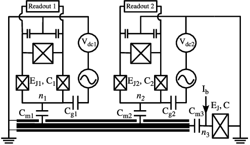
Although many of the results derived in this paper are rather general (once the Hamiltonian is put into any of the forms used in this paper), it is useful to start by analyzing a concrete superconducting quantum circuit, which will serve as our workhorse. Consider a system of two coupled charge qubits, irradiated with monochromatic off-resonance microwave fields. The circuit is shown in Fig. 1. Two split single Cooper pair box (SCB) qubits are capacitively coupled to the center conductor of a coplanar waveguide resonator. Each box has its own read-out circuitry (such as a large current-biased Josephson junction, as in the case of charge-flux qubits).
Refer to caption
Figure 1: Schematic circuit of our model system.

To ensure first-order insensitivity to charge fluctuations, we voltage-bias the gates of the SCBs at the optimal points

Cg​1​Vdc1=Cg​2​Vdc2=−e.C_{g1}V_{\mathrm{dc}1}=C_{g2}V_{\mathrm{dc}2}=-e. (1)

When two microwave fields with the same angular frequency ωd\omega_{d} and different phases ϕ1,2\phi_{1,2} are applied, the gate voltages of the SCBs have AC components

Vac1,2=Vμ​w1,2​(t)​cos⁡(ωd​t+ϕ1,2).V_{\mathrm{ac}1,2}=V_{\mathrm{\mu w}1,2}(t)\cos(\omega_{d}t+\phi_{1,2}). (2)

Written in the eigenbasis of each SCB |↑⟩=(|0⟩+|1⟩)/2|\uparrow\rangle=(|0\rangle+|1\rangle)/\sqrt{2} and |↓⟩=(|0⟩−|1⟩)/2|\downarrow\rangle=(|0\rangle-|1\rangle)/\sqrt{2}, |0⟩|0\rangle and |1⟩|1\rangle denoting two lowest charge states, the Hamiltonian has the following form (see Appendix A)

HSCB=∑j=1,2[−EJ​j2​σjz+EC​j​wj​(t)​cos⁡(ωd​t+ϕj)​σjx],H_{\mathrm{SCB}}=\sum_{j=1,2}\left[-\frac{E_{Jj}}{2}\sigma_{j}^{z}+E_{Cj}w_{j}(t)\cos(\omega_{d}t+\phi_{j})\sigma_{j}^{x}\right], (3)

where EJ​jE_{Jj} and EC​jE_{Cj} indicate the standard Josephson and charging energies, and wj(t)≡−Cg​jVμ​w​j(t)/2ew_{j}(t)\equiv-C_{gj}V_{\mathrm{\mu w}j}(t)/2e.

A large current-biased Josephson junction (CBJJ) is also coupled to the end of the resonator through a capacitor; the bias current IbI_{b} is such that, during many of the qubit operations described in this paper, only two bound states (of energy difference ω10\omega_{10} close to that of the resonator) are relevant. This junction will serve as a detector of the state of the resonator, as we will see in Sec. VI. The Hamiltonian of the CBJJ assumes the form of a two-level system,

HCBJJ=−ω102​σ3z,H_{\mathrm{CBJJ}}=-\frac{\omega_{10}}{2}\sigma_{3}^{z}, (4)

where ω10\omega_{10} denotes the transition frequency between the two lowest levels in the tilted cosine potential.

To simplify the equations, from now on our units will be such that ℏ=1\hbar=1.

Depending on the length of the stripline, the qubit-qubit and qubit-CBJJ couplings must be treated in different ways. For a relatively long resonator, the couplings are mediated by excitations in the resonator. As derived in Appendix A, the total Hamiltonian in this case is

Htot1\displaystyle H_{\mathrm{tot1}} =\displaystyle= HSCB+HCBJJ+ωr​(a†​a+1/2)\displaystyle H_{\mathrm{SCB}}+H_{\mathrm{CBJJ}}+\omega_{r}(a^{\dagger}a+1/2) (5)
+i∑j=1,2gj[σjx+2wj(t)cos(ωdt+ϕj)](a†−a)\displaystyle+i\sum_{j=1,2}g_{j}\left[\sigma_{j}^{x}+2w_{j}(t)\cos(\omega_{d}t+\phi_{j})\right](a^{\dagger}-a)
+κ⁡(σ3+−σ3−)​(a†−a),\displaystyle+\kappa(\sigma_{3}^{+}-\sigma_{3}^{-})(a^{\dagger}-a),

with ωr\omega_{r} the resonance frequency of the resonator, a†a^{\dagger} (aa) the photon creation (annihilation) operator, gjg_{j} (κ\kappa) the qubit-resonator (CBJJ-resonator) coupling strength, and σ3+\sigma_{3}^{+} (σ3−\sigma_{3}^{-}) the CBJJ raising (lowering) operator. By performing a RWA to neglect fast oscillating terms, we have

Htot1\displaystyle H_{\mathrm{tot1}} ≈\displaystyle\approx HSCB+HCBJJ+ωr​(a†​a+1/2)\displaystyle H_{\mathrm{SCB}}+H_{\mathrm{CBJJ}}+\omega_{r}(a^{\dagger}a+1/2) (6)
+i∑j=1,2gj(σj−a†−σj+a)\displaystyle+i\sum_{j=1,2}g_{j}(\sigma_{j}^{-}a^{\dagger}-\sigma_{j}^{+}a)
−κ⁡(σ3+​a+σ3−​a†),\displaystyle-\kappa(\sigma_{3}^{+}a+\sigma_{3}^{-}a^{\dagger}),

where σj+=|↓⟩​⟨↑|\sigma_{j}^{+}=|\downarrow\rangle\langle\uparrow| and σj−=|↑⟩​⟨↓|\sigma_{j}^{-}=|\uparrow\rangle\langle\downarrow| denote qubit raising and lowering operators, respectively. Here we have neglected the terms describing interactions between the qubit driving fields and the resonator (in the second line of Eq. (5)). This is justified by the fact that Rabi frequencies satisfy Ωj​(t)≡EC​j​wj​(t)≪EJ​j\Omega_{j}(t)\equiv E_{Cj}w_{j}(t)\ll E_{Jj}, and the SCBs are working in the charge regime EC​j≫EJ​jE_{Cj}\gg E_{Jj}, therefore wj​(t)w_{j}(t) should be much smaller than unity.

Long resonator limit

In the long resonator limit (the resonator length of the same order as the wavelength corresponding to an excitation with energy of the order of qubit energy), a fixed linear qubit-qubit coupling can be achieved in the dispersive regime, gj≪Δj≡ωr−EJ​jg_{j}\ll\Delta_{j}\equiv\omega_{r}-E_{Jj}. By performing a generalized Schrieffer-Wolff transformation (see Appendix C)

eA\displaystyle e^{A} =\displaystyle= exp[−i∑j=1,2gjΔj(a†σj−+aσj+)\displaystyle\exp\left[-i\sum_{j=1,2}\frac{g_{j}}{\Delta_{j}}(a^{\dagger}\sigma_{j}^{-}+a\sigma_{j}^{+})\right.
−i∑j=1,2gj​Ωj​(t)​cos⁡(ωd​t+ϕj)Δj​ωrσjz(a†+a)]\displaystyle\left.\ \ \ \ \ \ \ -i\sum_{j=1,2}\frac{g_{j}\Omega_{j}(t)\cos(\omega_{d}t+\phi_{j})}{\Delta_{j}\omega_{r}}\sigma_{j}^{z}(a^{\dagger}+a)\right]

on the Hamiltonian (6), we obtain

H~tot1\displaystyle\widetilde{H}_{\mathrm{tot1}} ≈\displaystyle\approx ∑j=1,2[−EJ​j2​σjz+Ωj​cos⁡(ωd​t+ϕj)​σjx]\displaystyle\sum_{j=1,2}\left[-\frac{E_{Jj}}{2}\sigma_{j}^{z}+\Omega_{j}\cos(\omega_{d}t+\phi_{j})\sigma_{j}^{x}\right] (7)
−g1​g2​(Δ1+Δ2)2​Δ1​Δ2​(σ1+​σ2−+σ1−​σ2+).\displaystyle-\frac{g_{1}g_{2}(\Delta_{1}+\Delta_{2})}{2\Delta_{1}\Delta_{2}}(\sigma_{1}^{+}\sigma_{2}^{-}+\sigma_{1}^{-}\sigma_{2}^{+}).

Here we assume that the CBJJ is biased far off resonance with the resonator such that it is effectively decoupled from it.

Short resonator limit

For a very short resonator (the resonator length much smaller than the wavelength corresponding to an excitation with energy of the order of qubit energy), the center conductor can be considered as a small metallic island. The two qubits and the CBJJ are capacitively coupled to this island. In Appendix B we show that the total Hamiltonian has the form

Htot2\displaystyle H_{\mathrm{tot2}} =\displaystyle= HSCB+HCBJJ+E124​σ1x​σ2x−∑j=1,2γj2​σjx​σ3y\displaystyle H_{\mathrm{SCB}}+H_{\mathrm{CBJJ}}+\frac{E_{12}}{4}\sigma_{1}^{x}\sigma_{2}^{x}-\sum_{j=1,2}\frac{\gamma_{j}}{2}\sigma_{j}^{x}\sigma_{3}^{y} (8)
+E122[w2(t)cos(ωdt+ϕ2)σ1x\displaystyle+\frac{E_{12}}{2}[w_{2}(t)\cos(\omega_{d}t+\phi_{2})\sigma_{1}^{x}
+w1(t)cos(ωdt+ϕ1)σ2x]\displaystyle\ \ \ \ \ \ \ \ \ +w_{1}(t)\cos(\omega_{d}t+\phi_{1})\sigma_{2}^{x}]
−∑j=1,2γjwj(j)cos(ωdt+ϕj)σ3y,\displaystyle-\sum_{j=1,2}\gamma_{j}w_{j}(j)\cos(\omega_{d}t+\phi_{j})\sigma_{3}^{y},

with E12/4E_{12}/4 and γj/2\gamma_{j}/2 the qubit-qubit and qubit-CBJJ coupling strengths, respectively. Due to small coupling E12≪EC​1,2E_{12}\ll E_{C1,2}, the crosstalk [12] terms in the second and third lines of Eq. (8) are negligible. We can also drop the interactions between the qubit driving fields and the CBJJ, described by the last line in Eq. (8), because wjw_{j} is small. Therefore the total Hamiltonian is approximately

Htot2≈HSCB+HCBJJ+E124​σ1x​σ2x−∑j=1,2γj2​σjx​σ3y.H_{\mathrm{tot2}}\approx H_{\mathrm{SCB}}+H_{\mathrm{CBJJ}}+\frac{E_{12}}{4}\sigma_{1}^{x}\sigma_{2}^{x}-\sum_{j=1,2}\frac{\gamma_{j}}{2}\sigma_{j}^{x}\sigma_{3}^{y}. (9)

If the coupling capacitances Cm​1,2≫Cm​3C_{m1,2}\gg C_{m3}, the direct coupling is dominating

Htot2\displaystyle H_{\mathrm{tot2}} ≈\displaystyle\approx ∑j=1,2[−EJ​j2​σjz+Ωj​cos⁡(ωd​t+ϕj)​σjx]\displaystyle\sum_{j=1,2}\left[-\frac{E_{Jj}}{2}\sigma_{j}^{z}+\Omega_{j}\cos(\omega_{d}t+\phi_{j})\sigma_{j}^{x}\right] (10)
+E124​σ1x​σ2x.\displaystyle+\frac{E_{12}}{4}\sigma_{1}^{x}\sigma_{2}^{x}.

For Cm​1,2≪Cm​3C_{m1,2}\ll C_{m3}, the two qubits can be coupled through virtual excitation of the CBJJ. By considering dispersive coupling γj≪Δj′≡ω10−EJ​j\gamma_{j}\ll\Delta_{j}^{\prime}\equiv\omega_{10}-E_{Jj}, the qubit-CBJJ couplings are eliminated by another Schrieffer-Wolff transformation similar to the one in long resonator case, and we obtain

H~tot2\displaystyle\widetilde{H}_{\mathrm{tot2}} ≈\displaystyle\approx ∑j=1,2[−EJ​j2​σjz+Ωj​cos⁡(ωd​t+ϕj)​σjx]\displaystyle\sum_{j=1,2}\left[-\frac{E_{Jj}}{2}\sigma_{j}^{z}+\Omega_{j}\cos(\omega_{d}t+\phi_{j})\sigma_{j}^{x}\right] (11)
−γ1​γ2​(Δ1′+Δ2′)4​Δ1′​Δ2′​(σ1+​σ2−+σ1−​σ2+).\displaystyle-\frac{\gamma_{1}\gamma_{2}(\Delta_{1}^{\prime}+\Delta_{2}^{\prime})}{4\Delta_{1}^{\prime}\Delta_{2}^{\prime}}(\sigma_{1}^{+}\sigma_{2}^{-}+\sigma_{1}^{-}\sigma_{2}^{+}).

The Hamiltonians (7) (10) and (11) are similar, therefore we will use a generic time-dependent Hamiltonian

H⁡(t)=∑j=1,2[−ωjL2​σjz+Ωj​cos⁡(ωd​t+ϕj)​σjx]+ωx​x​σ1x​σ2xH(t)=\sum_{j=1,2}\left[-\frac{\omega_{j}^{L}}{2}\sigma_{j}^{z}+\Omega_{j}\cos(\omega_{d}t+\phi_{j})\sigma_{j}^{x}\right]+\omega^{xx}\sigma_{1}^{x}\sigma_{2}^{x} (12)

to replace all of them. ωjL\omega_{j}^{L} and ωx​x\omega^{xx} denote the Larmor frequency of qubit-jj and the qubit-qubit coupling strength, respectively. As discussed in Sec. I, we are interested in the regime ωx​x≈|ω1L−ω2L|≪ω1,2L\omega^{xx}\approx|\omega_{1}^{L}-\omega_{2}^{L}|\ll\omega_{1,2}^{L}.

III Switchable coupling mechanism

Now, we start to derive an effective Hamiltonian with tunable coupling terms. In order to eliminate the explicit time dependence, we bring the Hamiltonian (12) into the rotating reference frame by transforming it with the operator

S1​(t)=exp⁡[i​ωd​t2​(σ1z+σ2z)].S_{1}(t)=\exp\left[\frac{i\omega_{d}t}{2}(\sigma_{1}^{z}+\sigma_{2}^{z})\right]. (13)

By performing a RWA to neglect oscillating terms with frequency 2​ωd2\omega_{d}, we get a time-independent effective Hamiltonian

Heff=H12+∑j=1,2Hj,H_{\mathrm{eff}}=H_{12}+\sum_{j=1,2}H_{j}, (14)

where

Hj=δj2​σjz+Ωj2​(cos⁡ϕj​σjx−sin⁡ϕj​σjy)H_{j}=\frac{\delta_{j}}{2}\sigma_{j}^{z}+\frac{\Omega_{j}}{2}(\cos\phi_{j}\sigma_{j}^{x}-\sin\phi_{j}\sigma_{j}^{y}) (15)

is the Hamiltonian for qubit-jj, and

H12=ωx​x2​(σ1x​σ2x+σ1y​σ2y)H_{12}=\frac{\omega^{xx}}{2}(\sigma_{1}^{x}\sigma_{2}^{x}+\sigma_{1}^{y}\sigma_{2}^{y}) (16)

describes the interaction between the two qubits. δj≡ωd−ωjL\delta_{j}\equiv\omega_{d}-\omega_{j}^{L} denotes the detuning between the driving frequency and the corresponding qubit Larmor frequency.

By diagonalizing the single-qubit Hamiltonians given by Eq. (15), we obtain the eigenenergies and the corresponding eigenstates of each single qubit:

E+(j)=ω~j/2,E−(j)=−ω~j/2,\displaystyle E_{+}^{(j)}=\widetilde{\omega}_{j}/2,\ \ \ \ \ \ \ \ \ \ \ \ \ \ \ \ \ \ \ \ \ E_{-}^{(j)}=-\widetilde{\omega}_{j}/2,
|+⟩(j)=cosθj2ei​ϕj/2|↑⟩+sinθj2e−iϕj/2|↓⟩,\displaystyle|+\rangle^{(j)}=\cos\frac{\theta_{j}}{2}e^{i\phi_{j}/2}|\uparrow\rangle+\sin\frac{\theta_{j}}{2}e^{-i\phi_{j}/2}|\downarrow\rangle, (17)
|−⟩(j)=−sinθj2ei​ϕj/2|↑⟩+cosθj2e−iϕj/2|↓⟩,\displaystyle|-\rangle^{(j)}=-\sin\frac{\theta_{j}}{2}e^{i\phi_{j}/2}|\uparrow\rangle+\cos\frac{\theta_{j}}{2}e^{-i\phi_{j}/2}|\downarrow\rangle,\ \ \ \ (18)

where

ω~j=δj2+Ωj2,sin⁡θj=Ωjω~j,cos⁡θj=δjω~j.\widetilde{\omega}_{j}=\sqrt{\delta_{j}^{2}+\Omega_{j}^{2}},\ \ \sin\theta_{j}=\frac{\Omega_{j}}{\widetilde{\omega}_{j}},\ \ \cos\theta_{j}=\frac{\delta_{j}}{\widetilde{\omega}_{j}}. (19)

We then project the time-independent effective Hamiltonian (14) onto the new basis of product states |++⟩|++\rangle, |+−⟩|+-\rangle, |−+⟩|-+\rangle, |−−⟩|--\rangle, and get

Heff′\displaystyle H_{\mathrm{eff}}^{\prime} =\displaystyle= ω~12​σz(1)+ω~22​σz(2)\displaystyle\frac{\widetilde{\omega}_{1}}{2}\sigma_{z}^{(1)}+\frac{\widetilde{\omega}_{2}}{2}\sigma_{z}^{(2)} (20)
+ωx​x2cosϕ{[sinθ1σz(1)+cosθ1σx(1)]\displaystyle+\frac{\omega^{xx}}{2}\cos\phi\left\{\left[\sin\theta_{1}\sigma_{z}^{(1)}+\cos\theta_{1}\sigma_{x}^{(1)}\right]\right.
×[sinθ2σz(2)+cosθ2σx(2)]+σy(1)σy(2)}\displaystyle\ \ \ \ \ \ \left.\times\left[\sin\theta_{2}\sigma_{z}^{(2)}+\cos\theta_{2}\sigma_{x}^{(2)}\right]+\sigma_{y}^{(1)}\sigma_{y}^{(2)}\right\}
+ωx​x2sinϕ{σy(1)[sinθ2σz(2)+cosθ2σx(2)]\displaystyle+\frac{\omega^{xx}}{2}\sin\phi\left\{\sigma_{y}^{(1)}\left[\sin\theta_{2}\sigma_{z}^{(2)}+\cos\theta_{2}\sigma_{x}^{(2)}\right]\right.
−[sinθ1σz(1)+cosθ1σx(1)]σy(2)},\displaystyle\ \ \ \ \ \ -\left.\left[\sin\theta_{1}\sigma_{z}^{(1)}+\cos\theta_{1}\sigma_{x}^{(1)}\right]\sigma_{y}^{(2)}\right\},

with the Pauli matrices σs(1)\sigma_{s}^{(1)} and σs(2)\sigma_{s}^{(2)} (s=x,y,zs=x,y,z) in the new basis, and the phase difference ϕ≡ϕ1−ϕ2\phi\equiv\phi_{1}-\phi_{2}.

Next we transform Heff′H_{\mathrm{eff}}^{\prime} into a new rotating frame with

S2​(t)=exp⁡{−i​t2​[ω~1​σz(1)+ω~2​σz(2)]}.S_{2}(t)=\exp\left\{\frac{-it}{2}\left[\widetilde{\omega}_{1}\sigma_{z}^{(1)}+\widetilde{\omega}_{2}\sigma_{z}^{(2)}\right]\right\}. (21)

By assuming that ω~1,2\widetilde{\omega}_{1,2} are much larger than the coupling strength ωx​x\omega^{xx}, we may perform a second RWA to neglect oscillating terms with frequencies ω~1,2\widetilde{\omega}_{1,2} and ω~1+ω~2\widetilde{\omega}_{1}+\widetilde{\omega}_{2}. The resulting Hamiltonian is

Heff′′\displaystyle H_{\mathrm{eff}}^{\prime\prime} =\displaystyle= ωx​x4cosϕ(1+cosθ1cosθ2){cos(δω~t)[σx(1)σx(2)+σy(1)σy(2)]−sin(δω~t)[σy(1)σx(2)−σx(1)σy(2)]}\displaystyle\frac{\omega^{xx}}{4}\cos\phi(1+\cos\theta_{1}\cos\theta_{2})\left\{\cos(\delta\widetilde{\omega}t)\left[\sigma_{x}^{(1)}\sigma_{x}^{(2)}+\sigma_{y}^{(1)}\sigma_{y}^{(2)}\right]-\sin(\delta\widetilde{\omega}t)\left[\sigma_{y}^{(1)}\sigma_{x}^{(2)}-\sigma_{x}^{(1)}\sigma_{y}^{(2)}\right]\right\} (22)
+ωx​x4​sin⁡ϕ⁡(cos⁡θ1+cos⁡θ2)​{sin⁡(δ​ω~​t)​[σx(1)​σx(2)+σy(1)​σy(2)]+cos⁡(δ​ω~​t)​[σy(1)​σx(2)−σx(1)​σy(2)]}\displaystyle+\frac{\omega^{xx}}{4}\sin\phi(\cos\theta_{1}+\cos\theta_{2})\left\{\sin(\delta\widetilde{\omega}t)\left[\sigma_{x}^{(1)}\sigma_{x}^{(2)}+\sigma_{y}^{(1)}\sigma_{y}^{(2)}\right]+\cos(\delta\widetilde{\omega}t)\left[\sigma_{y}^{(1)}\sigma_{x}^{(2)}-\sigma_{x}^{(1)}\sigma_{y}^{(2)}\right]\right\}
+ωx​x2cosϕsinθ1sinθ2σz(1)σz(2),\displaystyle+\frac{\omega^{xx}}{2}\cos\phi\sin\theta_{1}\sin\theta_{2}\sigma_{z}^{(1)}\sigma_{z}^{(2)},

with δ​ω~≡ω~1−ω~2\delta\widetilde{\omega}\equiv\widetilde{\omega}_{1}-\widetilde{\omega}_{2}. This effective Hamiltonian has oscillating terms. In the rest of this section, we discuss how to switch the effective coupling off in two limits with respect to the oscillation frequency δ​ω~\delta\widetilde{\omega}.

III.1 High δ​ω~\delta\widetilde{\omega}

The oscillating terms in (22) can be neglected if |δ​ω~|≫ωx​x|\delta\widetilde{\omega}|\gg\omega^{xx}. By using the definition of sin⁡θj\sin\theta_{j} in (19), the remaining effective Hamiltonian is expressed as

Heff′′=ωx​x2​cos⁡ϕ​Ω1​Ω2(δ12+Ω12)​(δ22+Ω22)​σz(1)​σz(2).H_{\mathrm{eff}}^{\prime\prime}=\frac{\omega^{xx}}{2}\cos\phi\frac{\Omega_{1}\Omega_{2}}{\sqrt{(\delta_{1}^{2}+\Omega_{1}^{2})(\delta_{2}^{2}+\Omega_{2}^{2})}}\sigma_{z}^{(1)}\sigma_{z}^{(2)}. (23)

A maximum coupling strength of about ωx​x/2\omega^{xx}/2 can be achieved when the driving frequency is in-resonance with the qubit Larmor frequencies ωd≈ω1,2L\omega_{d}\approx\omega_{1,2}^{L}, and large driving amplitudes Ω1,2≫|δ1,2|≈ωx​x\Omega_{1,2}\gg|\delta_{1,2}|\approx\omega^{xx} are applied in the meantime.

To turn the coupling off, we can switch off either Ω1\Omega_{1} or Ω2\Omega_{2}. Nevertheless, the two conditions must be satisfied: ω~1,2≫ωx​x\widetilde{\omega}_{1,2}\gg\omega^{xx} and |δ​ω~|≫ωx​x|\delta\widetilde{\omega}|\gg\omega^{xx}. Without loss of generality, we assume Ω2=0\Omega_{2}=0. The condition ω~1,2≫ωx​x\widetilde{\omega}_{1,2}\gg\omega^{xx} is fulfilled when the driving frequency is largely detuned from the qubit frequencies, δ1≈δ2≫ωx​x\delta_{1}\approx\delta_{2}\gg\omega^{xx} (assuming ωd>ω1,2L\omega_{d}>\omega_{1,2}^{L}). The second condition is fulfilled by driving the first qubit with a rather large amplitude Ω1≫2​δ1​ωx​x\Omega_{1}\gg\sqrt{2\delta_{1}\omega^{xx}}.

We notice that this decoupling mechanism can also be derived in the case of quantized driving fields: let us start with the usual Jaynes-Cummings form [13] of the Hamiltonian

H=ωd​a†​a−∑j=1,2ωjL2​σjz+ωx​x​σ1x​σ2x+g⁡(σ1+​a+σ1−​a†),H=\omega_{d}a^{\dagger}a-\sum_{j=1,2}\frac{\omega_{j}^{L}}{2}\sigma_{j}^{z}+\omega^{xx}\sigma_{1}^{x}\sigma_{2}^{x}+g(\sigma_{1}^{+}a+\sigma_{1}^{-}a^{\dagger}), (24)

and assume a dispersive coupling g≪δ1g\ll\delta_{1}. Then we perform a Schrieffer-Wolff transformation U=exp⁡[g⁡(σ1+​a−σ1−​a†)/δ1]U=\exp[g(\sigma_{1}^{+}a-\sigma_{1}^{-}a^{\dagger})/\delta_{1}] to eliminate the direct qubit-field coupling to leading order, and obtain

U†​H​U\displaystyle U^{\dagger}HU ≈\displaystyle\approx ωd​a†​a−[ω1L2+g2δ1​(a†​a+12)]​σ1z\displaystyle\omega_{d}a^{\dagger}a-\left[\frac{\omega_{1}^{L}}{2}+\frac{g^{2}}{\delta_{1}}\left(a^{\dagger}a+\frac{1}{2}\right)\right]\sigma_{1}^{z} (25)
−ω2L2​σ2z+ωx​x​σ1x​σ2x.\displaystyle-\frac{\omega_{2}^{L}}{2}\sigma_{2}^{z}+\omega^{xx}\sigma_{1}^{x}\sigma_{2}^{x}.

Due to the driving field applied on it, the Larmor frequency of qubit-1 is ac-Stark shifted by the quantity 2​g2​⟨a†​a⟩/δ12g^{2}\langle a^{\dagger}a\rangle/\delta_{1}. If the ac-Stark shift is much larger than the qubit-qubit coupling strength ωx​x\omega^{xx}, the two qubits are effectively decoupled.

III.2 Low δ​ω~\delta\widetilde{\omega}

A more general situation is when δ​ω~\delta\widetilde{\omega} is not so large, therefore the oscillating terms can not be neglected. Since we are considering a relatively small qubit-qubit detuning, it is not possible to eliminate 1+cosθ1cosθ21+\cos\theta_{1}\cos\theta_{2}, cos⁡θ1+cos⁡θ2\cos\theta_{1}+\cos\theta_{2}, sinθ1sinθ2\sin\theta_{1}\sin\theta_{2}, and satisfy ω~1,2≫ωx​x\widetilde{\omega}_{1,2}\gg\omega^{xx} at the same time. However, there is still a way to switch the coupling off. As shown in Eq. (22), terms in the first and the third lines have a common factor cos⁡ϕ\cos\phi. If the second line can be removed by setting δj\delta_{j} and Ωj\Omega_{j} to obtain

cos⁡θ1+cos⁡θ2=δ1δ12+Ω12+δ2δ22+Ω22=0,\cos\theta_{1}+\cos\theta_{2}=\frac{\delta_{1}}{\sqrt{\delta_{1}^{2}+\Omega_{1}^{2}}}+\frac{\delta_{2}}{\sqrt{\delta_{2}^{2}+\Omega_{2}^{2}}}=0, (26)

the rest of the Hamiltonian will be switchable by means of ϕ\phi. One solution of (26) is δ1=δ2=0\delta_{1}=\delta_{2}=0, which is realized only when the qubits are on resonance. For off-resonance qubits, Eq. (26) leads to

Ω1/Ω2=−δ1/δ2.\Omega_{1}/\Omega_{2}=-\delta_{1}/\delta_{2}. (27)

An extreme case is when δ​ω~=0\delta\widetilde{\omega}=0. By defining Δ≡ω1L−ω2L\Delta\equiv\omega_{1}^{L}-\omega_{2}^{L}, δ1=δ2−Δ\delta_{1}=\delta_{2}-\Delta, and using Eq. (19) we obtain the expression of the resonance condition

ω~1=ω~2⟹Ω12=Ω22+2​δ2​Δ−Δ2,\widetilde{\omega}_{1}=\widetilde{\omega}_{2}\ \Longrightarrow\ \Omega_{1}^{2}=\Omega_{2}^{2}+2\delta_{2}\Delta-\Delta^{2}, (28)

and the coupling coefficients

1+cosθ1cosθ2=2​δ22+Ω22−δ2​Δδ22+Ω22,\displaystyle 1+\cos\theta_{1}\cos\theta_{2}=\frac{2\delta_{2}^{2}+\Omega_{2}^{2}-\delta_{2}\Delta}{\delta_{2}^{2}+\Omega_{2}^{2}}, (29)
cos⁡θ1+cos⁡θ2=2​δ2−Δδ22+Ω22,\displaystyle\cos\theta_{1}+\cos\theta_{2}=\frac{2\delta_{2}-\Delta}{\sqrt{\delta_{2}^{2}+\Omega_{2}^{2}}}, (30)
sinθ1sinθ2=Ω2​Ω22+2​δ2​Δ−Δ2δ22+Ω22.\displaystyle\sin\theta_{1}\sin\theta_{2}=\frac{\Omega_{2}\sqrt{\Omega_{2}^{2}+2\delta_{2}\Delta-\Delta^{2}}}{\delta_{2}^{2}+\Omega_{2}^{2}}. (31)

To eliminate cos⁡θ1+cos⁡θ2\cos\theta_{1}+\cos\theta_{2}, we set the driving frequency ωd=(ω1L+ω2L)/2\omega_{d}=(\omega_{1}^{L}+\omega_{2}^{L})/2. The resonance condition (28), as well as the condition ω~1,2≫ωx​x\widetilde{\omega}_{1,2}\gg\omega^{xx}, becomes Ω1=Ω2≫ωx​x\Omega_{1}=\Omega_{2}\gg\omega^{xx}. Since |Δ|≈ωx​x|\Delta|\approx\omega^{xx}, the effective Hamiltonian has a rather simple form

Heff′′≈ωx​x4​cos⁡ϕ⁡[σx(1)​σx(2)+σy(1)​σy(2)+2​σz(1)​σz(2)].H_{\mathrm{eff}}^{\prime\prime}\approx\frac{\omega^{xx}}{4}\cos\phi\left[\sigma_{x}^{(1)}\sigma_{x}^{(2)}+\sigma_{y}^{(1)}\sigma_{y}^{(2)}+2\sigma_{z}^{(1)}\sigma_{z}^{(2)}\right]. (32)

Does this switching scheme work with quantized fields as well? Here we briefly notice that in this approach it is essential to operate with states of the electromagnetic field having well-defined phases; therefore this switching scheme can be implemented either with classical fields or with coherent states[13, 15]; Fock (number) states, even if they could be prepared experimentally, have fluctuating phases, therefore cannot be used.

IV Entangling properties

In order to characterize the effectiveness of the switchable coupling schemes derived in previous section, we need to determine the on/off ratio of the coupling with the original Hamiltonian (12). In this section, we will use the concurrence [16] to study the entanglement between the two qubits. The concurrence of a pure two-qubit state |ψ⟩|\psi\rangle is defined as

𝒞⁡(ψ)=|⟨ψ|σy⊗σy|ψ∗⟩|,{\cal C}(\psi)=|\langle\psi|\sigma_{y}\otimes\sigma_{y}|\psi^{*}\rangle|, (33)

where |ψ∗⟩|\psi^{*}\rangle is the complex conjugate of |ψ⟩|\psi\rangle. For a general two-qubit state |ψ⟩=cu​u|↑↑⟩+cu​d|↑↓⟩+cd​u|↓↑⟩+cd​d|↓↓⟩|\psi\rangle=c_{uu}|\uparrow\uparrow\rangle+c_{ud}|\uparrow\downarrow\rangle+c_{du}|\downarrow\uparrow\rangle+c_{dd}|\downarrow\downarrow\rangle, it is

𝒞⁡(ψ)=2​|cu​u​cd​d−cu​d​cd​u|≤1.{\cal C}(\psi)=2|c_{uu}c_{dd}-c_{ud}c_{du}|\leq 1. (34)

We define the on/off ratio of coupling as the ratio of the maximum concurrence obtained when the coupling is switched on to the maximum concurrence obtained when the coupling is effectively off.

In the lab frame, the concurrence can be calculated by numerically solving the Schrödinger equation with the time-dependent Hamiltonian (12) [17]. In the rotating frame, analytical calculations with the effective Hamiltonian (14) can be done under the circumstance that δ1\delta_{1} and δ2\delta_{2} are small. Here we only focus on the zero δ​ω~\delta\widetilde{\omega} case discussed in Sec. III.2. For the sake of simplicity, we also consider that the driving fields satisfy Ω1=Ω2≡Ω≫ωx​x\Omega_{1}=\Omega_{2}\equiv\Omega\gg\omega^{xx}, and specify our initial state to the ground state |↑↑⟩|\uparrow\uparrow\rangle.

We start by deriving the analytical expression of the concurrence. When ϕ1=ϕ2=0\phi_{1}=\phi_{2}=0, the coupling is switched on. The effective Hamiltonian (14) is approximately

Heff≈Ω2​(σ1x+σ2x)+ωx​x2​(σ1x​σ2x+σ1y​σ2y).H_{\mathrm{eff}}\approx\frac{\Omega}{2}(\sigma_{1}^{x}+\sigma_{2}^{x})+\frac{\omega^{xx}}{2}(\sigma_{1}^{x}\sigma_{2}^{x}+\sigma_{1}^{y}\sigma_{2}^{y}). (35)

It has eigenvalues λ1=0\lambda_{1}=0, λ2=−ωx​x\lambda_{2}=-\omega^{xx}, λ3,4=[ωx​x±(ωx​x)2+4​Ω2]/2\lambda_{3,4}=[\omega^{xx}\pm\sqrt{(\omega^{xx})^{2}+4\Omega^{2}}]/2, and the corresponding (unnormalized) eigenvectors [−1,0,0,1]T[-1,0,0,1]^{\mathrm{T}}, [0,−1,1,0]T[0,-1,1,0]^{\mathrm{T}}, [1,λ3,4/Ω,λ3,4/Ω,1]T[1,\lambda_{3,4}/\Omega,\lambda_{3,4}/\Omega,1]^{\mathrm{T}}, respectively. By expanding |↑↑⟩|\uparrow\uparrow\rangle in terms of the eigenvectors, we get the time-dependent state vector

|ψ⁡(t)⟩\displaystyle|\psi(t)\rangle =\displaystyle= [14(e−i​λ3​t+e−i​λ4t+2)+ωx​x4​(λ3−λ4)(e−i​λ4​t−e−i​λ3​t)]|↑↑⟩\displaystyle\left[\frac{1}{4}\left(e^{-i\lambda_{3}t}+e^{-i\lambda_{4}}t+2\right)+\frac{\omega^{xx}}{4(\lambda_{3}-\lambda_{4})}\left(e^{-i\lambda_{4}t}-e^{-i\lambda_{3}t}\right)\right]|\uparrow\uparrow\rangle (36)
−Ω2​(λ3−λ4)(e−i​λ4​t−e−i​λ3​t)(|↑↓⟩+|↓↑⟩)\displaystyle-\frac{\Omega}{2(\lambda_{3}-\lambda_{4})}\left(e^{-i\lambda_{4}t}-e^{-i\lambda_{3}t}\right)\left(|\uparrow\downarrow\rangle+|\downarrow\uparrow\rangle\right)
+[14(e−i​λ3​t+e−i​λ4t−2)+ωx​x4​(λ3−λ4)(e−i​λ4​t−e−i​λ3​t)]|↓↓⟩.\displaystyle+\left[\frac{1}{4}\left(e^{-i\lambda_{3}t}+e^{-i\lambda_{4}}t-2\right)+\frac{\omega^{xx}}{4(\lambda_{3}-\lambda_{4})}\left(e^{-i\lambda_{4}t}-e^{-i\lambda_{3}t}\right)\right]|\downarrow\downarrow\rangle.

Then the concurrence is approximately

𝒞⁡(t)≈|ei​ωx​x​t−1|/2=[1−cos⁡(ωx​x​t)]/2,{\cal C}(t)\approx|e^{i\omega^{xx}t}-1|/2=\sqrt{[1-\cos(\omega^{xx}t)]/2}, (37)

oscillating between 0 and 1 with a period of 2​π/ωx​x2\pi/\omega^{xx}.

According to (32), if we set ϕ1=π/2\phi_{1}=\pi/2 and ϕ2=0\phi_{2}=0, the coupling should be effectively switched off, whereas the effective Hamiltonian (14) in this case reads

Heff≈Ω2​(σ2x−σ1y)+ωx​x2​(σ1x​σ2x+σ1y​σ2y).H_{\mathrm{eff}}\approx\frac{\Omega}{2}(\sigma_{2}^{x}-\sigma_{1}^{y})+\frac{\omega^{xx}}{2}(\sigma_{1}^{x}\sigma_{2}^{x}+\sigma_{1}^{y}\sigma_{2}^{y}). (38)

By diagonalizing HeffH_{\mathrm{eff}} and expanding |↑↑⟩|\uparrow\uparrow\rangle with the eigenvectors again, we arrive at an analytical expression of the time-dependent concurrence as

𝒞⁡(t)≈(ωx​x)22​Ω2​|3+cos⁡(2​Ω​t)−4​cos⁡(Ω​t)|.{\cal C}(t)\approx\frac{(\omega^{xx})^{2}}{2\Omega^{2}}|3+\cos(2\Omega t)-4\cos(\Omega t)|. (39)

The maximum concurrence is about (2​ωx​x)2/Ω2(2\omega^{xx})^{2}/\Omega^{2}.

Thus, the on/off coupling ratio is approximately Ω2/(2​ωx​x)2\Omega^{2}/(2\omega^{xx})^{2}. To perform the numerical calculations, we set Ω=10​ωx​x\Omega=10\omega^{xx}, ωd=200​ωx​x\omega_{d}=200\omega^{xx}, ω1L=ωd+Δ/2\omega_{1}^{L}=\omega_{d}+\Delta/2, and ω2L=ωd−Δ/2\omega_{2}^{L}=\omega_{d}-\Delta/2 (considering Δ≪ωd\Delta\ll\omega_{d}). For a charge qubit (EC/EJ≫1E_{C}/E_{J}\gg 1), the probability of leakage to non-computational states is negligible for such a ratio of Ω/ω1,2L\Omega/\omega_{1,2}^{L} (see Appendix D).

Refer to caption
Refer to caption
Figure 2: (Color online) Time evolution of the concurrences for the input state |ψin⟩=|↑↑⟩|\psi_{\mathrm{in}}\rangle=|\uparrow\uparrow\rangle. (a) ϕ1=ϕ2=0\phi_{1}=\phi_{2}=0; (b) ϕ1=π/2\phi_{1}=\pi/2, ϕ2=0\phi_{2}=0. The solid (red) and dashed (blue) lines indicate the concurrences calculated with the time-dependent Hamiltonian (12) and the effective Hamiltonian (14), respectively. We have set Ω=10​ωx​x\Omega=10\omega^{xx}, ωd=20​Ω\omega_{d}=20\Omega, and ω1,2L=ωd±Δ/2\omega_{1,2}^{L}=\omega_{d}\pm\Delta/2.

In Fig. 2, we show the concurrences calculated with different values of Δ\Delta. The numerical results indicate that the switchable coupling scheme works well as long as Δ\Delta is not too big compared to ωx​x\omega^{xx}. An on/off coupling ratio of about 2020 can be obtained in a time duration longer than several π\pi-pulse widths. Once Δ\Delta becomes large, the on/off ratio is reduced. Furthermore, differences between the concurrences (dashed lines) calculated with the effective Hamiltonian (14) and the exact concurrences (solid lines) evaluated with the time-dependent Hamiltonian (12) start to appear. These differences imply that the counter-rotating terms neglected in the RWA leading to (14) cause effects larger than the Bloch-Siegert shift [18, 19].

In order to understand how the counter-rotating terms

Hcr\displaystyle H_{\mathrm{cr}} =\displaystyle= e2​i​ωd​t​(ωx​x​σ1+​σ2++Ω2​∑j=1,2ei​ϕj​σj+)\displaystyle e^{2i\omega_{d}t}\left(\omega^{xx}\sigma_{1}^{+}\sigma_{2}^{+}+\frac{\Omega}{2}\sum_{j=1,2}e^{i\phi_{j}}\sigma_{j}^{+}\right) (40)
+e−2​i​ωd​t​(ωx​x​σ1−​σ2−+Ω2​∑j=1,2e−i​ϕj​σj−)\displaystyle+e^{-2i\omega_{d}t}\left(\omega^{xx}\sigma_{1}^{-}\sigma_{2}^{-}+\frac{\Omega}{2}\sum_{j=1,2}e^{-i\phi_{j}}\sigma_{j}^{-}\right)\ \ \

behave, we extend the derivation of Bloch-Siegert shift for single two-level atom (see e.g. Chapter 7 of Ref. [19]), to our two-qubit system. To shorten the following discussions, we only consider ϕ1=ϕ2=0\phi_{1}=\phi_{2}=0.

The time-evolution operator generated by (12) can be expressed as

U(t)=S1(t)e−i​Heff​tT←exp[−i∫0tdτH~cr(τ)],U(t)=S_{1}(t)e^{-iH_{\mathrm{eff}}t}\overleftarrow{T}\exp\left[-i\int_{0}^{t}d\tau\widetilde{H}_{\mathrm{cr}}(\tau)\right], (41)

where S1​(t)S_{1}(t) is defined in Eq. (13), HeffH_{\mathrm{eff}} is given by (14), T←​exp⁡[⋯]\overleftarrow{T}\exp[\cdots] denotes the time-ordered exponential integration, and

H~cr​(τ)=ei​Heff​τ​Hcr​e−i​Heff​τ.\widetilde{H}_{\mathrm{cr}}(\tau)=e^{iH_{\mathrm{eff}}\tau}H_{\mathrm{cr}}e^{-iH_{\mathrm{eff}}\tau}. (42)

Because of the qubit-qubit coupling terms in HeffH_{\mathrm{eff}}, the transformation (42) is hard to perform. Due to the fact that only when δ1,2=∓Δ/2≫ωx​x\delta_{1,2}=\mp\Delta/2\gg\omega^{xx} the deviations become significant, we may ignore the coupling terms, and carry out (42) in the basis of {|++⟩,|+−⟩,|−+⟩,|−−⟩}\{|++\rangle,|+-\rangle,|-+\rangle,|--\rangle\}

H~cr​(τ)\displaystyle\widetilde{H}_{\mathrm{cr}}(\tau) ≈\displaystyle\approx exp⁡{i​τ2​[ω~1​σz(1)+ω~2​σz(2)]}​Hcr′\displaystyle\exp\left\{\frac{i\tau}{2}\left[\widetilde{\omega}_{1}\sigma_{z}^{(1)}+\widetilde{\omega}_{2}\sigma_{z}^{(2)}\right]\right\}H_{\mathrm{cr}}^{\prime} (43)
×exp⁡{−i​τ2​[ω~1​σz(1)+ω~2​σz(2)]},\displaystyle\times\exp\left\{\frac{-i\tau}{2}\left[\widetilde{\omega}_{1}\sigma_{z}^{(1)}+\widetilde{\omega}_{2}\sigma_{z}^{(2)}\right]\right\},

where ω~1=ω~2=(Δ/2)2+Ω2\widetilde{\omega}_{1}=\widetilde{\omega}_{2}=\sqrt{(\Delta/2)^{2}+\Omega^{2}}, and Hcr′H_{\mathrm{cr}}^{\prime} denotes the counter-rotating terms transformed into this basis.

Refer to caption
Figure 3: (Color online) Time evolution of concurrences under the same values of parameters as those in Fig. 2(a iv). Again, the solid (red) and dashed (blue) lines indicate the exact concurrence and the concurrence evaluated by the effective Hamiltonian with RWA. The dotted (green) line is the concurrence calculated with counter-rotating terms compensation.

We have evaluated the time-ordered exponential integration to second order. By transforming it back to the computational basis {|↑↑⟩,|↑↓⟩,|↓↑⟩,|↓↓⟩}\{|\uparrow\uparrow\rangle,|\uparrow\downarrow\rangle,|\downarrow\uparrow\rangle,|\downarrow\downarrow\rangle\}, we have obtained

T←exp[−i∫0tdτH~cr(τ)]\displaystyle\ \ \ \overleftarrow{T}\exp\left[-i\int_{0}^{t}d\tau\widetilde{H}_{\mathrm{cr}}(\tau)\right]
≈1−i​∫0td​τ​H~cr​(τ)−∫0td​τ2​∫0τ2d​τ1​H~cr​(τ2)​H~cr​(τ1)\displaystyle\approx 1-i\int_{0}^{t}d\tau\widetilde{H}_{\mathrm{cr}}(\tau)-\int_{0}^{t}d\tau_{2}\int_{0}^{\tau_{2}}d\tau_{1}\widetilde{H}_{\mathrm{cr}}(\tau_{2})\widetilde{H}_{\mathrm{cr}}(\tau_{1})
≈exp⁡{i​Ω3​tωd​ω~1​[σ1z+σ2z−Δ16​ω~1​(σ1x−σ2x)]}.\displaystyle\approx\exp\left\{\frac{i\Omega^{3}t}{\omega_{d}\widetilde{\omega}_{1}}\left[\sigma_{1}^{z}+\sigma_{2}^{z}-\frac{\Delta}{16\widetilde{\omega}_{1}}\left(\sigma_{1}^{x}-\sigma_{2}^{x}\right)\right]\right\}. (44)

This equation shows that besides the Bloch-Siegert shift in each qubit Larmor frequency, the counter-rotating terms also give rise to Rabi frequency shift proportional to Δ\Delta. As illustrated in Fig. 3, the concurrence recalculated by substituting (44) in (41) (dotted line) fits the exact concurrence (solid line) much better than the concurrence calculated barely with HeffH_{\mathrm{eff}} (dashed line).

V Implementation of quantum gates by composite pulses

We are now in the position to address the problem of implementing quantum gates. Simple rectangular driving pulses have been proved to be not satisfactory for precise manipulations [21]. It is better to adopt other pulse techniques [22] such as shaped pulses and composite pulses. In order to achieve arbitrary quantum gates with both high accuracy and high speed, we need to find a numerical approach to get the suitable pulse parameters (amplitudes, frequencies, phases and pulse durations). The idea is to find a certain functional, and to obtain the optimal pulse parameters by maximizing or minimizing this functional. In a previous work [23], we found a set of parameters to get a locally equivalent gate of CNOT by minimizing the functional |G1​(t)|2+|G2​(t)−1|2|G_{1}(t)|^{2}+|G_{2}(t)-1|^{2}, where G1G_{1} and G2G_{2} are two locally invariant functionals defined by Makhlin [24]. This method has a drawback that, when a locally equivalent gate is found, determining the two single-qubit gates which transform it into CNOT could be a difficult task. Therefore in this section, we minimize a different functional [25] which can lead us directly to the target gate we want.

We work in the rotating frame to reduce the computational complexity. Since in the preceding section we have found that the RWA broke down when Δ\Delta was large, here we assume Δ=2​ωx​x\Delta=2\omega^{xx}, and set the detunings δ1\delta_{1} and δ2\delta_{2} to be −Δ/2-\Delta/2 and Δ/2\Delta/2, respectively. The pulse duration of performing a gate, tpt_{p}, is equally divided into mm small intervals. We consider ϕ1\phi_{1} and ϕ2\phi_{2} as “global”parameters which are unchanged in the whole pulse duration. In order to avoid sharp edges as in rectangular pulses, we assume that in each time interval d​tdt the “local”pulse parameters Ω1,2\Omega_{1,2} vary linearly with time, and at t=0t=0 and t=tpt=t_{p}, Ω1,2=0\Omega_{1,2}=0. The unitary operator generated by the effective Hamiltonian (14) right after the pulses can be well approximated as

Ueff≈exp{−idtHeff[Ω1(m)+Ω1(m−1)2,Ω2(m)+Ω2(m−1)2]}⋯exp{−idtHeff[Ω1(1)+Ω1(0)2,Ω2(1)+Ω2(0)2]},\displaystyle U_{\mathrm{eff}}\approx\exp\left\{-idtH_{\mathrm{eff}}\left[\frac{\Omega_{1}^{(m)}+\Omega_{1}^{(m-1)}}{2},\frac{\Omega_{2}^{(m)}+\Omega_{2}^{(m-1)}}{2}\right]\right\}\cdots\exp\left\{-idtH_{\mathrm{eff}}\left[\frac{\Omega_{1}^{(1)}+\Omega_{1}^{(0)}}{2},\frac{\Omega_{2}^{(1)}+\Omega_{2}^{(0)}}{2}\right]\right\}, (45)

where Ω1,2(k)\Omega_{1,2}^{(k)} (k>0k>0) stand for the values of Ω1,2\Omega_{1,2} at the end of the kkth interval, and Ω1,2(0)\Omega_{1,2}^{(0)} denote Ω1,2\Omega_{1,2} at t=0t=0. The optimal ϕ1,2\phi_{1,2}, Ω1,2(k)\Omega_{1,2}^{(k)} and tpt_{p} for a target gate UU are achieved by searching for the global minimum of the error functional

ϵ=Tr⁡[(U−Ueff)†​(U−Ueff)].\epsilon=\sqrt{\mathrm{Tr}[(U-U_{\mathrm{eff}})^{\dagger}(U-U_{\mathrm{eff}})]}. (46)

V.1 Simulated annealing

Since normally ϵ\epsilon has many local minima, to avoid being trapped in a local minimum, we use the simulated annealing (SA) method [26, 27] to minimize ϵ\epsilon. It employs a random search of pulse parameters which allows changes not only decreasing the “energy”ϵ\epsilon, but also increasing it. The probability to accept a change is given by P=exp(−δϵ/T)P=\exp(-\delta\epsilon/T), where δ​ϵ=ϵafter​the​change−ϵbefore​the​change\delta\epsilon=\epsilon_{\mathrm{after\ the\ change}}-\epsilon_{\mathrm{before\ the\ change}}, and TT is a parameter acting as the system “temperature”. One can easily find that, if a change of pulse parameters decreases ϵ\epsilon, PP is always larger than unity, which means we always accept this change; if a change increases ϵ\epsilon, we still have chance to accept this change. Our algorithm is summarized as follows.

(i) Define the starting temperature Ts=−0.01/ln(0.8)T_{\mathrm{s}}=-0.01/\ln(0.8) and the halting temperature Th=−10−10/ln(0.8)T_{\mathrm{h}}=-10^{-10}/\ln(0.8) for the annealing process.

(ii) Define the boundaries of pulse parameters Ω1,2(k)∈[0,10​ωx​x]\Omega_{1,2}^{(k)}\in[0,10\omega^{xx}] and ϕ1,2∈[−π/2,π/2]\phi_{1,2}\in[-\pi/2,\pi/2].

(iii) Initialize the pulse parameters Ω1,2(k)=5​ωx​x\Omega_{1,2}^{(k)}=5\omega^{xx} and ϕ1,2=0\phi_{1,2}=0. Calculate the initial value of ϵ\epsilon with these pulse parameters. Initialize the temperature T=TsT=T_{\mathrm{s}}.

(iv) Repeat the following steps if T>ThT>T_{\mathrm{h}}:

a. randomly generate sequences of pulse parameters until all the parameters in the sequence are inside the boundaries;

b. evaluate ϵ\epsilon with the last sequence;

c. keep the resulting ϵ\epsilon and the pulse sequence with a probability P=exp(−δϵ/T)P=\exp(-\delta\epsilon/T);

d. after every 1000 successful evaluations of ϵ\epsilon, lower the temperature by 1%1\%.

We demonstrate two examples here: a π\pi-rotation of the first qubit around its XX-axis

UX1=e−iσ1xπ/2⊗I2=[00−i0000−i−i0000−i00],U_{X_{1}}=e^{-i\sigma_{1}^{x}\pi/2}\otimes I_{2}=\left[\begin{array}[]{cccc}0&0&-i&0\\ 0&0&0&-i\\ -i&0&0&0\\ 0&-i&0&0\end{array}\right], (47)

and a CNOT gate

UCNOT=e−iπ/4[1000010000010010],U_{\mathrm{CNOT}}=e^{-i\pi/4}\left[\begin{array}[]{cccc}1&0&0&0\\ 0&1&0&0\\ 0&0&0&1\\ 0&0&1&0\end{array}\right], (48)

where the factor exp(−iπ/4)\exp(-i\pi/4) is used to make UCNOT∈SU⁡(4)U_{\mathrm{CNOT}}\in\mathrm{SU}(4), since Tr⁡(Heff)=0\mathrm{Tr}(H_{\mathrm{eff}})=0.

Because of the off-resonance shaped pulses and the finite on/off coupling ratio, a pulse duration much longer than π/max⁡(Ω)=0.1​π/ωx​x\pi/\max(\Omega)=0.1\pi/\omega^{xx} was expected for X1X_{1} gate. By running our SA program numerous times, we have found it very difficult to minimize ϵ\epsilon to a satisfactory value if tp<0.4​π/ωx​xt_{p}<0.4\pi/\omega^{xx}. In Fig. 4(a), a possible control sequence of {Ω1​(t),Ω2​(t)}\{\Omega_{1}(t),\Omega_{2}(t)\} is presented. The pulse duration tp=0.4​π/ωx​xt_{p}=0.4\pi/\omega^{xx} has been divided into 10 intervals, and the optimized phases ϕ1=0\phi_{1}=0, ϕ2=−0.5​π\phi_{2}=-0.5\pi.

The minimum pulse duration for the CNOT gate we have found so far is tp=1.2​π/ωx​xt_{p}=1.2\pi/\omega^{xx}. Interestingly, it is approximately equal to the summation of the interaction cost [28] CH​(CNOT)=0.5​π/ωx​xC_{H}(\mathrm{CNOT})=0.5\pi/\omega^{xx} for our effective Hamiltonian, and durations for two single-qubit gates, which indicates that the SA program constructs the CNOT gate in a way close to a Cartan decomposition [29]. A possible sequence of {Ω1​(t),Ω2​(t)}\{\Omega_{1}(t),\Omega_{2}(t)\} is shown in Fig. 4(b). The corresponding phases ϕ1=−0.2​π\phi_{1}=-0.2\pi and ϕ2=0.07​π\phi_{2}=0.07\pi.

Refer to caption
Refer to caption
Figure 4: Possible sequences of Ω1​(t)\Omega_{1}(t) and Ω2​(t)\Omega_{2}(t) (a) for the single-qubit gate X1X_{1}, (b) for the CNOT gate.

V.2 Obtaining maximally entangled two-qubit states

Refer to caption
Figure 5: (Color online) Trajectories of the reduced density matrices in the rotating reference frame, projected onto the Bloch spheres. The blue and the red dots denote the motions of qubit-1 and qubit-2, respectively.

To get a visual picture of how these optimized driving pulses work, we perform a simulation of producing a maximally entangled two-qubit state by the CNOT gate. Suppose that initially the two qubits were in the ground state |↑↑⟩|\uparrow\uparrow\rangle and then a π/2\pi/2-rotation around YY-axis of qubit-1 has been applied; so the new input state is then

|ψin⟩=|↑⟩+|↓⟩2⊗|↑⟩,|\psi_{\mathrm{in}}\rangle=\frac{|\uparrow\rangle+|\downarrow\rangle}{\sqrt{2}}\otimes|\uparrow\rangle, (49)

as indicated with arrows in Fig. 5.

We then send the qubits through a CNOT gate, realized using the pulse sequences presented in Fig. 4(b); then the output state of the two qubits will be a Bell state [30]

|β↑⁣↑⟩=12(|↑↑⟩+|↓↓⟩).|\beta_{\uparrow\uparrow}\rangle=\frac{1}{\sqrt{2}}(|\uparrow\uparrow\rangle+|\downarrow\downarrow\rangle). (50)

The total density matrix for this system of two coupled qubits is obtained by numerically solving the Schrödinger equation with the effective Hamiltonian (14); the reduced density matrix of each single qubit is obtained by partially tracing out qubit-1 or qubit-2. Fig. 5 shows the motions of the reduced density matrices in the Bloch sphere picture. The reduced density matrices of each qubit end up in the centers of each of the spheres (corresponding to a zero Bloch vector), indicating that the two qubits are in a maximally entangled state [30].

For the total density matrix of the output state in rotating frame ρout\rho_{\mathrm{out}}, we find a state fidelity [22]

ℱ⁡(|β↑⁣↑⟩,ρout)=⟨β↑⁣↑|ρout|β↑⁣↑⟩>0.999.{\cal F}(|\beta_{\uparrow\uparrow}\rangle,\rho_{\mathrm{out}})=\sqrt{\langle\beta_{\uparrow\uparrow}|\rho_{\mathrm{out}}|\beta_{\uparrow\uparrow}\rangle}>0.999. (51)
Refer to caption
Figure 6: The fidelity loss due to uncertainty in measuring ωx​x\omega^{xx}.

V.3 Losses of gate fidelity

Now, we move back to the lab frame to evaluate the gate fidelity [31]

ℱ⁡(U)≡⟨ψin|U†​ρout​U|ψin⟩¯{\cal F}(U)\equiv\overline{\langle\psi_{\mathrm{in}}|U^{\dagger}\rho_{\mathrm{out}}U|\psi_{\mathrm{in}}\rangle} (52)

with the time-dependent Hamiltonian (12). We set ωd=200​ωx​x\omega_{d}=200\omega^{xx} and ω1,2L=ωd−δ1,2\omega_{1,2}^{L}=\omega_{d}-\delta_{1,2}, as in Sec. IV. By numerically solving the Schrödinger equation, we obtain ℱ⁡(X1)=0.9993{\cal F}(X_{1})=0.9993 and ℱ⁡(CNOT)=0.9982{\cal F}(\mathrm{CNOT})=0.9982. Such high fidelities can only be obtained in rather ideal cases, since the calculations have only taken gate errors due to the counter-rotating terms into account, and these errors are very small by choosing small qubit-qubit detuning. In practice, uncertainties in system parameters, external noises, etc. will cause extra fidelity losses.

The optimization method we have used relies on the well defined qubit parameters, such as the Larmor frequencies ω1,2L\omega_{1,2}^{L} and coupling strength ωx​x\omega^{xx}. In experiments on Josephson qubits, although the qubit parameters may be tunable due to specific designs, we still assume they are static, and the detailed knowledge of them are obtained by measurements. So, uncertainties in measurements of qubit Larmor frequencies and coupling strength will give rise to gate errors. By performing numerical simulations, we have found that, compared with ℱ⁡(CNOT){\cal F}(\mathrm{CNOT}), ℱ⁡(X1){\cal F}(X_{1}) is less sensitive to the uncertainties in qubit parameters. As shown in Fig. 6, there is nearly no loss of ℱ⁡(X1){\cal F}(X_{1}) even when the measured value of ωx​x\omega^{xx} is 90%90\% (or 110%110\%) of the exact ωx​x\omega^{xx}, whereas in order to keep high ℱ⁡(CNOT){\cal F}(\mathrm{CNOT}) (say >0.99>0.99), the uncertainty in ωx​x\omega^{xx} should not be more than 7%7\%. The data in Fig. 7 indicate that the uncertainties in measuring ω1,2L\omega_{1,2}^{L} should be controlled within 0.05%0.05\%, which is easily achievable with present-day electronics. If we consider typical charge qubits and dispersive coupling through a resonator, ω1,2L≈2​π×5\omega_{1,2}^{L}\approx 2\pi\times 5 GHz and ωx​x≈2​π×20\omega^{xx}\approx 2\pi\times 20 MHz (see [10]), the allowed uncertainties are in MHz range.

Refer to caption
Figure 7: (Color online) Loss of ℱ⁡(CNOT){\cal F}(\mathrm{CNOT}) due to the uncertainties in measuring ω1,2L\omega_{1,2}^{L}. ℱ⁡(X1){\cal F}(X_{1}) has similar features to ℱ⁡(CNOT){\cal F}(\mathrm{CNOT}), but less sensitive to the uncertainties (data not shown).

Nevertheless, the uncertainties in the driving pulses are not troublesome to the optimized gates. As shown in Sec. V.1, the required precision of pulse parameters are already low, only 0.1​ωx​x0.1\omega^{xx} for Ω1,2\Omega_{1,2} and 0.01​π0.01\pi for ϕ1,2\phi_{1,2}. To account for experimental imperfections (jitter and phase noise of the external electronics used to create the pulses), we also simulate the errors in pulses as normally distributed random numbers with relative error σ\sigma and null average, and find that if σ\sigma is smaller than 1%1\%, the loss of fidelity is negligible.

We now examine the effect of the electromagnetic degrees of freedom which inevitably couple to each of the two qubits, producing decoherence. We consider here the worst-case scenario [20], in which each qubit is coupled to a different environment, modeled by Lindblad superoperators

ℒt​j​[ρ]=Γϕ(j)2​(σjz​ρ​σjz−ρ),\displaystyle{\cal L}_{tj}[\rho]=\frac{\Gamma_{\phi}^{(j)}}{2}\left(\sigma_{j}^{z}\rho\sigma_{j}^{z}-\rho\right), (53)

and

ℒl​j​[ρ]\displaystyle{\cal L}_{lj}[\rho] =\displaystyle= Γ(j)2​(2​σj−​ρ​σj+−σj+​σj−​ρ−ρ​σj+​σj−),\displaystyle\frac{\Gamma^{(j)}}{2}\left(2\sigma_{j}^{-}\rho\sigma_{j}^{+}-\sigma_{j}^{+}\sigma_{j}^{-}\rho-\rho\sigma_{j}^{+}\sigma_{j}^{-}\right), (54)

describing longitudinal and transversal noise with decay rates Γ(j)\Gamma^{(j)} and Γϕ(j)\Gamma^{(j)}_{\phi} respectively. We evolve the system numerically under the simultaneous action of decoherence and of the pulse sequences corresponding to single gates and two-qubit gates. To simplify the presentation we take the decoherence rates of the two qubits equal, Γ(j)=Γ\Gamma^{(j)}=\Gamma, Γϕ(j)=Γϕ\Gamma^{(j)}_{\phi}=\Gamma_{\phi}, and we show the resulting fidelity loss due to decoherence in Fig. 8.

Refer to caption
Refer to caption
Figure 8: Loss of two-qubit (CNOT) fidelity ℱ⁡(CNOT){\cal F}(\mathrm{CNOT}) and single-qubit (X1X_{1}) fidelity ℱ⁡(X1){\cal F}(X_{1}) due to decoherence.

V.4 Summary

Compared to the FLICFORQ protocol developed in [11], our protocol do improve the speed of two-qubit gate, due to the fact that in our schemes the qubit-qubit coupling strength is reduced only by a factor of 2, and it still holds the advantages of FLICFORQ: no need to dc bias away from the optimal points and no need for active tunable coupling. For a relatively weak coupling mediated through cavity, ωx​x≈2​π×20\omega^{xx}\approx 2\pi\times 20 MHz, a CNOT gate can still be performed in about 30 ns. With two qubits directly coupled by a capacitor, ωx​x\omega^{xx} can be much larger, and it is only constrained by ωx​x≪Ω1,2≪ω1,2L\omega^{xx}\ll\Omega_{1,2}\ll\omega_{1,2}^{L}.

We have only demonstrated quantum gates with the switchable scheme for low δ​ω~\delta\widetilde{\omega} (see Sec. III.2), however, the numerical optimization method used in this section should be applicable also to the high δ​ω~\delta\widetilde{\omega} case (in Sec. III.1), with one more pulse parameter ωd\omega_{d} needed to be optimized. Since the high δ​ω~\delta\widetilde{\omega} scheme can be realized by single-qubit driving, there might be possible applications other than manipulating qubits, like bringing a qubit on and off resonance with a naturally-formed two level system (TLS) located in the Josephson junction barrier, as briefly discussed in Appendix E.

VI Quantum effects: QND entanglement

In the preceding sections, we considered that the coupling strengths between the qubits and the resonator are much smaller than the detunings between them. Two-qubit entanglement can be realized by using the CNOT gate. In this section, we move to the non-dispersive regime, and propose a protocol to create maximally entangled two-qubit states using a method [33] inspired from cavity QED systems.

We still bias the dc gate voltages of the qubits at charge degeneracy points. After exciting one qubit, we switch off the driving fields. The Hamiltonian of this qubit-qubit-resonator system is then

H=−∑j=1,2EJ​j2σjz+ωra†a+i∑j=1,2gj(a†σj−−aσj+).\displaystyle H=-\sum_{j=1,2}\frac{E_{Jj}}{2}\sigma_{j}^{z}+\omega_{r}a^{\dagger}a+i\sum_{j=1,2}g_{j}(a^{\dagger}\sigma_{j}^{-}-a\sigma_{j}^{+}).

By considering that the two qubits and the resonator have the same energy EJ​1=EJ​2=ωrE_{J1}=E_{J2}=\omega_{r}, the Hamiltonian projected onto the basis states |1~⟩≡|↓↑⟩⊗|0⟩p|\tilde{1}\rangle\equiv|\downarrow\uparrow\rangle\otimes|0\rangle_{\mathrm{p}}, |2~⟩≡|↑↓⟩⊗|0⟩p|\tilde{2}\rangle\equiv|\uparrow\downarrow\rangle\otimes|0\rangle_{\mathrm{p}} and |3~⟩≡|↑↑⟩⊗|1⟩p|\tilde{3}\rangle\equiv|\uparrow\uparrow\rangle\otimes|1\rangle_{\mathrm{p}}, with |0⟩p|0\rangle_{\mathrm{p}} and |1⟩p|1\rangle_{\mathrm{p}} the zero-photon and one-photon Fock states of the field in resonator, has the form

H=[00−i​g100−i​g2i​g1i​g20].H=\left[\begin{array}[]{ccc}0&0&-ig_{1}\\ 0&0&-ig_{2}\\ ig_{1}&ig_{2}&0\end{array}\right]. (55)

It has eigenvalues

λ1,2=±g12+g22,λ3=0,\lambda_{1,2}=\pm\sqrt{g_{1}^{2}+g_{2}^{2}},\ \ \ \ \lambda_{3}=0, (56)

with corresponding eigenvectors

|λ1,2⟩\displaystyle|\lambda_{1,2}\rangle =\displaystyle= ∓i2​(g12+g22)​(g1​|1~⟩+g2​|2~⟩)+12​|3~⟩,\displaystyle\mp\frac{i}{\sqrt{2(g_{1}^{2}+g_{2}^{2})}}\left(g_{1}|\tilde{1}\rangle+g_{2}|\tilde{2}\rangle\right)+\frac{1}{\sqrt{2}}|\tilde{3}\rangle,
|λ3⟩\displaystyle|\lambda_{3}\rangle =\displaystyle= 1g12+g22​(−g2​|1~⟩+g1​|2~⟩).\displaystyle\frac{1}{\sqrt{g_{1}^{2}+g_{2}^{2}}}\left(-g_{2}|\tilde{1}\rangle+g_{1}|\tilde{2}\rangle\right). (57)

For symmetric couplings g1=g2≡gg_{1}=g_{2}\equiv g, the eigenstate |λ3⟩|\lambda_{3}\rangle is a direct product of the resonator vacuum state and a maximally entangled two-qubit state.

An arbitrary initial state |ψin⟩=a1​|1~⟩+a2​|2~⟩+a3​|3~⟩|\psi_{\mathrm{in}}\rangle=a_{1}|\tilde{1}\rangle+a_{2}|\tilde{2}\rangle+a_{3}|\tilde{3}\rangle (|a1|2+|a2|2+|a3|2=1|a_{1}|^{2}+|a_{2}|^{2}+|a_{3}|^{2}=1) can be rewritten as

|ψin⟩\displaystyle|\psi_{\mathrm{in}}\rangle =\displaystyle= [i⁡(a1+a2)2+a32]​|λ1⟩−a1−a22​|λ3⟩\displaystyle\left[\frac{i(a_{1}+a_{2})}{2}+\frac{a_{3}}{\sqrt{2}}\right]|\lambda_{1}\rangle-\frac{a_{1}-a_{2}}{\sqrt{2}}|\lambda_{3}\rangle (58)
+[−i⁡(a1+a2)2+a32]​|λ2⟩,\displaystyle+\left[-\frac{i(a_{1}+a_{2})}{2}+\frac{a_{3}}{\sqrt{2}}\right]|\lambda_{2}\rangle,

and the time evolution of it

|ψ⁡(t)⟩\displaystyle|\psi(t)\rangle =\displaystyle= e−i​λ1​t​[i⁡(a1+a2)2+a32]​|λ1⟩+e−i​λ2​t​[−i⁡(a1+a2)2+a32]​|λ2⟩−e−i​λ3​t​a1−a22​|λ3⟩\displaystyle e^{-i\lambda_{1}t}\left[\frac{i(a_{1}+a_{2})}{2}+\frac{a_{3}}{\sqrt{2}}\right]|\lambda_{1}\rangle+e^{-i\lambda_{2}t}\left[-\frac{i(a_{1}+a_{2})}{2}+\frac{a_{3}}{\sqrt{2}}\right]|\lambda_{2}\rangle-e^{-i\lambda_{3}t}\frac{a_{1}-a_{2}}{\sqrt{2}}|\lambda_{3}\rangle (59)
=\displaystyle= [a1−a22+12​(a1+a22−i​a32)​e−i​2​g​t+12​(a1+a22+i​a32)​ei​2​g​t]​|1~⟩\displaystyle\left[\frac{a_{1}-a_{2}}{2}+\frac{1}{2}\left(\frac{a_{1}+a_{2}}{2}-\frac{ia_{3}}{\sqrt{2}}\right)e^{-i\sqrt{2}gt}+\frac{1}{2}\left(\frac{a_{1}+a_{2}}{2}+\frac{ia_{3}}{\sqrt{2}}\right)e^{i\sqrt{2}gt}\right]|\tilde{1}\rangle
+[a2−a12+12​(a1+a22−i​a32)​e−i​2​g​t+12​(a1+a22+i​a32)​ei​2​g​t]​|2~⟩\displaystyle+\left[\frac{a_{2}-a_{1}}{2}+\frac{1}{2}\left(\frac{a_{1}+a_{2}}{2}-\frac{ia_{3}}{\sqrt{2}}\right)e^{-i\sqrt{2}gt}+\frac{1}{2}\left(\frac{a_{1}+a_{2}}{2}+\frac{ia_{3}}{\sqrt{2}}\right)e^{i\sqrt{2}gt}\right]|\tilde{2}\rangle
+{[i⁡(a1+a2)2​2+a32]​e−i​2​g​t+[−i⁡(a1+a2)2​2+a32]​ei​2​g​t}​|3~⟩\displaystyle+\left\{\left[\frac{i(a_{1}+a_{2})}{2\sqrt{2}}+\frac{a_{3}}{2}\right]e^{-i\sqrt{2}gt}+\left[-\frac{i(a_{1}+a_{2})}{2\sqrt{2}}+\frac{a_{3}}{2}\right]e^{i\sqrt{2}gt}\right\}|\tilde{3}\rangle
≡\displaystyle\equiv c1​(t)​|1~⟩+c2​(t)​|2~⟩+c3​(t)​|3~⟩.\displaystyle c_{1}(t)|\tilde{1}\rangle+c_{2}(t)|\tilde{2}\rangle+c_{3}(t)|\tilde{3}\rangle.

The global entanglement among the two qubits and one photon can be quantified by the Q-measure [34]

Q⁡(t)=83​[|c1​(t)​c2​(t)|2+|c1​(t)​c3​(t)|2+|c2​(t)​c3​(t)|2],Q(t)=\frac{8}{3}\left[|c_{1}(t)c_{2}(t)|^{2}+|c_{1}(t)c_{3}(t)|^{2}+|c_{2}(t)c_{3}(t)|^{2}\right], (60)

which can be analytically calculated with Eq. (59). In Fig. 9, numerical calculations of the QQ value are illustrated.

Refer to caption
Figure 9: The QQ value as a function of time. The solid line is for an initial excitation in one of the qubits, and the dashed line for an initial excitation in the cavity.

Now, we consider the consequences of the fact that the resonator is lossy: we look at the case in which, by strongly outcoupling the cavity to a detector (e.g. the CBJJ of Fig. 1) the decay rate of the cavity is engineered to be much larger than the energy relaxation rate of each qubit.

By continuously monitoring the cavity in a period longer than the cavity life time but much shorter than the qubit relaxation time, we can know the state of the two qubits. If a photon is emitted out the cavity, the system collapses to the ground state |0~⟩≡|↑↑⟩⊗|0⟩p|\tilde{0}\rangle\equiv|\uparrow\uparrow\rangle\otimes|0\rangle_{\mathrm{p}}. Then we start from the beginning by re-exciting one qubit and repeating the monitoring. If no photon is detected, the system is in the eigenstate |λ3⟩|\lambda_{3}\rangle, which means a two-qubit entangled state is prepared.

Experimentally, the monitoring can be done by biasing the CBJJ to be in resonance with the resonator, |ω10−ωr|≪κ|\omega_{10}-\omega_{r}|\ll\kappa, where

κ≈ω10​Cm​322​CΣ​3​L​c~\kappa\approx\omega_{10}\sqrt{\frac{C_{m3}^{2}}{2C_{\Sigma 3}L\tilde{c}}} (61)

is the coupling strength between the CBJJ and the resonator, and the coupling has the form (see Eq. (89))

HR−C≈−κ⁡(a†​σ3−+a​σ3+).H_{\mathrm{R-C}}\approx-\kappa(a^{\dagger}\sigma_{3}^{-}+a\sigma_{3}^{+}). (62)

With an asymmetric design of the stripline resonator [35], such that the line has only one coupling capacitor Cm​3C_{m3} at one end, the total decay rate of the cavity is approximately equal to κ\kappa.

In order to make sure that the photon absorbed by the CBJJ will never go back to the cavity, the macroscopic quantum tunneling (MQT) rate Γ1\Gamma_{1} for the excited state |1⟩|1\rangle of the CBJJ should be much larger than κ\kappa [36]. Thus the barrier height U0U_{0} of the CBJJ should be close to 1.5​ω101.5\omega_{10}, as shown in Fig. 10(a). When a CBJJ is excited by absorbing a photon, it immediately switches to the dissipative branch and creates a voltage pulse which can be measured easily either directly or by the use of an additional dc Squid [37].

The MQT rate for the ground state |0⟩|0\rangle in this case can be calculated as [38]

Γ0=ωp2​π​864​π​U0ωp​exp⁡(−36​U05​ωp)≈2×10⁻⁴​ω10,\Gamma_{0}=\frac{\omega_{p}}{2\pi}\sqrt{\frac{864\pi U_{0}}{\omega_{p}}}\exp\left(-\frac{36U_{0}}{5\omega_{p}}\right)\approx 2\times 10^{-4}\omega_{10}, (63)

by assuming the plasma frequency ωp≈ω10\omega_{p}\approx\omega_{10}. The rate Γ1\Gamma_{1} is about 500 times of Γ0\Gamma_{0}.

To achieve the desired effect with good enough efficiency, the cavity decay rate κ\kappa should be in the range of Γ0≪κ≪Γ1\Gamma_{0}\ll\kappa\ll\Gamma_{1}.

Refer to caption
Figure 10: Schematic potential energy diagram of the CBJJ (phase regime).

This method is also suitable for the short resonator case. As derived in Appendix B, the Hamiltonian for the qubits-CBJJ system reads

H=−∑j=1,2EJ​j2σjz−ω102σ3z+E124σ1xσ2x−∑j=1,2γj2σjxσ3y.\displaystyle H=-\sum_{j=1,2}\frac{E_{Jj}}{2}\sigma_{j}^{z}-\frac{\omega_{10}}{2}\sigma_{3}^{z}+\frac{E_{12}}{4}\sigma_{1}^{x}\sigma_{2}^{x}-\sum_{j=1,2}\frac{\gamma_{j}}{2}\sigma_{j}^{x}\sigma_{3}^{y}.

If the coupling capacitance Cm​3≫Cm​1,2C_{m3}\gg C_{m1,2}, the direct coupling E12E_{12} between the two qubits is negligible, and the CBJJ itself acts as a lossy cavity. By biasing the CBJJ on resonance with the qubits, the Hamiltonian projected onto the states |1~⟩=|↓↑⟩⊗|0⟩|\tilde{1}\rangle=|\downarrow\uparrow\rangle\otimes|0\rangle, |2~⟩=|↑↓⟩⊗|0⟩|\tilde{2}\rangle=|\uparrow\downarrow\rangle\otimes|0\rangle and |3~⟩=|↑↑⟩⊗|1⟩|\tilde{3}\rangle=|\uparrow\uparrow\rangle\otimes|1\rangle is then

H=12​[00i​γ100i​γ2−i​γ1−i​γ20],H=\frac{1}{2}\left[\begin{array}[]{ccc}0&0&i\gamma_{1}\\ 0&0&i\gamma_{2}\\ -i\gamma_{1}&-i\gamma_{2}&0\end{array}\right], (64)

which has eigenvalues and eigenvectors similar to those in Eqs. (56) and (57).

In this case, the cavity decay rate is given by the MQT rate of the upper level Γ1\Gamma_{1}. It has to be much larger than the qubit decay rates, but not necessarily to be as large as that in the long resonator case. So we can bias the CBJJ barrier U0U_{0} to be higher than 1.5​ω101.5\omega_{10}. As illustrated in Fig. 10(b), when U0≈1.84​ω10U_{0}\approx 1.84\omega_{10}, Γ1\Gamma_{1} is approximately equal to 0.01​ω100.01\omega_{10}, which can be of the same order as the couplings γj\gamma_{j}.

To study the conditional time evolution of the system state, we introduce a non-Hermitian Hamiltonian [39]

Hcond=H−i​Γ​∑j=1,2σj+​σj−−i​Γ1​σ3+​σ3−.H_{\mathrm{cond}}=H-i\Gamma\sum_{j=1,2}\sigma_{j}^{+}\sigma_{j}^{-}-i\Gamma_{1}\sigma_{3}^{+}\sigma_{3}^{-}. (65)

Here we assume that both qubits are equally coupled to the CBJJ γ1=γ2≡γ\gamma_{1}=\gamma_{2}\equiv\gamma, and have the same relaxation rate Γ≪Γ1,γ\Gamma\ll\Gamma_{1},\ \gamma.

The eigenvalues and corresponding eigenvectors of HcondH_{\mathrm{cond}} are

λ1,2′≈−12​(i​Γ1±2​γ2−Γ12),λ3′=−i​Γ,\lambda_{1,2}^{\prime}\approx-\frac{1}{2}\left(i\Gamma_{1}\pm\sqrt{2\gamma^{2}-\Gamma_{1}^{2}}\right),\ \ \lambda_{3}^{\prime}=-i\Gamma, (66)

and

|λ1,2′⟩\displaystyle|\lambda_{1,2}^{\prime}\rangle ≈\displaystyle\approx −Γ1±i​2​γ2−Γ122​2​γ​(|1~⟩+|2~⟩)+12​|3~⟩,\displaystyle-\frac{\Gamma_{1}\pm i\sqrt{2\gamma^{2}-\Gamma_{1}^{2}}}{2\sqrt{2}\gamma}(|\tilde{1}\rangle+|\tilde{2}\rangle)+\frac{1}{\sqrt{2}}|\tilde{3}\rangle,
|λ3′⟩\displaystyle|\lambda_{3}^{\prime}\rangle =\displaystyle= −12​(|1~⟩−|2~⟩).\displaystyle-\frac{1}{\sqrt{2}}(|\tilde{1}\rangle-|\tilde{2}\rangle). (67)

For an initial state, say,

|ψ⁡(0)⟩=|1~⟩≈i​γ​(|λ1′⟩−|λ2′⟩)4​γ2−2​Γ12−|λ3′⟩2,|\psi(0)\rangle=|\tilde{1}\rangle\approx\frac{i\gamma(|\lambda_{1}^{\prime}\rangle-|\lambda_{2}^{\prime}\rangle)}{\sqrt{4\gamma^{2}-2\Gamma_{1}^{2}}}-\frac{|\lambda_{3}^{\prime}\rangle}{\sqrt{2}}, (68)

the (unnormalized) state vector at later time tt is given by

|ψ⁡(t)⟩\displaystyle|\psi(t)\rangle ≈\displaystyle\approx i​γ4​γ2−2​Γ12​(e−i​λ1′​t​|λ1′⟩−e−i​λ2′​t​|λ2′⟩)\displaystyle\frac{i\gamma}{\sqrt{4\gamma^{2}-2\Gamma_{1}^{2}}}\left(e^{-i\lambda_{1}^{\prime}t}|\lambda_{1}^{\prime}\rangle-e^{-i\lambda_{2}^{\prime}t}|\lambda_{2}^{\prime}\rangle\right) (69)
−12​e−i​λ3′​t​|λ3′⟩.\displaystyle-\frac{1}{\sqrt{2}}e^{-i\lambda_{3}^{\prime}t}|\lambda_{3}^{\prime}\rangle.
Refer to caption
Figure 11: The conditional occupation probabilities for the eigenstates |λ1,2′⟩|\lambda_{1,2}^{\prime}\rangle (the dashed line) and |λ3′⟩|\lambda_{3}^{\prime}\rangle (the solid line from HcondH_{\mathrm{cond}} and the dotted line from Eq. (70)). We have set EJ​1,2=ω10=10​GHzE_{J1,2}=\omega_{10}=10\ \mathrm{GHz}, γ1=γ2=100​MHz\gamma_{1}=\gamma_{2}=100\ \mathrm{MHz}, Γ1=50​MHz\Gamma_{1}=50\ \mathrm{MHz} and Γ=0.5​MHz\Gamma=0.5\ \mathrm{MHz}.

Thus the probability for finding the two qubits in the maximally entangled state (|↑↓⟩−|↓↑⟩)/2(|\uparrow\downarrow\rangle-|\downarrow\uparrow\rangle)/\sqrt{2}, conditioned on that no switching event has been detected, is obtained from Eq.(69) as

P⁡(t)\displaystyle P(t) ≈\displaystyle\approx |e−i​λ3′​t2|2/(|i​γ​e−i​λ1′​t4​γ2−2​Γ12|2CLOSE\displaystyle\left|\frac{e^{-i\lambda_{3}^{\prime}t}}{\sqrt{2}}\right|^{2}\left/\left(\left|\frac{i\gamma e^{-i\lambda_{1}^{\prime}t}}{\sqrt{4\gamma^{2}-2\Gamma_{1}^{2}}}\right|^{2}\right.\right. (70)
OPEN+|i​γ​e−i​λ2′​t4​γ2−2​Γ12|2+|e−i​λ3′​t2|2).\displaystyle\ \ \ \ \left.+\left|\frac{i\gamma e^{-i\lambda_{2}^{\prime}t}}{\sqrt{4\gamma^{2}-2\Gamma_{1}^{2}}}\right|^{2}+\left|\frac{e^{-i\lambda_{3}^{\prime}t}}{\sqrt{2}}\right|^{2}\right).

This expression approximately fits the numerical solution calculated by the conditional Hamiltonian in Eq. (65), as shown in Fig. 11. On a time scale Γ1−1≪t≪Γ−1\Gamma_{1}^{-1}\ll t\ll\Gamma^{-1}, the conditional probability of preparing the maximally entangled two-qubit state approaches unity.

In a real experiment the fidelity of the states prepared by this procedure will not be exactly 1, due to the detector inefficiency and to the spontaneous decay of the qubits during the time required to reach the asymptotic regime (less than 100 ns, Fig. 11). Detector efficiencies (visibilities) as large as 0.89 have been obtained recently for phase qubits [40]. The contribution of both these processes to the fidelity of the final state in the asymptotic regime can be calculated [33]. With parameters for superconducting qubits as given in Fig. 11, we estimate that the fidelity of preparing a Bell state by this procedure will be as high as 90%.

We conclude this part of the paper by pointing out that this method of producing entangled states is robust with respect to spurious excitations in the resonator [41] and that can be readily applied to existing experimental architectures such as phase qubit - resonator - phase qubit [42] without significant changes in the sample design.

VII Conclusion

We have analyzed the entangling properties of a system consisting of two superconducting qubits coupled to electromagnetic fields, both in the quantum and classical cases, and in a variety of experimental situations. Efficient decoupling of the qubits, two-qubit entanglement and high-fidelity quantum gates can be obtained in this model. We propose also a quantum nondemolition scheme for creating qubit-qubit maximally entangled states by monitoring the state of the resonator. Our calculations are not dependent on the physical realization of the qubit and the coupling, therefore most of our results can be adapted to various qubit species and coupling schemes.

VIII Acknowledgments

Discussions with J. Martinis are gratefully acknowledged. This work was supported by the Academy of Finland (Acad. Res. Fellowship 00857 and projects 7111994 and 7118122) and by Thailand’s Commision on Higher Education.

Appendix A Derivation of the Hamiltonian for a long resonator

In this appendix, we derive the Hamiltonian for the two SCB charge qubits and the CBJJ capacitively coupled to a 1D stripline resonator. We assume the length of the resonator is LL, then take c~\tilde{c} and l~\tilde{l} as the capacitance and the inductance per unit length.

We start with the classical Lagrangian of the resonator. At a point 0≤x≤L0\leq x\leq L, the local charge density qr​(x,t)q_{r}(x,t) and phase φr​(x,t)\varphi_{r}(x,t) satisfy the following relations

ϑ0​∂φr​(x,t)∂t=qr​(x,t)c~,∂qr​(x,t)∂t=ϑ0​∂2φr​(x,t)l~​∂x2,\displaystyle\frac{\vartheta_{0}\partial\varphi_{r}(x,t)}{\partial t}=\frac{q_{r}(x,t)}{\tilde{c}},\ \ \ \frac{\partial q_{r}(x,t)}{\partial t}=\frac{\vartheta_{0}\partial^{2}\varphi_{r}(x,t)}{\tilde{l}\partial x^{2}},

where ϑ0≡ℏ/2​e\vartheta_{0}\equiv\hbar/2e. The Lagrangian of the resonator can be written as

ℒR=ϑ022​∫0Ld​x​{c~​[∂φr​(x,t)∂t]2−1l~​[∂φr​(x,t)∂x]2}.{\cal L}_{\mathrm{R}}=\frac{\vartheta_{0}^{2}}{2}\int_{0}^{L}dx\left\{\tilde{c}\left[\frac{\partial\varphi_{r}(x,t)}{\partial t}\right]^{2}-\frac{1}{\tilde{l}}\left[\frac{\partial\varphi_{r}(x,t)}{\partial x}\right]^{2}\right\}. (71)

Because of the boundary conditions

∂φr​(x,t)∂x|x=0=∂φr​(x,t)∂x|x=L=0,\left.\frac{\partial\varphi_{r}(x,t)}{\partial x}\right|_{x=0}=\left.\frac{\partial\varphi_{r}(x,t)}{\partial x}\right|_{x=L}=0, (72)

φr​(x,t)\varphi_{r}(x,t) has the form φr​(t)​cos⁡(kn​x)\varphi_{r}(t)\cos(k_{n}x), with kn≡n​π/Lk_{n}\equiv n\pi/L. By adopting simplified notations φr​(t)→φr\varphi_{r}(t)\rightarrow\varphi_{r} and ∂φr​(t)/∂t→φ˙r\partial\varphi_{r}(t)/\partial t\rightarrow\dot{\varphi}_{r}, the Lagrangian can be rewritten as

ℒR\displaystyle{\cal L}_{\mathrm{R}} =\displaystyle= ϑ02​∫0Ld​x​[c~​φ˙r2​cos2⁡(kn​x)2−φr2​kn2​sin2⁡(kn​x)2​l~]\displaystyle\vartheta_{0}^{2}\int_{0}^{L}dx\left[\frac{\tilde{c}\dot{\varphi}_{r}^{2}\cos^{2}(k_{n}x)}{2}-\frac{\varphi_{r}^{2}k_{n}^{2}\sin^{2}(k_{n}x)}{2\tilde{l}}\right] (73)
=\displaystyle= 12​(L​c~2)​(ϑ0​φ˙r)2−12​(n2​π22​L​l~)​(ϑ0​φr)2.\displaystyle\frac{1}{2}\left(\frac{L\tilde{c}}{2}\right)(\vartheta_{0}\dot{\varphi}_{r})^{2}-\frac{1}{2}\left(\frac{n^{2}\pi^{2}}{2L\tilde{l}}\right)(\vartheta_{0}\varphi_{r})^{2}.

The Lagrangians of the SCBs and the CBJJ are as follows,

ℒSCB\displaystyle{\cal L}_{\mathrm{SCB}} =\displaystyle= ∑j=1,2Cj2​(ϑ0​φ˙j)2+∑j=1,2Cg​j2​(ϑ0​φ˙j+Vg​j)2\displaystyle\sum_{j=1,2}\frac{C_{j}}{2}(\vartheta_{0}\dot{\varphi}_{j})^{2}+\sum_{j=1,2}\frac{C_{gj}}{2}(\vartheta_{0}\dot{\varphi}_{j}+V_{gj})^{2} (74)
+∑j=1,2EJ​jcosφj,\displaystyle+\sum_{j=1,2}E_{Jj}\cos\varphi_{j},
ℒCBJJ\displaystyle{\cal L}_{\mathrm{CBJJ}} =\displaystyle= C2(ϑ0φ˙3)2+EJcosφ3+Ibϑ0φ3,\displaystyle\frac{C}{2}(\vartheta_{0}\dot{\varphi}_{3})^{2}+E_{J}\cos\varphi_{3}+I_{b}\vartheta_{0}\varphi_{3}, (75)

with the gate voltages Vg​j=Vdc​j+Vac​jV_{gj}=V_{\mathrm{dc}j}+V_{\mathrm{ac}j}.

By considering that the SCBs are close to the ends of the resonator x1→0,x2→Lx_{1}\rightarrow 0,\ x_{2}\rightarrow L, the CBJJ coupled to the end of the resonator x3=Lx_{3}=L, and taking the mode of the resonator n=2n=2, the Lagrangian for the couplings reads

ℒcoup\displaystyle{\cal L}_{\mathrm{coup}} =\displaystyle= ∑j=1,2,3Cm​j2​[ϑ0​φ˙r​(xj)+ϑ0​φ˙j]2\displaystyle\sum_{j=1,2,3}\frac{C_{mj}}{2}[\vartheta_{0}\dot{\varphi}_{r}(x_{j})+\vartheta_{0}\dot{\varphi}_{j}]^{2} (76)
≈\displaystyle\approx ∑j=1,2,3Cm​j2​(ϑ0​φ˙r+ϑ0​φ˙j)2.\displaystyle\sum_{j=1,2,3}\frac{C_{mj}}{2}(\vartheta_{0}\dot{\varphi}_{r}+\vartheta_{0}\dot{\varphi}_{j})^{2}.

The total Lagrangian is then

ℒ=ℒR+ℒSCB+ℒCBJJ+ℒcoup.{\cal L}={\cal L}_{\mathrm{R}}+{\cal L}_{\mathrm{SCB}}+{\cal L}_{\mathrm{CBJJ}}+{\cal L}_{\mathrm{coup}}. (77)

The conjugate charges are calculated by the Legendre transformation Qj=−2​e​nj=∂ℒ/∂(ϑ0​φ˙j)Q_{j}=-2en_{j}=\partial{\cal L}/\partial(\vartheta_{0}\dot{\varphi}_{j}) (j=r,1,2,3j=r,1,2,3), and the total Hamiltonian

H\displaystyle H =\displaystyle= ∑j=r,1,2,3Qj​ϑ0​φ˙j−ℒ\displaystyle\sum_{j=r,1,2,3}Q_{j}\vartheta_{0}\dot{\varphi}_{j}-{\cal L}
=\displaystyle= (2​e)22(CΣ​1​CΣ​2​CΣ​3Π)nr2+ℏ22​(2​e)2(2​π2L​l~)φr2+(2​e)22​CΣ​1(1+Cm​12​CΣ​2​CΣ​3Π)(n1−ng​1)2−EJ​1cosφ1\displaystyle\frac{(2e)^{2}}{2}\left(\frac{C_{\Sigma 1}C_{\Sigma 2}C_{\Sigma 3}}{\Pi}\right)n_{r}^{2}+\frac{\hbar^{2}}{2(2e)^{2}}\left(\frac{2\pi^{2}}{L\tilde{l}}\right)\varphi_{r}^{2}+\frac{(2e)^{2}}{2C_{\Sigma 1}}\left(1+\frac{C_{m1}^{2}C_{\Sigma 2}C_{\Sigma 3}}{\Pi}\right)(n_{1}-n_{g1})^{2}-E_{J1}\cos\varphi_{1}
+(2​e)22​CΣ​2(1+Cm​22​CΣ​1​CΣ​3Π)(n2−ng​2)2−EJ​2cosφ2+(2​e)22​CΣ​3(1+Cm​32​CΣ​1​CΣ​2Π)n32−EJcosφ3−ℏ2​eIbφ3\displaystyle+\frac{(2e)^{2}}{2C_{\Sigma 2}}\left(1+\frac{C_{m2}^{2}C_{\Sigma 1}C_{\Sigma 3}}{\Pi}\right)(n_{2}-n_{g2})^{2}-E_{J2}\cos\varphi_{2}+\frac{(2e)^{2}}{2C_{\Sigma 3}}\left(1+\frac{C_{m3}^{2}C_{\Sigma 1}C_{\Sigma 2}}{\Pi}\right)n_{3}^{2}-E_{J}\cos\varphi_{3}-\frac{\hbar}{2e}I_{b}\varphi_{3}
−(2​e)2​Cm​1​CΣ​2​CΣ​3Π​nr​(n1−ng​1)−(2​e)2​Cm​2​CΣ​1​CΣ​3Π​nr​(n2−ng​2)−(2​e)2​Cm​3​CΣ​1​CΣ​2Π​nr​n3\displaystyle-\frac{(2e)^{2}C_{m1}C_{\Sigma 2}C_{\Sigma 3}}{\Pi}n_{r}(n_{1}-n_{g1})-\frac{(2e)^{2}C_{m2}C_{\Sigma 1}C_{\Sigma 3}}{\Pi}n_{r}(n_{2}-n_{g2})-\frac{(2e)^{2}C_{m3}C_{\Sigma 1}C_{\Sigma 2}}{\Pi}n_{r}n_{3}
+(2​e)2​Cm​1​Cm​3​CΣ​2Π​(n1−ng​1)​n3+(2​e)2​Cm​2​Cm​3​CΣ​1Π​(n2−ng​2)​n3+(2​e)2​Cm​1​Cm​2​CΣ​3Π​(n1−ng​1)​(n2−ng​2),\displaystyle+\frac{(2e)^{2}C_{m1}C_{m3}C_{\Sigma 2}}{\Pi}(n_{1}-n_{g1})n_{3}+\frac{(2e)^{2}C_{m2}C_{m3}C_{\Sigma 1}}{\Pi}(n_{2}-n_{g2})n_{3}+\frac{(2e)^{2}C_{m1}C_{m2}C_{\Sigma 3}}{\Pi}(n_{1}-n_{g1})(n_{2}-n_{g2}),

where ng​j≡−Cg​jVg​j/2en_{gj}\equiv-C_{gj}V_{gj}/2e, and

Π\displaystyle\Pi ≡\displaystyle\equiv (L​c~2+CΣ​4)​CΣ​1​CΣ​2​CΣ​3−Cm​12​CΣ​2​CΣ​3\displaystyle\left(\frac{L\tilde{c}}{2}+C_{\Sigma 4}\right)C_{\Sigma 1}C_{\Sigma 2}C_{\Sigma 3}-C_{m1}^{2}C_{\Sigma 2}C_{\Sigma 3}
−Cm​22​CΣ​1​CΣ​3−Cm​32​CΣ​1​CΣ​2,\displaystyle-C_{m2}^{2}C_{\Sigma 1}C_{\Sigma 3}-C_{m3}^{2}C_{\Sigma 1}C_{\Sigma 2},

with

CΣ​1=C1+Cg​1+Cm​1,CΣ​2=C2+Cg​2+Cm​2,\displaystyle C_{\Sigma 1}=C_{1}+C_{g1}+C_{m1},\ \ \ C_{\Sigma 2}=C_{2}+C_{g2}+C_{m2},
CΣ​3=C+Cm​3,CΣ​4=Cm​1+Cm​2+Cm​3.\displaystyle C_{\Sigma 3}=C+C_{m3},\ \ \ \ \ \ \ \ \ \ C_{\Sigma 4}=C_{m1}+C_{m2}+C_{m3}.

By assuming that Cm​j≪CΣ​jC_{mj}\ll C_{\Sigma j} (j=1,2,3j=1,2,3), and defining

CΣ​r≡L​c~2+CΣ​4andLΣ​r≡L​l~2​π2\displaystyle C_{\Sigma r}\equiv\frac{L\tilde{c}}{2}+C_{\Sigma 4}\ \ \ \ \mathrm{and}\ \ \ \ L_{\Sigma r}\equiv\frac{L\tilde{l}}{2\pi^{2}}

as the effective capacitance and effective inductance of the resonator, the Hamiltonian in Eq. () can be rewritten as

H\displaystyle H ≈\displaystyle\approx (2​e)22​CΣ​r​nr2+ℏ22​(2​e)2​LΣ​r​φr2\displaystyle\frac{(2e)^{2}}{2C_{\Sigma r}}n_{r}^{2}+\frac{\hbar^{2}}{2(2e)^{2}L_{\Sigma r}}\varphi_{r}^{2} (79)
+∑j=1,2[(2​e)22​CΣ​j(nj−ng​j)2−EJ​jcosφj]\displaystyle+\sum_{j=1,2}\left[\frac{(2e)^{2}}{2C_{\Sigma j}}(n_{j}-n_{gj})^{2}-E_{Jj}\cos\varphi_{j}\right]
+(2​e)22​CΣ​3n32−EJcosφ3−ℏ2​eIbφ3\displaystyle+\frac{(2e)^{2}}{2C_{\Sigma 3}}n_{3}^{2}-E_{J}\cos\varphi_{3}-\frac{\hbar}{2e}I_{b}\varphi_{3}
−(2​e)2CΣ​r​[Cm​3CΣ​3​nr​n3+∑j=1,2Cm​jCΣ​j​nr​(nj−ng​j)]\displaystyle-\frac{(2e)^{2}}{C_{\Sigma r}}\left[\frac{C_{m3}}{C_{\Sigma 3}}n_{r}n_{3}+\sum_{j=1,2}\frac{C_{mj}}{C_{\Sigma j}}n_{r}(n_{j}-n_{gj})\right]
+(2​e)2​Cm​1​Cm​2CΣ​r​CΣ​1​CΣ​2​(n1−ng​1)​(n2−ng​2)\displaystyle+\frac{(2e)^{2}C_{m1}C_{m2}}{C_{\Sigma r}C_{\Sigma 1}C_{\Sigma 2}}(n_{1}-n_{g1})(n_{2}-n_{g2})
+(2​e)2​Cm​3CΣ​r​CΣ​3∑j=1,2Cm​jCΣ​j(nj−ng​j)n3.\displaystyle+\frac{(2e)^{2}C_{m3}}{C_{\Sigma r}C_{\Sigma 3}}\sum_{j=1,2}\frac{C_{mj}}{C_{\Sigma j}}(n_{j}-n_{gj})n_{3}.

For a relatively long resonator L​c~≫CΣ​4L\tilde{c}\gg C_{\Sigma 4}, the direct SCB-SCB and SCB-CBJJ couplings, described by the last two lines in Eq. (79), are negligible. To obtain the quantum Hamiltonian, we replace the variables nj,φjn_{j},\ \varphi_{j} by the operators n^j,φ^j\hat{n}_{j},\ \hat{\varphi}_{j} which obey the commutation relation

[φ^j,n^k]=i​δj​k,(j,k=r,1,2,3).[\hat{\varphi}_{j},\hat{n}_{k}]=i\delta_{jk},\ \ \ \ (j,k=r,1,2,3). (80)

The quantized Hamiltonian of the resonator is then

HR=(2​e)22​CΣ​r​n^r2+ℏ22​(2​e)2​LΣ​r​φ^r2=ℏ​ωr​(a†​a+12),H_{\mathrm{R}}=\frac{(2e)^{2}}{2C_{\Sigma r}}\hat{n}_{r}^{2}+\frac{\hbar^{2}}{2(2e)^{2}L_{\Sigma r}}\hat{\varphi}_{r}^{2}=\hbar\omega_{r}\left(a^{\dagger}a+\frac{1}{2}\right), (81)

where a†a^{\dagger} (a) is photon creation (annihilation) operator, and the resonance frequency

ωr=1/LΣ​r​CΣ​r≈2​π/L​l~​c~.\omega_{r}=1\left/\sqrt{L_{\Sigma r}C_{\Sigma r}}\right.\approx 2\pi\left/L\sqrt{\tilde{l}\tilde{c}}\right.. (82)

The dimensionless charge operator

n^r=i2​e​CΣ​r​ℏ​ωr2​(a†−a).\hat{n}_{r}=\frac{i}{2e}\sqrt{\frac{C_{\Sigma r}\hbar\omega_{r}}{2}}(a^{\dagger}-a). (83)

By projecting the Hamiltonian of SCBs onto the charge states |nj⟩|n_{j}\rangle, we can get

HSCB\displaystyle H_{\mathrm{SCB}} =\displaystyle= ∑j=1,2[(2​e)22​CΣ​j(n^j−ng​j)2−EJ​jcosφ^j]\displaystyle\sum_{j=1,2}\left[\frac{(2e)^{2}}{2C_{\Sigma j}}(\hat{n}_{j}-n_{gj})^{2}-E_{Jj}\cos\hat{\varphi}_{j}\right] (84)
=\displaystyle= ∑j=1,2{∑nj[(2​e)22​CΣ​j(nj−ngj)2|nj⟩⟨nj|\displaystyle\sum_{j=1,2}\left\{\sum_{n_{j}}\left[\frac{(2e)^{2}}{2C_{\Sigma j}}(n_{j}-n_{g_{j}})^{2}|n_{j}\rangle\langle n_{j}|\right.\right.
−EJ​j2(|nj+1⟩⟨nj|+|nj−1⟩⟨nj|)]}.\displaystyle-\left.\left.\frac{E_{Jj}}{2}(|n_{j}+1\rangle\langle n_{j}|+|n_{j}-1\rangle\langle n_{j}|)\right]\right\}.\ \ \ \ \ \ \

We also assume that the two SCBs are in charge regime, EC​1,2≡2​e2/CΣ​1,2≫EJ​1,2E_{C1,2}\equiv 2e^{2}/C_{\Sigma 1,2}\gg E_{J1,2}, so that we truncate (84) to the two lowest charge states of each SCB, and obtain the Hamiltonian

HSCB=∑j=1,2[EC​j​(ng​j−12)​σjz−EJ​j2​σjx].H_{\mathrm{SCB}}=\sum_{j=1,2}\left[E_{Cj}\left(n_{gj}-\frac{1}{2}\right)\sigma_{j}^{z}-\frac{E_{Jj}}{2}\sigma_{j}^{x}\right].\ \ \ (85)

Since the DC gate voltages are biased at the charge co-degeneracy point (1) and the AC voltages have the form in Eq. (2), by transforming the Hamiltonian (85) into the uncoupled eigenbasis {|↑↑⟩,|↑↓⟩,|↓↑⟩,|↓↓⟩}\{|\uparrow\uparrow\rangle,|\uparrow\downarrow\rangle,|\downarrow\uparrow\rangle,|\downarrow\downarrow\rangle\}, we arrive at

HSCB=∑j=1,2[EC​j​wj​(t)​cos⁡(ωd​t+ϕj)​σjx−EJ​j2​σjz],H_{\mathrm{SCB}}=\sum_{j=1,2}\left[E_{Cj}w_{j}(t)\cos(\omega_{d}t+\phi_{j})\sigma_{j}^{x}-\frac{E_{Jj}}{2}\sigma_{j}^{z}\right], (86)

where wj(t)≡−Cg​jVμ​w​j(t)/2ew_{j}(t)\equiv-C_{gj}V_{\mathrm{\mu w}j}(t)/2e.

For the CBJJ, we consider EC≡2​e2/CΣ​3≪EJE_{C}\equiv 2e^{2}/C_{\Sigma 3}\ll E_{J}. It is better to discuss it in the “position”space, where φ^3\hat{\varphi}_{3} acts as a position operator. In the bottom of one of its local minima (see Fig. 10), the tilted cosine potential is approximated by a harmonic potential. So the Hamiltonian is approximately

HCBJJ\displaystyle H_{\mathrm{CBJJ}} =\displaystyle= (2​e)22​CΣ​3n^32−EJcosφ3−ℏ2​eIbφ^3\displaystyle\frac{(2e)^{2}}{2C_{\Sigma 3}}\hat{n}_{3}^{2}-E_{J}\cos\varphi_{3}-\frac{\hbar}{2e}I_{b}\hat{\varphi}_{3} (87)
=\displaystyle= ℏ​ω102​(|1⟩​⟨1|−|0⟩​⟨0|)=−ℏ​ω102​σ3z.\displaystyle\frac{\hbar\omega_{10}}{2}(|1\rangle\langle 1|-|0\rangle\langle 0|)=-\frac{\hbar\omega_{10}}{2}\sigma_{3}^{z}.\ \ \ \

Here |0⟩|0\rangle and |1⟩|1\rangle indicate the ground and the first excited states of the CBJJ, not charge states anymore. ℏ​ω10\hbar\omega_{10} is the energy difference between the two states. The dimensionless charge is analogous to the momentum

n^3=i​ℏ​ω10​CΣ​32​(2​e)2​(σ3+−σ3−)=12​e​ℏ​ω10​CΣ​32​σ3y,\hat{n}_{3}=i\sqrt{\frac{\hbar\omega_{10}C_{\Sigma 3}}{2(2e)^{2}}}(\sigma_{3}^{+}-\sigma_{3}^{-})=\frac{1}{2e}\sqrt{\frac{\hbar\omega_{10}C_{\Sigma 3}}{2}}\sigma_{3}^{y}, (88)

with the raising operator σ3+=|1⟩​⟨0|\sigma_{3}^{+}=|1\rangle\langle 0| and the lowering operator σ3−=|0⟩​⟨1|\sigma_{3}^{-}=|0\rangle\langle 1|.

With these charge operators, we obtain the quantized Hamiltonians for resonator-CBJJ and resonator-SCB couplings from the fourth line in Eq. (79)

HR−C\displaystyle H_{\mathrm{R-C}} =\displaystyle= κ⁡(σ3+−σ3−)​(a†−a),\displaystyle\kappa(\sigma_{3}^{+}-\sigma_{3}^{-})(a^{\dagger}-a), (89)
HR−S\displaystyle H_{\mathrm{R-S}} =\displaystyle= i​∑j=1,2gj​[σjx+2​wj​(t)​cos⁡(ωd​t+ϕj)]​(a†−a),\displaystyle i\sum_{j=1,2}g_{j}\left[\sigma_{j}^{x}+2w_{j}(t)\cos(\omega_{d}t+\phi_{j})\right](a^{\dagger}-a),

where the coupling strengths

κ≈ℏ​Cm​32​2​ω10​ωrCΣ​3​L​c~,gj≈e​Cm​jCΣ​j​ℏ​ωrL​c~.\kappa\approx\frac{\hbar C_{m3}}{2}\sqrt{\frac{2\omega_{10}\omega_{r}}{C_{\Sigma 3}L\tilde{c}}},\ \ \ \ g_{j}\approx e\frac{C_{mj}}{C_{\Sigma j}}\sqrt{\frac{\hbar\omega_{r}}{L\tilde{c}}}. (91)

The total Hamiltonian is

H=HR+HSCB+HCBJJ+HR−S+HR−C.H=H_{\mathrm{R}}+H_{\mathrm{SCB}}+H_{\mathrm{CBJJ}}+H_{\mathrm{R-S}}+H_{\mathrm{R-C}}. (92)

For a very short resonator CΣ​r→CΣ​4C_{\Sigma r}\rightarrow C_{\Sigma 4} and nr→0n_{r}\rightarrow 0, the kinetic energy terms in Eq. (79) become the same as terms in Eq. (95), furthermore, ℏ​ωr\hbar\omega_{r} is much larger than the other energies in the system, therefore we can assume that the two SCBs and the CBJJ are directly coupled to each other.

Appendix B Derivation of the Hamiltonian for a short resonator

When the stripline resonator is very short, L​c~≪CΣ​4L\tilde{c}\ll C_{\Sigma 4}, the center conductor can be considered as an island. The SCBs and the CBJJ are capacitively coupled to this island. Instead of deriving the Hamiltonian from the classical Lagrangian of this circuit, here we use a relatively simpler method.

The system has four nodes. As shown in Fig. 1, the total charge on node jj (j=1,2,3j=1,2,3) is indicated by Qj=−2​e​njQ_{j}=-2en_{j} (22 for a Cooper pair). The center island acts as the fourth node, and the total charge on it is assumed to be Q4=−2​e​n4Q_{4}=-2en_{4}. Since the total charge on a node is equal to the sum of the charges on all capacitors connected to the node, by denoting the electrostatic potential of node jj as VjV_{j}, we write the charge equations for all the nodes in a matrix form, as

[Q1−Cg​1​Vg​1Q2−Cg​2​Vg​2Q3Q4]=[CΣ​100Cm​10CΣ​20Cm​200CΣ​3Cm​3Cm​1Cm​2Cm​3CΣ​4]​[V1V2V3V4].\left[\begin{array}[]{c}Q_{1}-C_{g1}V_{g1}\\ Q_{2}-C_{g2}V_{g2}\\ Q_{3}\\ Q_{4}\end{array}\right]=\left[\begin{array}[]{cccc}C_{\Sigma 1}&0&0&C_{m1}\\ 0&C_{\Sigma 2}&0&C_{m2}\\ 0&0&C_{\Sigma 3}&C_{m3}\\ C_{m1}&C_{m2}&C_{m3}&C_{\Sigma 4}\end{array}\right]\left[\begin{array}[]{c}V_{1}\\ V_{2}\\ V_{3}\\ V_{4}\end{array}\right]. (93)

The 4×44\times 4 matrix in Eq. (93) is called the capacitance matrix ℂ\mathbb{C}. The total electrostatic (kinetic) energy of the system can be calculated by using the matrix

T=12​ℚT​ℂ−1​ℚ,T=\frac{1}{2}\mathbb{Q}^{\mathrm{T}}\mathbb{C}^{-1}\mathbb{Q}, (94)

where ℚ\mathbb{Q} denotes the column vector of charges on the left-hand side of Eq. (93). By making the same assumption as in Appendix A, Cm​1,2,3≪CΣ​1,2,3C_{m1,2,3}\ll C_{\Sigma 1,2,3}, and take Q4=0Q_{4}=0, the result of Eq. (94) is

T\displaystyle T =\displaystyle= EC​1​(n1−ng​1)2+EC​2​(n2−ng​2)2+EC​n32\displaystyle E_{C1}(n_{1}-n_{g1})^{2}+E_{C2}(n_{2}-n_{g2})^{2}+E_{C}n_{3}^{2} (95)
+[E13​(n1−ng​1)+E23​(n2−ng​2)]​n3\displaystyle+[E_{13}(n_{1}-n_{g1})+E_{23}(n_{2}-n_{g2})]n_{3}
+E12​(n1−ng​1)​(n2−ng​2),\displaystyle+E_{12}(n_{1}-n_{g1})(n_{2}-n_{g2}),

with

EC​1≈2​e2/CΣ​1,E13≈(2​e)2​Cm​1​Cm​3CΣ​1​CΣ​3​CΣ​4,\displaystyle E_{C1}\approx 2e^{2}/C_{\Sigma 1},\ \ E_{13}\approx\frac{(2e)^{2}C_{m1}C_{m3}}{C_{\Sigma 1}C_{\Sigma 3}C_{\Sigma 4}},
EC​2≈2​e2/CΣ​2,E23≈(2​e)2​Cm​2​Cm​3CΣ​2​CΣ​3​CΣ​4,\displaystyle E_{C2}\approx 2e^{2}/C_{\Sigma 2},\ \ E_{23}\approx\frac{(2e)^{2}C_{m2}C_{m3}}{C_{\Sigma 2}C_{\Sigma 3}C_{\Sigma 4}},
EC≈2​e2/CΣ​3,E12≈(2​e)2​Cm​1​Cm​2CΣ​1​CΣ​2​CΣ​4.\displaystyle E_{C}\approx 2e^{2}/C_{\Sigma 3},\ \ \ E_{12}\approx\frac{(2e)^{2}C_{m1}C_{m2}}{C_{\Sigma 1}C_{\Sigma 2}C_{\Sigma 4}}. (96)

The inductive (potential) energy of the system can be expressed as

U=−EJ​1cosφ1−EJ​2cosφ2−EJcosφ3−ℏ2​eIbφ3,U=-E_{J1}\cos\varphi_{1}-E_{J2}\cos\varphi_{2}-E_{J}\cos\varphi_{3}-\frac{\hbar}{2e}I_{b}\varphi_{3}, (97)

where φj\varphi_{j} (j=1,2,3j=1,2,3) is the gauge-invariant phase difference across each Josephson junction.

The total classical Hamiltonian is H=T+UH=T+U. To derive the quantum Hamiltonian, we again replace the variables φj\varphi_{j} and njn_{j} by operators φ^j\hat{\varphi}_{j} and n^j\hat{n}_{j}.

The quantized Hamiltonians of the SCBs and the CBJJ have the same form as those in Eqs. (86) and (87). With the charge operators derived in Appendix A, the Hamiltonian for direct coupling between the two SCBs is given by

HS−S\displaystyle H_{\mathrm{S-S}} =\displaystyle= E12​(n^1−ng​1)​(n^2−ng​2)\displaystyle E_{12}(\hat{n}_{1}-n_{g1})(\hat{n}_{2}-n_{g2}) (98)
=\displaystyle= E124​σ1x​σ2x+E122​w2​(t)​cos⁡(ωd​t+ϕ2)​σ1x\displaystyle\frac{E_{12}}{4}\sigma_{1}^{x}\sigma_{2}^{x}+\frac{E_{12}}{2}w_{2}(t)\cos(\omega_{d}t+\phi_{2})\sigma_{1}^{x}
+E122​w1​(t)​cos⁡(ωd​t+ϕ1)​σ2x,\displaystyle+\frac{E_{12}}{2}w_{1}(t)\cos(\omega_{d}t+\phi_{1})\sigma_{2}^{x},

and the Hamiltonian for the couplings between the two SCBs and the CBJJ is derived from the second line in Eq. (95)

HS−C=−∑j=1,2γj[12σjxσ3y+wj(t)cos(ωdt+ϕj)σ3y],H_{\mathrm{S-C}}=-\sum_{j=1,2}\gamma_{j}\left[\frac{1}{2}\sigma_{j}^{x}\sigma_{3}^{y}+w_{j}(t)\cos(\omega_{d}t+\phi_{j})\sigma_{3}^{y}\right], (99)

where

γj=2​e​Cm​3CΣ​4​(Cm​jCΣ​j)​ℏ​ω102​CΣ​3.\gamma_{j}=2e\frac{C_{m3}}{C_{\Sigma 4}}\left(\frac{C_{mj}}{C_{\Sigma j}}\right)\sqrt{\frac{\hbar\omega_{10}}{2C_{\Sigma 3}}}. (100)

The total Hamiltonian of this system is finally

H=HSCB+HCBJJ+HS−S+HS−C.H=H_{\mathrm{SCB}}+H_{\mathrm{CBJJ}}+H_{\mathrm{S-S}}+H_{\mathrm{S-C}}. (101)

Appendix C Derivation of the effective Hamiltonian in the dispersive regime

We assume that the Rabi frequencies Ωj​(t)\Omega_{j}(t) change adiabatically with respect to the qubit (Larmor) frequency, so in the following calculations we take ∂Ωj/∂t=0\partial\Omega_{j}/\partial t=0. We use the Baker-Hausdorff formula to expand the transformation to second order

HA\displaystyle H_{\mathrm{A}} ≈\displaystyle\approx H+[H,A]+12​[[H,A],A]−i​∂A∂t\displaystyle H+[H,A]+\frac{1}{2}[[H,A],A]-i\frac{\partial A}{\partial t} (102)
≈\displaystyle\approx −∑j=1,2[EJ​j2−gj2Δj(a†a+12)]σjz\displaystyle-\sum_{j=1,2}\left[\frac{E_{Jj}}{2}-\frac{g_{j}^{2}}{\Delta_{j}}(a^{\dagger}a+\frac{1}{2})\right]\sigma_{j}^{z}
+∑j=1,2gj​ωdΔj​ωrΩjsin(ωdt+ϕj)(a†+a)σjz\displaystyle+\sum_{j=1,2}\frac{g_{j}\omega_{d}}{\Delta_{j}\omega_{r}}\Omega_{j}\sin(\omega_{d}t+\phi_{j})(a^{\dagger}+a)\sigma_{j}^{z}
+∑j=1,2Ωjcos(ωd+ϕj)σjx+ωra†a\displaystyle+\sum_{j=1,2}\Omega_{j}\cos(\omega_{d}+\phi_{j})\sigma_{j}^{x}+\omega_{r}a^{\dagger}a
−g1​g22​(1Δ1+1Δ2)​(σ1+​σ2−+σ1−​σ2+).\displaystyle-\frac{g_{1}g_{2}}{2}\left(\frac{1}{\Delta_{1}}+\frac{1}{\Delta_{2}}\right)(\sigma_{1}^{+}\sigma_{2}^{-}+\sigma_{1}^{-}\sigma_{2}^{+}).

By making an adiabatic approximation for the resonator, ⟨a†​a⟩=0\langle a^{\dagger}a\rangle=0 and ⟨a†+a⟩=1\langle a^{\dagger}+a\rangle=1, we neglect the ac-Stark shift and Lamb shift terms and the Hamiltonian of the resonator. The effective Hamiltonian can be written as

HA=HA0+HA1,\displaystyle H_{A}=H_{\mathrm{A}0}+H_{\mathrm{A}1},

where

HA​0=∑j=1,2gj​Ωj​ωdΔj​ωr​sin⁡(ωd​t+ϕj)​σjz,\displaystyle H_{A0}=\sum_{j=1,2}\frac{g_{j}\Omega_{j}\omega_{d}}{\Delta_{j}\omega_{r}}\sin(\omega_{d}t+\phi_{j})\sigma_{j}^{z}, (103)

and

HA​1\displaystyle H_{A1} =\displaystyle= ∑j=1,2[−EJ​j2​σjz+Ωj​cos⁡(ωd​t+ϕj)​σjx]\displaystyle\sum_{j=1,2}\left[-\frac{E_{Jj}}{2}\sigma_{j}^{z}+\Omega_{j}\cos(\omega_{d}t+\phi_{j})\sigma_{j}^{x}\right] (104)
−g1​g2​(Δ1+Δ2)2​Δ1​Δ2​(σ1+​σ2−+σ1−​σ2+).\displaystyle-\frac{g_{1}g_{2}(\Delta_{1}+\Delta_{2})}{2\Delta_{1}\Delta_{2}}(\sigma_{1}^{+}\sigma_{2}^{-}+\sigma_{1}^{-}\sigma_{2}^{+}).

Now we transform HA​1H_{A1} into the interaction picture

H~=ei​∫0td​t′​HA​0​(t′)HA​1e−i∫0tdt′HA​0(t′).\displaystyle\widetilde{H}=e^{i\int_{0}^{t}dt^{\prime}H_{A0}(t^{\prime})}H_{A1}e^{-i\int_{0}^{t}dt^{\prime}H_{A0}(t^{\prime})}. (105)

The raising and lowering operators become

σ~j±\displaystyle\tilde{\sigma}_{j}^{\pm} =\displaystyle= σj±​e±i​z​cos⁡(ωd​t+ϕj)\displaystyle\sigma_{j}^{\pm}e^{\pm iz\cos(\omega_{d}t+\phi_{j})} (106)
=\displaystyle= ∑n=−∞∞in​Jn​(±z)​ei​n​(ωd​t+ϕj),\displaystyle\sum_{n=-\infty}^{\infty}i^{n}J_{n}(\pm z)e^{in(\omega_{d}t+\phi_{j})},

where Jn​(±z)J_{n}(\pm z) is the nn-th order Bessel function of the first kind. Since z=gj​Ωj/(Δj​ωr)≪1z=g_{j}\Omega_{j}/(\Delta_{j}\omega_{r})\ll 1, J0​(±z)J_{0}(\pm z) is dominant. Therefore σ~j±≈σj±\tilde{\sigma}_{j}^{\pm}\approx\sigma_{j}^{\pm}, and the Hamiltonian

H~\displaystyle\widetilde{H} ≈\displaystyle\approx ∑j=1,2[−EJ​j2​σjz+Ωj​cos⁡(ωd​t+ϕj)​σjx]\displaystyle\sum_{j=1,2}\left[-\frac{E_{Jj}}{2}\sigma_{j}^{z}+\Omega_{j}\cos(\omega_{d}t+\phi_{j})\sigma_{j}^{x}\right] (107)
−g1​g2​(Δ1+Δ2)2​Δ1​Δ2​(σ1+​σ2−+σ1−​σ2+).\displaystyle-\frac{g_{1}g_{2}(\Delta_{1}+\Delta_{2})}{2\Delta_{1}\Delta_{2}}(\sigma_{1}^{+}\sigma_{2}^{-}+\sigma_{1}^{-}\sigma_{2}^{+}).

Appendix D Leakage out of the computational subspace

Here we only consider a single charge qubit with rectangular driving pulse Ω​cos⁡(ωd​t)\Omega\cos(\omega_{d}t). By considering the three lowest charge states |n⟩={|0⟩,|1⟩,|2⟩}|n\rangle=\{|0\rangle,|1\rangle,|2\rangle\}, and dc biasing to the degeneracy point, the Hamiltonian has the form

H\displaystyle H =\displaystyle= EC​(n^−ng)2−EJ​cos⁡φ^\displaystyle E_{C}(\hat{n}-n_{g})^{2}-E_{J}\cos\hat{\varphi}
=\displaystyle= [0−EJ/20−EJ/2−2​Ω​cos⁡(ωd​t)−EJ/20−EJ/22​EC−4​Ω​cos⁡(ωd​t)].\displaystyle\left[\begin{array}[]{ccc}0&-E_{J}/2&0\\ -E_{J}/2&-2\Omega\cos(\omega_{d}t)&-E_{J}/2\\ 0&-E_{J}/2&2E_{C}-4\Omega\cos(\omega_{d}t)\end{array}\right].

The leakage can be defined as the occupation probability of state |2⟩|2\rangle after certain pulse duration, averaged overall possible initial states |ψin⟩=cos⁡θ2​|0⟩+ei​ϕ​sin⁡θ2​|1⟩|\psi_{\mathrm{in}}\rangle=\cos\frac{\theta}{2}|0\rangle+e^{i\phi}\sin\frac{\theta}{2}|1\rangle. In Fig. 12, the leakage for a π\pi-pulse is plotted by numerically solving the Schrödinger equation with HH. The driving frequency is set to ωd=EJ\omega_{d}=E_{J}.

Refer to caption
Figure 12: (Color online) Leakage for a π\pi-pulse.

Appendix E Qubit-TLS system

A lot of experimental progress has been made recently on phase qubits following the realization that the dielectric insulator forming the Josephson junction contains two-level system (TLS) defects [4, 32]. These defects have been shown to have decoherence times comparable to that of the qubit, thus they can be addressed coherently (e.g. by tuning the qubit on- and off- resonance with them).

The form of the interaction Hamiltonian between the qubit and the TLS is of the type σx​σx\sigma_{x}\sigma_{x} in the case of phase qubits [32], and this coupling becomes important when Δ≡|ω1−ω2|≲ωx​x\Delta\equiv|\omega_{1}-\omega_{2}|\lesssim\omega^{xx}. Here we adopt the same notations as in Sec. III, ωx​x\omega^{xx} denotes the coupling strength between the qubit and the TLS, ω1\omega_{1} and ω2\omega_{2} are Larmor frequencies of the qubit and the TLS, respectively. By assuming that for a single qubit there is only one such TLS near it, and the TLS is weakly coupled to the driving field of the qubit, we may use the Hamiltonian in Eq. (24) to describe this qubit-TLS system, and therefore use the switchable scheme developed in Sec. III.1 to perform quantum gates with the qubit and the TLS.

References

  • [1] Y. Nakamura, Y. A. Pashkin, and J. S. Tsai, Nature, 398, 786 (1999); T. Duty, D. Gunnarsson, K. Bladh, and P. Delsing, Phys. Rev. B 69 140503(R) (2004).
  • [2] I. Chiorescu, Y. Nakamura, C. J. P. M. Harmans, and J. E. Mooij, Science 299, 1869 (2003).
  • [3] D. Vion, A. Aassime, A. Cottet, P. Joyez, H. Pothier, C. Urbina, D. Esteve and M. H. Devoret, Science, 296, 886 (2002).
  • [4] J. M. Martinis, S. Nam, J. Aumentado, and C. Urbina, Phys. Rev. Lett. 89, 117901 (2002).
  • [5] A. J. Berkeley, H. Xu, R. C. Ramos, M. A. Gubrud, F. W. Strauch, P. R. Johnson, J. R. Anderson, A. J. Dragt, C. J. Lobb, and F. C. Wellstood, Science 300, 1548 (2003).
  • [6] Yu. A. Paskin, T. Yamamoto, O. Astafiev, Y. Nakamura, D. V. Averin, and J. S. Tsai, Nature (London) 421, 823 (2003); T. Yamamoto, Yu. A. Pashkin, O. Astafiev, Y. Nakamura, and J. S. Tsai, Nature (London) 425, 941 (2003).
  • [7] Y. X. Liu, L.F. Wei, J. S. Tsai, and F. Nori in Phys. Rev. Lett. 96, 067003 (2006); P. Bertet, C. J. P. M. Harmans, and J. E. Mooij, Phys. Rev. B 73, 064512 (2006); Y.X. Liu, L. F. Wei, J. R. Johansson, J. S. Tsai, and F. Nori, Phys. Rev. B 76, 144518 (2007).
  • [8] A. O. Niskanen, K. Harabi, F. Yoshihara, Y. Nakamura, S. Lloyd, and J. S. Tsai, Science 316, 723 (2007); S. Ashhab, A. O. Niskanen, K. Harrabi, Y. Nakamura, T. Picot, P. C. de Groot, C. J. P. M. Harmans, J. E. Mooij, and F. Nori, Phys. Rev. B 77, 014510 (2008)
  • [9] A. Wallraff, D. I. Schuster, A. Blais, L. Frunzio, R.-S. Huang, J. Majer, S. Kumar, S. M. Girvin, and R. J. Schoelkopf, Nature (London) 431, 162 (2004); A. Wallraf, D. I. Schuster, A. Blais, L. Frunzio, J. Majer, M. H. Devoret, S. M. Girvin, and R. J. Schoelkopf, Phys. Rev. Lett. 95, 060501 (2005).
  • [10] A. Blais, J. Gambetta, A. Wallraff, D. I. Schuster, S. M. Girvin, M. H. Devoret, and R. J. Schoelkopf, Phys. Rev. A 75, 032329 (2007).
  • [11] C. Rigetti, A. Blais, and M. Devoret, Phys. Rev. Lett. 94, 240502 (2005).
  • [12] S. Ashhab, S. Matsuo, N. Hatakenaka, and F. Nori, Phys. Rev. B 74, 184504 (2006); S. Ashhab and F. Nori, Phys. Rev. B 76, 132513 (2007).
  • [13] W. P. Schleich, Quantum Optics in Phase Space (Wiley-VCH, Berlin, 2001).
  • [14] O. Gywat, F. Meier, D. Loss, and D. D. Awschalom, Phys. Rev. B 73, 125336 (2006).
  • [15] M. O. Scully and M. S. Zubairy, Quantum Optics (Cambridge University Press, Cambridge, 1997).
  • [16] W. K. Wootters, Phys. Rev. Lett. 80, 2245 (1998); S. Hill and W. K. Wootters, Phys. Rev. Lett. 78, 5022 (1997).
  • [17] The Schrödinger equation can be solved by MATLAB built-in ODE solvers such as ode45 and ode113 with high accuracy. We have used ode113, which is based on the Adams-Bashforth-Moulton multistep method. The relative error tolerance has been set to be 10−710^{-7}. Detailed information about the solvers is available in MATLAB Help documents, and a good introduction of the numerical methods behind these solvers can be found in Ref. [27].
  • [18] C. Cohen-Tannoudji, J. Dupont-Roc, and G. Grynberg, Atom-Photon Interactions (John Wiley, 1992).
  • [19] R. R. Puri, Mathematical Methods of Quantum Optics (Springer, Berlin, 2001).
  • [20] J. Li, K. Chalapat, and G. S. Paraoanu, arXiv:0806.3186.
  • [21] M. Steffen, J. M. Martinis, and I. L. Chuang, Phys. Rev. B 68, 224518 (2003).
  • [22] L. M. K. Vandersypen and I. L. Chuang, Rev. Mod. Phys. 76, 1037 (2004).
  • [23] G. S. Paraoanu, Phys. Rev. B 74, 140504(R) (2006).
  • [24] Y. Makhlin, Quantum Inf. Process. 1, 243 (2002).
  • [25] A. O. Niskanen, J. J. Vartiainen, and M. M. Salomaa, Phys. Rev. Lett. 90, 197901 (2003).
  • [26] S. Kirkpatrick, C. D. Gelatt Jr., and M. P. Vecchi, Science 220, 671 (1983).
  • [27] W. H. Press, S. A. Teukolsky, W. T. Vetterling, and B. P. Flannery, Numerical Recipes Third Edition (Cambridge University Press, Cambridge, 2007).
  • [28] G. Vidal, K. Hammerer, and J. I. Cirac, Phys. Rev. Lett. 88, 237902 (2002).
  • [29] UCNOT=U1​M​U2U_{\mathrm{CNOT}}=U_{1}MU_{2}, where U1,2∈SU⁡(2)⊗SU⁡(2)U_{1,2}\in\mathrm{SU}(2)\otimes\mathrm{SU}(2) are two single-qubit gates, and MM is called the locally equivalent gate of CNOT. See Refs. [24, 28].
  • [30] M. A. Nielsen and I. L. Chuang, Quantum Computation and Quantum Information (Cambridge University Press, Cambridge, 2000).
  • [31] J. F. Poyatos, J. I. Cirac, and P. Zoller, Phys. Rev. Lett. 78, 390 (1997).
  • [32] K. B. Cooper, M. Steffen, R. McDermott, R. W. Simmonds, S. Oh, D. A. Hite, D. P. Pappas, and J. M. Martinis, Phys. Rev. Lett. 93, 180401 (2004); J. M. Martinis, K. B. Cooper, R. McDermott, M. Steffen, M. Ansmann, K. D. Osborn, K. Cicak, S. Oh, D. P. Pappas, R. W. Simmonds, and C. C. Yu, Phys. Rev. Lett. 95, 210503 (2005); A. M. Zagoskin, S. Ashhab, J. R. Johansson, and F. Nori, Phys. Rev. Lett. 97, 077001 (2006).
  • [33] M. B. Plenio, S. F. Huelga, A. Beige, and P. L. Knight, Phys. Rev. A 59, 2468 (1999).
  • [34] D. A. Meyer and N. R. Wallach, J. Math. Phys. 43, 4273 (2002).
  • [35] A. A. Houck, D. I. Schuster, J. M. Gambetta, J. A. Schreier, B. R. Johnson, J. M. Chow, L. Frunzio, J. Majer, M. H. Devoret, S. M. Girvin, and R. J. Schoelkopf, Nature (London) 449, 328 (2007).
  • [36] We assume that the temperature is lower than ℏ​ω10/2​π​kB\hbar\omega_{10}/2\pi k_{B}, so that the thermal activation is neglected.
  • [37] M. H. Devoret and J. M. Martinis, Quantum Inf. Process. 3, 163 (2004); G. S. Paraoanu, Phys. Rev. B 72, 134528 (2005); G. S. Paraoanu, Phys. Rev. Lett. 97, 180406 (2006); G. S. Paraoanu, J. Low Temp. Phys. 146, 263 (2007).
  • [38] K. K. Likharev, Dynamics of Josephson Junctions and Circuits (OPA, Amsterdam, 1986).
  • [39] H. Carmichael, An Open Systems Approach to Quantum Optics (Springer-Verlag, Berlin, 1993).
  • [40] E. Lucero, M. Hofheinz, R. C. Bialczak, N. Katz, M. Neely, A. D. O’Connell, H. Wang, A. N. Cleland, and J. Martinis, Phys. Rev. Lett. 100, 247001 (2008).
  • [41] J. Li, K. Chalapat, and G. S. Paraoanu, arXiv:0806.3148.
  • [42] M. A. Sillanpää , J. I. Park, R. W. Simmonds, Nature 449, 438 (2007); J. Majer, J. M. Chow, J. M. Gambetta, Jens Koch, B. R. Johnson, J. A. Schreier, L. Frunzio, D. I. Schuster, A. A. Houck, A. Wallraff, A. Blais, M. H. Devoret, S. M. Girvin, R. J. Schoelkopf, Nature 449, 443 (2007).