跳到论文正文
W Papers独立论文阅读器 arXiv:0803.0355 论文正文 计算阅读时间 · 0%
引用这篇论文根据当前论文元数据生成,正式投稿前建议核对。


License: arXiv.org perpetual non-exclusive license
arXiv:0803.0355v2 [math.CA] 06 Dec 2012

The uniform Korn - Poincaré inequality
in thin domains
L’inégalité de Korn - Poincaré
dans les domaines minces

Marta Lewicka and Stefan Müller Address: Marta Lewicka, Department of Mathematics, Rutgers University, 110 Frelinghuysen Rd., Piscataway, NJ 08854-8019, USA Address: Stefan Müller, Hausdorff Center for Mathematics & Institute for Applied Mathematics, Bonn University, Endenicher Allee 60, D - 53115 Bonn, Germany Email address: lewicka@math.rutgers.edu, stefan.mueller@hcm.uni-bonn.de
Abstract.

On étudie l’inégalité de Korn-Poincaré:

‖u‖W1,2​(Sh)≤Ch​‖D⁡(u)‖L2​(Sh),\|u\|_{W^{1,2}(S^{h})}\leq C_{h}\|D(u)\|_{L^{2}(S^{h})},

dans les domaines ShS^{h} de type des coques d’épaisseurs d’ordre hh autour d’une hypersurface compacte sans bord et regulière SS de 𝐑n\mathbf{R}^{n}. Par D⁡(u)D(u), on réfère à la partie symétrique du gradient ∇u\nabla u et on suppose la condition au bord:

u⋅n→h=0 on ​∂Sh.u\cdot\vec{n}^{h}=0\quad\mbox{ on }\partial S^{h}.

On démontre que ChC_{h} reste uniformément borné car h→0h\to 0, pour tout champ de vecteurs dans une famille de cônes donnée (faisant un angle <π/2<\pi/2, uniforme en hh) autour du complément orthogonal des extensions de champs de vecteurs de Killing sur SS.

On montre que cette condition est optimale comme tout champ de Killling uu sur SS admet une famille d’extensions uhu^{h} sur ShS^{h} pour lesquelles le rapport ‖uh‖W1,2​(Sh)/‖D⁡(uh)‖L2​(Sh)\|u^{h}\|_{W^{1,2}(S^{h})}/\|D(u^{h})\|_{L^{2}(S^{h})} tend à l’infini comme h→0h\to 0, même si les ShS^{h} ne possèdent pas de symmetrie axiale.

Key words and phrases: 
Korn inequality, Killing vector fields, thin domains, Poincaré inequality
1991 Mathematics Subject Classification
74B05

1. Introduction

The objective of this paper is to study the Korn-Poincaré inequality:

(1.1) ‖u‖W1,2​(Sh)≤Ch​‖D⁡(u)‖L2​(Sh),\|u\|_{W^{1,2}(S^{h})}\leq C_{h}\|D(u)\|_{L^{2}(S^{h})},

under the tangential boundary conditions:

(1.2) u⋅n→h=0 on ​∂Sh,u\cdot\vec{n}^{h}=0\quad\mbox{ on }\partial S^{h},

in domains ShS^{h} that are shells of small thickness of order hh, around an arbitrary compact, boundaryless and smooth hypersurface SS in 𝐑n\mathbf{R}^{n}. By D⁡(u)=12​(∇u+(∇u)T)D(u)=\frac{1}{2}(\nabla u+(\nabla u)^{T}) we denote the symmetric part of the gradient ∇u\nabla u.

Korn’s inequality was discovered in the early X​XXXth century, in the context of the boundary value problem of linear elastostatics [15, 16]. There is by now an extensive literature on the subject, relating to various contexts and various boundary conditions (see for example a review [11], and the references therein). If (1.2) is replaced by u=0u=0 on ∂Sh\partial S^{h}, one can easily prove that ‖∇u‖L2≤2​‖D⁡(u)‖L2\|\nabla u\|_{L^{2}}\leq\sqrt{2}\|D(u)\|_{L^{2}}, and so (1.1) follows by the Poincaré inequality. In the absence of this boundary condition, or with its weaker versions, the bound (1.1) requires an extra assumption to eliminate pure rotations and translations, when D⁡(u)=0D(u)=0 but ∇u≠0\nabla u\neq 0. In particular, (1.1) holds for all W1,2​(Sh)W^{1,2}(S^{h}) vector fields uu satisfying (1.2), which are L2L^{2}- orthogonal to the space of those linear fields on ShS^{h} with skew-symmetric gradient that are themselves tangent on the boundary.

We are interested in the behaviour of the constant ChC_{h}, as h→0h\to 0. It turns out that in general, ChC_{h} may blow up, even if ShS^{h} are not rotationally symmetric (and so the aforementioned spaces are trivial). The correct way of looking at this problem is to consider the asymptotic inequality as h→0h\to 0, i.e. the related Korn inequality on SS (see also [2]):

(1.3) ‖v‖W1,2​(S)≤C​‖D⁡(v)‖L2​(S).\|v\|_{W^{1,2}(S)}\leq C\|D(v)\|_{L^{2}(S)}.

This inequality holds true for all tangent vector fields vv on SS, which are L2L^{2}-orthogonal to the space of Killing fields on SS. A Killing field vv is defined to be a smooth tangent vector field which generates a one-parameter family of isometries on SS. It is well known that the space of Killing fields on a given surface is a finite dimensional Lie algebra. An equivalent characterisation is:

(1.4) D(v)=0, i.e.: τ∇v(x)τ=0∀x∈S∀τ∈TxS.D(v)=0,\qquad\mbox{ i.e.: }\tau\nabla v(x)\tau=0\quad\forall x\in S\quad\forall\tau\in T_{x}S.

In this paper, we first notice that any vv satisfying (1.4) admits a family of extensions vh:Sh→𝐑nv^{h}:S^{h}\to\mathbf{R}^{n}, such that the boundary conditions (1.2) hold and so that the ratio ‖vh‖W1,2​(Sh)/‖D⁡(vh)‖L2​(Sh)\|v^{h}\|_{W^{1,2}(S^{h})}/\|D(v^{h})\|_{L^{2}(S^{h})} goes to infinity as h→0h\to 0. This construction turns out to be the worst case scenario for the possible blow-up of ChC_{h}. Our main results state that the constants ChC_{h} remain uniformly bounded for vector fields uu inside any family of cones (with angle <π/2<\pi/2, uniform in hh) around the orthogonal complement of the space of extensions of all Killing fields on SS.

Our main motivation in this work has been its application to dynamics of Navier-Stokes equations in thin 33-dimensional domains. Thin domains are encountered in many problems in solid or fluid mechanics. For example, in ocean dynamics, one is dealing with the fluid regions which are thin compared to the horizontal length scales. Other examples include lubrication, meteorology, blood circulation etc.; they are a part of a broader study of the behaviour of various PDEs on thin nn-dimensional domains, where n≥2n\geq 2 (for a review see [20]).

The study of the global existence and asymptotic properties of solutions to the Navier-Stokes equations in thin 33d domains began with Raugel and Sell in [21]. They proved global existence of strong solutions for large initial data and in presence of large forcing, for the sufficiently thin 33d product domain Ω=Q×(0,ϵ)\Omega=Q\times(0,\epsilon), with the boundary conditions either purely periodical or combined periodic-Dirichlet. Further generalisations to other boundary conditions followed (see the references in [12]). Towards analysing thin domains other than simple product domains, Iftimie, Raugel and Sell [12] treated domains of the type: Ω={x∈𝐑3;(x1,x2)∈Q,0<x3<ϵg(x1,x2)}\Omega=\{x\in{\mathbf{R}}^{3};~(x_{1},x_{2})\in Q,~0<x_{3}<\epsilon g(x_{1},x_{2})\}, with the mixed boundary conditions: periodic on the lateral boundary and the Navier boundary conditions:

(1.5) D(u)n→h||n→h and u⋅n→h=0 on ∂ShD(u)\vec{n}^{h}||\vec{n}^{h}\mbox{ and }u\cdot\vec{n}^{h}=0\quad\mbox{ on }\partial S^{h}

on the top and on the bottom.

The Korn inequality arises naturally when one considers the incompressible flow subject to (1.5), for the following reason. In order to define the relevant Stokes operator one uses the symmetric bilinear form B⁡(u,v)=∫D⁡(u):D⁡(v)B(u,v)=\int D(u):D(v) rather than the usual ∫∇u:∇v\int\nabla u:\nabla v. Hence the energy methods give suitable bounds for ‖D⁡(uh)‖L2​(Sh)\|D(u^{h})\|_{L^{2}(S^{h})}, for a solution flow uhu^{h} in ShS^{h}. On the other hand, in order to establish compactness in the limit problem as h→0h\to 0, one needs bounds for the W1,2W^{1,2} norm of uhu^{h}, with constants independent of hh. The inequality (1.1) (with uniform constants ChC_{h}) provides thus a necessary uniform equivalence of the two norms ‖uh‖W1,2\|u^{h}\|_{W^{1,2}} and ‖D⁡(uh)‖L2\|D(u^{h})\|_{L^{2}} on ShS^{h}.

It is therefore hoped that we can apply the result of this paper to study the dynamics of the Navier-Stokes equations, under the Navier boundary conditions, in thin shells with various geometries of the reference surface SS and of the boundaries of ShS^{h}.

Starting with the original papers of Korn [15, 16], Korn’s inequality has also been widely used as a basic tool for the existence of solutions of the linearised displacement-traction equations in elasticity [4, 3, 11]. In this context, for a given displacement vector field uu, the matrix field D⁡(u)D(u) is the linearised strain, which measures the pointwise deviation of the deformation I​d+ϵ​uId+\epsilon u from a rigid motion, up to the first order terms in ϵ\epsilon. Hence, Korn’s inequality can be interpreted as a rigidity estimate for small displacement deformations: they are W1,2W^{1,2} close to I​dId, by the error given in the right hand side of (1.1). A nonlinear version of this rigidity estimate, obtained recently in [5], has been extensively applied to problems in nonlinear elasticity and plate theories (see eg [5, 6]). Earlier, Korn’s inequalities in thin neighbourhoods of flat surfaces have been discussed in series of papers by Kohn and Vogelius [14]. They derive an estimate which degenerates as h→0h\to 0 for clamped boundary conditions at the side of the plate. An analogous result in our setting is given in Theorem 2.3.

Acknowledgments. M.L. was partially supported by the NSF grants DMS-0707275 and DMS-0846996, and by the Polish MN grant N N201 547438.

2. The main theorems

Let SS be a smooth, closed hypersurface (a compact boundaryless manifold of co-dimension 11) in 𝐑n\mathbf{R}^{n}. Consider a family {Sh}h>0\{S^{h}\}_{h>0} of thin shells around SS:

Sh={z=x+tn→(x);x∈S,−g1h(x)<t<g2h(x)},S^{h}=\{z=x+t\vec{n}(x);~x\in S,~-g_{1}^{h}(x)<t<g_{2}^{h}(x)\},

whose boundary is given by smooth positive functions g1h,g2h:S⟶𝐑g_{1}^{h},g_{2}^{h}:S\longrightarrow\mathbf{R}. We will use the following notation: n→h\vec{n}^{h} for the outward unit normal to ∂Sh\partial S^{h}, n→​(x)\vec{n}(x) for the outward unit normal to SS (seen as the boundary of some bounded domain in 𝐑n\mathbf{R}^{n}), Tx​ST_{x}S for the tangent space to SS at a given x∈Sx\in S. The projection onto SS along n→\vec{n} will be denoted by π\pi, so that, for hh sufficiently small:

π⁡(z)=x∀z=x+t​n→​(x)∈Sh.\pi(z)=x\qquad\forall z=x+t\vec{n}(x)\in S^{h}.

The standard Korn inequality (see Theorem 9.1 in Appendix A) on bounded Lipschitz domains implies that for each u∈W1,2​(Sh,𝐑n)u\in W^{1,2}(S^{h},\mathbf{R}^{n}) satisfying the orthogonality condition:

(2.1) ∫Shu⁡(z)⋅(A​z+b)​d​z=0,∀A∈s​o​(n),∀b∈𝐑n\int_{S^{h}}u(z)\cdot(Az+b)~\mbox{d}z=0,\quad\forall A\in so(n),\quad\forall b\in\mathbf{R}^{n}

one has:

(2.2) ‖u‖W1,2​(Sh)≤Ch​‖D⁡(u)‖L2​(Sh)\|u\|_{W^{1,2}(S^{h})}\leq C_{h}\|D(u)\|_{L^{2}(S^{h})}

and the constant ChC_{h} depends only on the domain ShS^{h}, but not on uu. Here, s​o​(n)so(n) stands for the linear space of all n×nn\times n skew-symmetric matrices:

so(n)={A∈Mn×n;A=−AT}={A∈Mn×n;τTAτ=0∀τ∈𝐑n}so(n)=\{A\in M^{n\times n};~A=-A^{T}\}=\{A\in M^{n\times n};~\tau^{T}A\tau=0\quad\forall\tau\in\mathbf{R}^{n}\}

while by D⁡(u)D(u) we mean the symmetric part of ∇u\nabla u:

D⁡(u)=12​(∇u+(∇u)T).D(u)=\frac{1}{2}\left(\nabla u+(\nabla u)^{T}\right).

The same result is true for uu satisfying additionally:

u⋅n→h=0​ on ​∂Sh,u\cdot\vec{n}^{h}=0~~~\mbox{ on }\partial S^{h},

when in (2.1) we take only linear fields A​z+b∈ℛ∂​(Sh)Az+b\in\mathcal{R}_{\partial}(S^{h}); with skew-symmetric gradient, and satisfying the same boundary condition as uu:

ℛ∂(Sh)={w=Az+b;A∈so(n),b∈𝐑n,w⋅n→h=0 on ∂Sh}.\mathcal{R}_{\partial}(S^{h})=\{w=Az+b;~~A\in so(n),b\in\mathbf{R}^{n},w\cdot\vec{n}^{h}=0\mbox{ on }\partial S^{h}\}.

The standard proof by contradiction (see Theorem 9.2 in Appendix A) shows that the constant ChC_{h} in (2.2) again does not depend on uu but it may depend on the geometry of ShS^{h}. In particular, as follows from the example in section 4, ChC_{h} may converge to infinity as the thickness of ShS^{h} (that is ‖g1h+g2h‖L∞​(S)\|g_{1}^{h}+g_{2}^{h}\|_{L^{\infty}(S)}) converges to 00. Our goal is to investigate the behaviour of ChC_{h} in two frameworks, relating to the following hypotheses:

  • (H1)

    For some positive constants C1,C2C_{1},C_{2} and C3C_{3}, and all small h>0h>0 there holds:

    C1h≤gih(x)≤C2h,|∇gih(x)|≤C3h∀x∈S,i=1,2.C_{1}h\leq g_{i}^{h}(x)\leq C_{2}h,\qquad|\nabla g_{i}^{h}(x)|\leq C_{3}h\qquad\forall x\in S,\quad i=1,2.
  • (H2)

    For some smooth positive functions g1,g2:S⟶𝐑g_{1},g_{2}:S\longrightarrow\mathbf{R}, there holds:

    1h​gih→gi in ​𝒞1​(S) as ​h→0,i=1,2.\frac{1}{h}g_{i}^{h}\to g_{i}\quad{\mbox{ in }}\mathcal{C}^{1}(S)\quad{\mbox{ as }}h\to 0,\qquad i=1,2.

Clearly (H2) implies (H1) with: C1=1/2​min⁡{gi​(x);x∈S,i=1,2}C_{1}=1/2\min\{g_{i}(x);~x\in S,~i=1,2\}, C2=2​maxi​‖gi‖L∞C_{2}=2\max_{i}\|g_{i}\|_{L^{\infty}}, C3=maxi⁡‖∇gi‖L∞​(S)+1C_{3}=\max_{i}\|\nabla g_{i}\|_{L^{\infty}(S)}+1.

Before stating our main results, we need to recall the notion of a Killing vector field. The Lie algebra of smooth Killing fields on SS will be denoted by ℐ⁡(S)\mathcal{I}(S). That is, v∈ℐ⁡(S)v\in\mathcal{I}(S) if and only if:

  • (i)

    v:S⟶𝐑nv:S\longrightarrow\mathbf{R}^{n} is smooth and v​(x)∈Tx​(S)v(x)\in T_{x}(S) for every x∈Sx\in S,

  • (ii)

    ∂v∂τ​(x)⋅τ=0\displaystyle\frac{\partial v}{\partial\tau}(x)\cdot\tau=0 for every x∈Sx\in S and every τ∈Tx​S\tau\in T_{x}S.

Here ∂v/∂τ⁡(x)\partial v/\partial\tau(x) denotes the derivative of vv in the tangent direction τ\tau, i.e. if γ:(−ϵ,ϵ)⟶S\gamma:(-\epsilon,\epsilon)\longrightarrow S is a 𝒞1\mathcal{C}^{1} curve with γ⁡(0)=x\gamma(0)=x and γ′​(0)=τ\gamma^{\prime}(0)=\tau, then ∂v/∂τ⁡(x)=(v∘γ)′​(0)\partial v/\partial\tau(x)=(v\circ\gamma)^{\prime}(0). Condition (ii) implies that

(2.3) ∂v∂τ​(x)⋅η+∂v∂η​(x)⋅τ=0∀τ,η∈Tx​S∀x∈S.\frac{\partial v}{\partial\tau}(x)\cdot\eta+\frac{\partial v}{\partial\eta}(x)\cdot\tau=0\qquad\forall\tau,\eta\in T_{x}S\quad\forall x\in S.

Recall that Killing vector fields are infinitesimal generators of isometries on SS, in the sense that if Φ\Phi is the flow generated by vv:

dd​s​Φ​(s,x)=v⁡(Φ⁡(s,x)),Φ⁡(0,x)=x,\frac{\mbox{d}}{\mbox{d}s}\Phi(s,x)=v(\Phi(s,x)),\qquad\Phi(0,x)=x,

then for every fixed ss the map S∋x↦Φ⁡(s,x)∈SS\ni x\mapsto\Phi(s,x)\in S is an isometry. The linear space ℐ⁡(S)\mathcal{I}(S) has finite dimension [13, 19]. Also, any Killing field of class W1,2W^{1,2} is in fact smooth (see Lemma 11.1); we recall these facts in Appendix C.

For g1,g2:S⟶𝐑g_{1},g_{2}:S\longrightarrow\mathbf{R}, define the subspace of ℐ⁡(S)\mathcal{I}(S):

ℐg1,g2(S)={v∈ℐ(S);v(x)⋅∇(g1+g2)(x)=0 for all x∈S},\mathcal{I}_{g_{1},g_{2}}(S)=\left\{v\in\mathcal{I}(S);~~v(x)\cdot\nabla(g_{1}+g_{2})(x)=0\quad\mbox{ for all }x\in S\right\},

formed of those Killing fields vv which satisfy limh→0h−1​v⋅(n→+h+n→−h)=0\lim_{h\to 0}h^{-1}v\cdot(\vec{n}^{h}_{+}+\vec{n}^{h}_{-})=0, where n→+h\vec{n}^{h}_{+} and n→−h\vec{n}^{h}_{-} denote, respectively, the outward normals to ShS^{h} at its boundary points x+g2h​(x)x+g_{2}^{h}(x) and x−g1h​(x)x-g_{1}^{h}(x).

Our main results are the following:

Theorem 2.1.

Assume (H1) and let α∈[0,1)\alpha\in[0,1). Then, for all h>0h>0 sufficiently small and all u∈W1,2​(Sh,𝐑n)u\in W^{1,2}(S^{h},\mathbf{R}^{n}) satisfying one of the following tangency conditions:

u⋅n→h=0​ on ​∂+Sh={x+g2h​(x)​n→​(x);x∈S},u\cdot\vec{n}^{h}=0~~~\mbox{ on }\partial^{+}S^{h}=\{x+g_{2}^{h}(x)\vec{n}(x);~x\in S\},

or:

u⋅n→h=0​ on ​∂−Sh={x−g1h​(x)​n→​(x);x∈S},u\cdot\vec{n}^{h}=0~~~\mbox{ on }\partial^{-}S^{h}=\{x-g_{1}^{h}(x)\vec{n}(x);~x\in S\},

together with:

(2.4) |∫Shu⁡(z)​v​(π⁡(z))​𝑑z|≤α​‖u‖L2​(Sh)⋅‖v​π‖L2​(Sh)∀v∈ℐ⁡(S),\left|\int_{S^{h}}u(z)v(\pi(z))~\mathrm{d}z\right|\leq\alpha\|u\|_{L^{2}(S^{h})}\cdot\|v\pi\|_{L^{2}(S^{h})}\qquad\forall v\in\mathcal{I}(S),

there holds:

(2.5) ‖u‖W1,2​(Sh)≤C​‖D⁡(u)‖L2​(Sh),\|u\|_{W^{1,2}(S^{h})}\leq C\|D(u)\|_{L^{2}(S^{h})},

where CC is independent of uu and of hh.

Theorem 2.2.

Assume (H2) and let α∈[0,1)\alpha\in[0,1). Then for all h>0h>0 sufficiently small and all u∈W1,2​(Sh,𝐑n)u\in W^{1,2}(S^{h},\mathbf{R}^{n}) satisfying u⋅n→h=0u\cdot\vec{n}^{h}=0 on ∂Sh\partial S^{h} and:

(2.6) |∫Shu⁡(z)​v​(π⁡(z))​𝑑z|≤α​‖u‖L2​(Sh)⋅‖v​π‖L2​(Sh)∀v∈ℐg1,g2​(S),\left|\int_{S^{h}}u(z)v(\pi(z))~\mathrm{d}z\right|\leq\alpha\|u\|_{L^{2}(S^{h})}\cdot\|v\pi\|_{L^{2}(S^{h})}\qquad\forall v\in\mathcal{I}_{g_{1},g_{2}}(S),

there holds (2.5) with CC independent of uu and of hh.

The example constructed in section 4 shows that conditions (2.4) (or (2.6)) are necessary for the bound (2.5). In particular, any Killing field vv on SS generates a family of vector fields vhv^{h} on ShS^{h}, satisfying the boundary condition and such that ‖∇vh‖L2​(Sh)2≥C​h\|\nabla v^{h}\|_{L^{2}(S^{h})}^{2}\geq Ch but ‖D⁡(vh)‖L2​(Sh)2≤C​h3\|D(v^{h})\|_{L^{2}(S^{h})}^{2}\leq Ch^{3}. Hence, if one naively assumes that uu satisfies the angle condition only with the space of generators of appropriate rotations on SS, rather than the whole ℐ⁡(S)\mathcal{I}(S), the constant ChC_{h} has a blow-up rate of at least h−1h^{-1}, as h→0h\to 0. The following theorem shows that this is the actual blow-up rate, under the above mentioned conditions.

More precisely, define:

ℛ(S)={v:S⟶𝐑n;v(x)=Ax+b,A∈so(n),b∈𝐑n,v⋅n→=0 on S}⊂ℐ(𝒮),\mathcal{R}(S)=\big\{v:S\longrightarrow\mathbf{R}^{n};~~v(x)=Ax+b,~A\in so(n),~b\in\mathbf{R}^{n},~v\cdot\vec{n}=0\mbox{ on }S\big\}\subset\mathcal{I(S)},
ℛg1,g2(S)={v∈ℛ(S);v(x)⋅∇(g1+g2)(x)=0 for all x∈S}⊂ℐg1,g2(S).\mathcal{R}_{g_{1},g_{2}}(S)=\big\{v\in\mathcal{R}(S);~~v(x)\cdot\nabla(g_{1}+g_{2})(x)=0\mbox{ for all }x\in S\big\}\subset\mathcal{I}_{g_{1},g_{2}}(S).
Theorem 2.3.

Let α∈[0,1)\alpha\in[0,1). Then, for all hh sufficiently small and all u∈W1,2​(Sh,𝐑n)u\in W^{1,2}(S^{h},\mathbf{R}^{n}), there holds:

(2.7) ‖u‖W1,2​(Sh)≤C​h−1​‖D⁡(u)‖L2​(Sh),\|u\|_{W^{1,2}(S^{h})}\leq Ch^{-1}\|D(u)\|_{L^{2}(S^{h})},

in any of the following situations:

  • (i)

    (H1) holds, u⋅n→h=0u\cdot\vec{n}^{h}=0 on ∂+Sh\partial^{+}S^{h} or u⋅n→h=0u\cdot\vec{n}^{h}=0 on ∂−Sh\partial^{-}S^{h}, and:

    |∫Shu⁡(z)​v​(π⁡(z))​𝑑z|≤α​‖u‖L2​(Sh)⋅‖v​π‖L2​(Sh)∀v∈ℛ⁡(S).\left|\int_{S^{h}}u(z)v(\pi(z))~\mathrm{d}z\right|\leq\alpha\|u\|_{L^{2}(S^{h})}\cdot\|v\pi\|_{L^{2}(S^{h})}\qquad\forall v\in\mathcal{R}(S).
  • (ii)

    (H2) holds, u⋅n→h=0u\cdot\vec{n}^{h}=0 on ∂Sh\partial S^{h}, and:

    |∫Shu⁡(z)​v​(π⁡(z))​𝑑z|≤α​‖u‖L2​(Sh)⋅‖v​π‖L2​(Sh)∀v∈ℛg1,g2​(S).\left|\int_{S^{h}}u(z)v(\pi(z))~\mathrm{d}z\right|\leq\alpha\|u\|_{L^{2}(S^{h})}\cdot\|v\pi\|_{L^{2}(S^{h})}\qquad\forall v\in\mathcal{R}_{g_{1},g_{2}}(S).

Notice that (i) is implied by the hypotheses of Theorem 2.1 and (ii) by the hypotheses of Theorem 2.2, as the spaces ℛ⁡(S)\mathcal{R}(S) and ℛg1,g2​(S)\mathcal{R}_{g_{1},g_{2}}(S) are contained in ℐ⁡(S)\mathcal{I}(S) or ℐg1,g2​(S)\mathcal{I}_{g_{1},g_{2}}(S), respectively. The bound (2.7) was obtained also in [14], but in a different context of thin plates with clamped boundary conditions and rapidly varying thickness.

3. Remarks and an outline of proofs

Remark 3.1.

Conditions (2.4) and (2.6) may be understood in the following way: the cosine of the angle (in L2​(Sh)L^{2}(S^{h})) between uu and its projection onto the linear space Wh⊂L2​(Sh)W^{h}\subset L^{2}(S^{h}) of ‘trivial’ extensions v​πv\pi of certain Killing fields v∈ℐ⁡(S)v\in\mathcal{I}(S) (or v∈ℐg1,g2​(S)v\in\mathcal{I}_{g_{1},g_{2}}(S)) should be smaller than α\alpha.

Equivalently, one considers vector fields u∈W1,2​(Sh)u\in W^{1,2}(S^{h}), which for a given constant β≥1\beta\geq 1 (related to α\alpha through: β=(1−α2)−1/2\beta=(1-\alpha^{2})^{-1/2}) satisfy:

(3.1) ‖u‖L2​(Sh)≤β​‖u−v​π‖L2​(Sh)∀v∈ℐ⁡(S) (or ​∀v∈ℐg1,g2​(S)​).\|u\|_{L^{2}(S^{h})}\leq\beta\|u-v\pi\|_{L^{2}(S^{h})}\qquad\forall v\in\mathcal{I}(S)\quad\mbox{ (or }\forall v\in\mathcal{I}_{g_{1},g_{2}}(S)\mbox{)}.

That is, the distance of uu from the space WhW^{h} controls (uniformly) the full norm ‖u‖L2​(Sh)\|u\|_{L^{2}(S^{h})}.

By Theorems 2.1 and 2.2, inside each closed cone around (Wh)⟂(W^{h})^{\perp}, of fixed angle θ<π/2\theta<\pi/2 in L2​(Sh)L^{2}(S^{h}), the bound (2.5) holds, with a constant CC, that is uniform in uu and hh. One could therefore think that WhW^{h} is the kernel for the uniform Korn-Poincaré inequality, in the same manner as the linear maps A​z+bAz+b with skew gradients A∈s​o​(n)A\in so(n) constitute the kernel for the standard Korn inequality (2.1), (2.2). This is not exactly the case, as the uniform Korn inequality is true for the extensions v​πv\pi (see Remark 4.1). The role of the kernel is played by the space W~h\widetilde{W}^{h} of ’smart’ extensions vhv^{h} of the Killing fields vv (see the formula (4.3)).

Still, with v​πv\pi replaced by vhv^{h} in (2.4) or (2.6), both Theorems 2.1 and 2.2 remain true. This is because the spaces WhW^{h} and W~h\widetilde{W}^{h} are asymptotically tangent at h=0h=0:

‖v​π−vh‖L2​(Sh)≤C​h​‖v​π‖L2​(Sh)∀v∈ℐ⁡(S).\|v\pi-v^{h}\|_{L^{2}(S^{h})}\leq Ch\|v\pi\|_{L^{2}(S^{h})}\qquad\forall v\in\mathcal{I}(S).

Hence, if |⟨u,vh⟩L2|≤α​‖u‖L2⋅‖vh‖L2|\langle u,v^{h}\rangle_{L^{2}}|\leq\alpha\|u\|_{L^{2}}\cdot\|v^{h}\|_{L^{2}} for some α<1\alpha<1, then |⟨u,v​π⟩L2|≤(α+C​h)​‖u‖L2⋅‖v​π‖L2|\langle u,v\pi\rangle_{L^{2}}|\leq(\alpha+Ch)\|u\|_{L^{2}}\cdot\|v\pi\|_{L^{2}}, and the angle conditions in main theorems hold, for hh sufficiently small. The fact that we chose to work with ’trivial’ extensions, in WhW^{h} (giving a simpler condition), instead of the real kernel W~h\widetilde{W}^{h}, is thus not restrictive.

In the particular case when ∂Sh\partial S^{h} is parallel to SS, say gih=hg_{i}^{h}=h, we have

n→h​(x+g2​(x)​n→​(x))=n→​(x),n→h​(x−g1​(x)​n→​(x))=−n→​(x),\vec{n}^{h}(x+g_{2}(x)\vec{n}(x))=\vec{n}(x),\qquad\vec{n}^{h}(x-g_{1}(x)\vec{n}(x))=-\vec{n}(x),
ℐ​(S)=ℐg1,g2​(S).\mathcal{I}(S)=\mathcal{I}_{g_{1},g_{2}}(S).

If w∈ℛ∂​(Sh)w\in\mathcal{R}_{\partial}(S^{h}) then w|Sw_{|S} is tangent to SS and, as shown in Appendix A (Theorem 9.4) it generates a rotation on SS. Actually: w=(w∣S)h∈W~hw=(w_{\mid S})^{h}\in\widetilde{W}^{h} and so by the preceding comment we see that the condition (2.1) is asymptotically contained in (2.4) (or (2.6)).

Remark 3.2.

A natural question is whether ℐ⁡(S)\mathcal{I}(S) may contain other vector fields than the restrictions of generators of rigid motions on the whole 𝐑n\mathbf{R}^{n}. This is clearly the case when n=2n=2: any tangent vector field of constant length is a Killing field. The same question for higher dimensions and even for n=3n=3 and general (nonconvex) hypersurfaces is open, to our knowledge. It is closely related to other open problems: whether the class of rotationally symmetric surfaces is closed under intrinsic isometries; or whether every intrinsic isometry on SS is actually a restriction of some isometry of 𝐑3\mathbf{R}^{3}. When SS is convex, it is well known that the last property holds, while for non-convex surfaces it does not. The answer to the same question, formulated for 11-parameter families of isometries is not known (see [23] vol. 5).

An outline of proofs of Theorems 2.1 and 2.2.

The general strategy is as follows. Suppose that ‖D⁡(u)‖L2​(Sh)\|D(u)\|_{L^{2}(S^{h})} is small. It is natural to study the map u¯:S⟶𝐑n\bar{u}:S\longrightarrow\mathbf{R}^{n} which is obtained by averaging uu in the normal direction:

u¯​(x)=⨏−g1h​(x)g2h​(x)u⁡(x+t​n→​(x))​d​t\bar{u}(x)=\fint_{-g_{1}^{h}(x)}^{g_{2}^{h}(x)}u(x+t\vec{n}(x))~\mbox{d}t

(see e.g. [20, 21, 12, 8, 9, 10]). By the boundary condition, one has u¯⋅n→≈0\bar{u}\cdot\vec{n}\approx 0, i.e. u¯\bar{u} is almost tangential to SS. Moreover, D⁡(u¯)D(\bar{u}) is essentially bounded by the average of D⁡(u)D(u). Hence if D⁡(u)D(u) is small, by Korn’s inequality on surfaces, the field u¯\bar{u} must be close to a Killing field vv. If vv is not small, we will get a contradiction to the angle condition (2.4) or (2.6). If vv is small then we get good estimates for u¯\bar{u} and ultimately for uu.

More precisely, the proof proceeds as follows. First (see Theorem 5.1), an application of Korn’s inequality to cylinders of size hh and an interpolation argument yield a smooth field R:S⟶s​o​(n)R:S\longrightarrow so(n) such that:

(3.2) ∫Sh|∇u−R​π|2≤C​∫Sh|D⁡(u)|2,\displaystyle\int_{S^{h}}|\nabla u-R\pi|^{2}\leq C\int_{S^{h}}|D(u)|^{2},
(3.3) ∫S|∇R|2≤C​h−3​∫Sh|D⁡(u)|2.\displaystyle\int_{S}|\nabla R|^{2}\leq Ch^{-3}\int_{S^{h}}|D(u)|^{2}.

From this we deduce (see Lemma 6.1):

(3.4) ∫S|∇u¯−Rt​a​n|2≤C​h−1​∫Sh|D⁡(u)|2+C​h​∫Sh|∇u|2,\int_{S}|\nabla\bar{u}-R_{tan}|^{2}\leq Ch^{-1}\int_{S^{h}}|D(u)|^{2}+Ch\int_{S^{h}}|\nabla u|^{2},

where Rt​a​n​τ=R​τR_{tan}\tau=R\tau for all tangent fields τ\tau and Rt​a​n​n→=0R_{tan}\vec{n}=0.

Using the boundary conditions it is easy to show that (see Lemma 6.3):

(3.5) ∫S|u¯⋅n→|2≤C​h​∫Sh|∇u|2.\int_{S}|\bar{u}\cdot\vec{n}|^{2}\leq Ch\int_{S^{h}}|\nabla u|^{2}.

It is thus natural to study the tangent field:

u¯t​a​n=u¯−(u¯⋅n→)​n→.\bar{u}_{tan}=\bar{u}-(\bar{u}\cdot\vec{n})\vec{n}.

Now Korn’s inequality on SS implies that there exists a Killing field vv such that:

‖u¯t​a​n−v‖W1,2​(S)≤C​‖D⁡(u¯t​a​n)‖L2​(S).\|\bar{u}_{tan}-v\|_{W^{1,2}(S)}\leq C\|D(\bar{u}_{tan})\|_{L^{2}(S)}.

By the angle condition, vv must be small in L2​(S)L^{2}(S), and hence in W1,2​(S)W^{1,2}(S) since the Killing fields form a finite dimensional space. Thus, ‖u¯t​a​n‖W1,2​(S)\|\bar{u}_{tan}\|_{W^{1,2}(S)} is controlled, and by (3.5) ‖u¯‖L2​(S)\|\bar{u}\|_{L^{2}(S)} is also controlled. Now the crucial step is to combine (3.3) and (3.4) to deduce that:

(3.6) ∫S|∇(u¯⋅n→)|2+|Rn→|2≤Ch−3/2∥D(u)∥L2​(Sh)⋅∥u¯⋅n→∥L2​(S)+ harmless terms \int_{S}|\nabla(\bar{u}\cdot\vec{n})|^{2}+|R\vec{n}|^{2}\leq Ch^{-3/2}\|D(u)\|_{L^{2}(S^{h})}\cdot\|\bar{u}\cdot\vec{n}\|_{L^{2}(S)}+\mbox{ harmless terms }

(see Lemma 6.4). From (3.6) and (3.5) we obtain control on ∇u¯\nabla\bar{u}. By (3.4) this controls Rt​a​nR_{tan}, hence RR, and finally (3.2) gives the estimate for ∇u\nabla u. The actual argument is by contradiction, assuming that h−1/2∥uh∥W1,2​(Sh)=1h^{-1/2}\|u^{h}\|_{W^{1,2}(S^{h})}=1 and h−1/2∥D(uh)∥Lh​(Sh)⟶0h^{-1/2}\|D(u^{h})\|_{L^{h}(S^{h})}\longrightarrow 0 (see section 7).

Above and in all subsequent proofs, CC denotes an arbitrary positive constant, depending on the geometry of SS and constants C1,C2,C3C_{1},C_{2},C_{3} in (H1) or the functions g1,g2g_{1},g_{2} in (H2). The constant CC may also depend on the choice of α\alpha, but it is always independent of uu and hh.

4. An example where the constant ChC_{h} blows up

Let g1,g2:S⟶𝐑g_{1},g_{2}:S\longrightarrow\mathbf{R} be some positive and smooth functions, and let gih=h​gig_{i}^{h}=hg_{i}, i=1,2i=1,2. Assume that on SS there exists a nonzero Killing vector field vv such that:

(4.1) v∈ℐg1,g2​(S).v\in\mathcal{I}_{g_{1},g_{2}}(S).

We are going to construct a family vh∈W1,2​(Sh,𝐑n)v^{h}\in W^{1,2}(S^{h},\mathbf{R}^{n}) satisfying the boundary condition

(4.2) vh⋅n→h=0on ​∂Sh,v^{h}\cdot\vec{n}^{h}=0\qquad\mbox{on }\partial S^{h},

for which the uniform bound (2.5) is not valid (after we take uh=vhu^{h}=v^{h}).

By Π​(x)=∇n→​(x)\Pi(x)=\nabla\vec{n}(x) we denote the shape operator on SS, that is, the (tangential) gradient of n→\vec{n}. For all x∈Sx\in S and all t∈(−h​g1​(x),h​g2​(x))t\in(-hg_{1}(x),hg_{2}(x)) define:

(4.3) vh​(x+t​n→​(x))=(Id+t​Π​(x)+h​n→​(x)⊗∇g2​(x))​v​(x).v^{h}(x+t\vec{n}(x))=\Big(\mbox{Id}+t\Pi(x)+h\vec{n}(x)\otimes\nabla g_{2}(x)\Big)v(x).

By (4.1) we obtain:

vh​(x+t​n→​(x))=h​g1​(x)+th⁡(g1​(x)+g2​(x))⋅(Id+h​g2​(x)​Π​(x)+h​n→​(x)⊗∇g2​(x))​v​(x)+h​g2​(x)−th⁡(g1​(x)+g2​(x))⋅(Id−hg1(x)Π(x)−hn→(x)⊗∇g1(x))v(x),\begin{split}v^{h}(x+t\vec{n}(x))=&\frac{hg_{1}(x)+t}{h(g_{1}(x)+g_{2}(x))}\cdot\Big(\mbox{Id}+hg_{2}(x)\Pi(x)+h\vec{n}(x)\otimes\nabla g_{2}(x)\Big)v(x)\\ &+\frac{hg_{2}(x)-t}{h(g_{1}(x)+g_{2}(x))}\cdot\Big(\mbox{Id}-hg_{1}(x)\Pi(x)-h\vec{n}(x)\otimes\nabla g_{1}(x)\Big)v(x),\end{split}

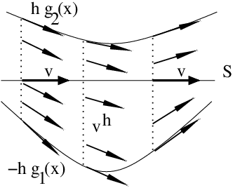
which means that each vhv^{h} is a linear interpolation between the push-forward of the vector field vv from SS onto the external part ∂+Sh\partial^{+}S^{h} of the boundary of ShS^{h} and the other push-forward onto the internal part ∂−Sh\partial^{-}S^{h} of ∂Sh\partial S^{h} (see figure 4.1.1). Indeed, the derivative of the map:
S∋x↦x±h​gi​(x)​n→​(x)S\ni x\mapsto x\pm hg_{i}(x)\vec{n}(x)

is given through:

Id±h​gi​(x)​Π​(x)±h​n→​(x)⊗∇gi​(x).\mbox{Id}\pm hg_{i}(x)\Pi(x)\pm h\vec{n}(x)\otimes\nabla g_{i}(x).

In particular, we see that (4.2) holds.

Refer to caption

Figure 4.1. The vector fields vhv^{h} and vv.

Write now vh=w+(vh−w)v^{h}=w+(v^{h}-w), with:

w⁡(z)=(Id+t​Π​(x))​v​(x),z=x+t​n→​(x).w(z)=\Big(\mbox{Id}+t\Pi(x)\Big)v(x),\qquad z=x+t\vec{n}(x).

We wish to estimate the order of different coefficients in ∇w\nabla w and D⁡(w)D(w). For every τ∈Tx​S\tau\in T_{x}S, x∈Sx\in S, there holds:

(4.4) ∂w∂n→​(z)=Π⁡(x)​v​(x),∂w∂τ​(z)=t∂Π∂((Id+t​Π​(x))−1​τ)(x)v(x)+(Id+tΠ(x))∇v(x)(Id+tΠ(x))−1τ.\begin{split}\frac{\partial w}{\partial\vec{n}}(z)&=\Pi(x)v(x),\\ \frac{\partial w}{\partial\tau}(z)&=t\frac{\partial\Pi}{\partial((\mbox{Id}+t\Pi(x))^{-1}\tau)}(x)v(x)+(\mbox{Id}+t\Pi(x))\nabla v(x)(\mbox{Id}+t\Pi(x))^{-1}\tau.\end{split}

Observe that:

(4.5) (∂w∂τ⋅n→+∂w∂n→⋅τ)(z)=(−∂n→∂τ⋅w+∂w∂n→⋅τ)(z)=−(Π(x)(Id+tΠ(x))−1τ)⋅(Id+tΠ(x))v(x)+Π(x)v(x)⋅τ=0,\begin{split}&\left(\frac{\partial w}{\partial\tau}\cdot\vec{n}+\frac{\partial w}{\partial\vec{n}}\cdot\tau\right)(z)=\left(-\frac{\partial\vec{n}}{\partial\tau}\cdot w+\frac{\partial w}{\partial\vec{n}}\cdot\tau\right)(z)\\ &\qquad\qquad=-\big(\Pi(x)(\mbox{Id}+t\Pi(x))^{-1}\tau\big)\cdot(\mbox{Id}+t\Pi(x))v(x)+\Pi(x)v(x)\cdot\tau\\ &\qquad\qquad=0,\end{split}

because n→⋅w=0\vec{n}\cdot w=0 and the symmetric form Π⁡(x)\Pi(x) commutes with (Id+t​Π​(x))−1(\mbox{Id}+t\Pi(x))^{-1}. Likewise:

(4.6) (∂w∂n→⋅n→)​(z)=0.\left(\frac{\partial w}{\partial\vec{n}}\cdot\vec{n}\right)(z)=0.

To estimate ηT​D​(w)​(z)​τ\eta^{T}D(w)(z)\tau, for τ,η∈Tx​S\tau,\eta\in T_{x}S, notice that:

|ηT(Id+tΠ(x))∇v(x)(Id+tΠ(x))−1τ−ηT(Id+tΠ(x))−1∇v(x)(Id+tΠ(x))−1τ|≤Ct|∇v(x)|,\begin{split}\big|\eta^{T}(\mbox{Id}&+t\Pi(x))\nabla v(x)(\mbox{Id}+t\Pi(x))^{-1}\tau\\ &\qquad-\eta^{T}(\mbox{Id}+t\Pi(x))^{-1}\nabla v(x)(\mbox{Id}+t\Pi(x))^{-1}\tau\big|\leq Ct|\nabla v(x)|,\end{split}

because |(Id+t​Π​(x))−(Id+t​Π​(x))−1|≤C​t|(\mbox{Id}+t\Pi(x))-(\mbox{Id}+t\Pi(x))^{-1}|\leq Ct. Above and in the sequel, CC denotes any positive constant independent of hh. Since τ​(Id+t​Π​(x))−1∈Tx​S\tau(\mbox{Id}+t\Pi(x))^{-1}\in T_{x}S, by (2.3) and (4.4) we obtain:

(4.7) |ηT​D​(w)​(z)​τ|≤C​t​(|v⁡(x)|+|∇v​(x)|).|\eta^{T}D(w)(z)\tau|\leq Ct(|v(x)|+|\nabla v(x)|).

We also have: |∇(vh−w)​(z)|≤C​h|\nabla(v^{h}-w)(z)|\leq Ch and by (4.5), (4.6) and (4.7): |D​(w)​(z)|≤C​h|D(w)(z)|\leq Ch for every z∈Shz\in S^{h}. Hence:

‖D⁡(vh)‖L2​(Sh)2≤C​h3.\|D(v^{h})\|^{2}_{L^{2}(S^{h})}\leq Ch^{3}.

On the other hand, inspecting the terms in (4.4) and recalling that v≠0v\neq 0 (and therefore ∇v≠0\nabla v\neq 0 as well) we see that:

‖∇vh‖L2​(Sh)2≥12​‖∇v‖L2​(Sh)2−C​h3≥C​h.\|\nabla v^{h}\|^{2}_{L^{2}(S^{h})}\geq\frac{1}{2}\|\nabla v\|^{2}_{L^{2}(S^{h})}-Ch^{3}\geq Ch.

The two last inequalities imply that the uniform bound (2.5) is not valid, without the restriction (2.6). Even if SS has no rotational symmetry, the constants ChC_{h} in (2.2) become unbounded as h→0h\to 0.

Remark 4.1.

The construction (4.3) is crucial for the counterexample to work. Indeed, one cannot simply take ’trivial’ extensions v​π∈W1,2​(Sh)v\pi\in W^{1,2}(S^{h}) for the blow-up of ChC_{h}. The reason is that, for any τ∈Tx​S\tau\in T_{x}S, one has:

∂(v​π)∂τ(z)⋅n→=−∂(n→​π)∂τ(z)⋅(vπ)(z)=−Π(x)(Id+tΠ(x))−1τ⋅v(x)=𝒪(1),∂(v​π)∂n→​(z)=0,\begin{split}&\frac{\partial(v\pi)}{\partial\tau}(z)\cdot\vec{n}=-\frac{\partial(\vec{n}\pi)}{\partial\tau}(z)\cdot(v\pi)(z)=-\Pi(x)(\mbox{Id}+t\Pi(x))^{-1}\tau\cdot v(x)=\mathcal{O}(1),\\ &\frac{\partial(v\pi)}{\partial\vec{n}}(z)=0,\end{split}

and thus both ∇(v​π)​(z)\nabla(v\pi)(z) and D​(v​π)​(z)D(v\pi)(z) are of the order 𝒪⁡(1)\mathcal{O}(1). Hence, with a uniform constant CC:

‖∇(v​π)‖L2​(Sh)2≤C​h​‖v‖W1,2​(S)2≤C​h≤C​h​‖v‖L2​(S)2≤C​‖D⁡(v​π)‖L2​(Sh)2.\|\nabla(v\pi)\|_{L^{2}(S^{h})}^{2}\leq Ch\|v\|_{W^{1,2}(S)}^{2}\leq Ch\leq Ch\|v\|_{L^{2}(S)}^{2}\leq C\|D(v\pi)\|_{L^{2}(S^{h})}^{2}.

5. An approximation of ∇u\nabla u

In this section we construct a smooth function RR with skew-symmetric matrix values, approximating ∇u\nabla u on ShS^{h} with the error ‖D⁡(u)‖L2​(Sh)\|D(u)\|_{L^{2}(S^{h})}. The construction relies on Appendix B, where for convenience of the reader we analyse the constant in Korn’s inequality on a fixed, star-shaped with respect to a ball domain (Theorem 10.1). We apply this estimate locally and then use a mollification argument as in [5]. The same approximation result is independently obtained in [10] Theorem 4.3, in the context of the unfolding method in the linearized elasticity.

As always, CC denotes any uniform constant, independent of uu and hh.

Theorem 5.1.

Assume (H1). For every u∈W1,2​(Sh,𝐑n)u\in W^{1,2}(S^{h},\mathbf{R}^{n}) there exists a smooth map R:S⟶s​o​(n)R:S\longrightarrow so(n) such that:

  • (i)

    ‖∇u−R​π‖L2​(Sh)≤C​‖D⁡(u)‖L2​(Sh),\displaystyle\|\nabla u-R\pi\|_{L^{2}(S^{h})}\leq C\|D(u)\|_{L^{2}(S^{h})},

  • (ii)

    ∥∇R∥L2​(S)≤Ch−3/2∥D(u)∥L2​(Sh).\displaystyle\|\nabla R\|_{L^{2}(S)}\leq Ch^{-3/2}\|D(u)\|_{L^{2}(S^{h})}.

Proof.

1. For x∈Sx\in S consider balls in SS and ’cylinders’ in ShS^{h} defined by:

Dx,h=B⁡(x,h)∩S,Bx,h=π−1​(Dx,h)∩Sh.D_{x,h}=B(x,h)\cap S,\qquad B_{x,h}=\pi^{-1}(D_{x,h})\cap S^{h}.

The main observation is that sets Bx,hB_{x,h} are contained in a ball of radius (C2+1)​h(C_{2}+1)h and are star-shaped with respect to a ball of radius r⁡(C1,C2,C3,S)​hr(C_{1},C_{2},C_{3},S)h, when hh is sufficiently small. Hence, an application of Korn’s inequality on Bx,hB_{x,h} (see Theorem 10.1) yields a skew-symmetric matrix Ax,h∈s​o​(n)A_{x,h}\in so(n) such that:

(5.1) ∫Bx,h|∇u​(z)−Ax,h|2​d​z≤C​∫Bx,h|D⁡(u)|2.\int_{B_{x,h}}|\nabla u(z)-A_{x,h}|^{2}~\mbox{d}z\leq C\int_{B_{x,h}}|D(u)|^{2}.

Indeed, recalling the assumption (H1) we see that for hh sufficiently small, Bx,hB_{x,h} are star-shaped with respect to xx and that both the Lipschitz constants of their boundaries and the ratios of their diameters have common bounds.

Our goal is to replace Ax,hA_{x,h} by a matrix R⁡(x)R(x) which depends smoothly on xx. This will allow us to replace Ax,hA_{x,h} by R⁡(π​z)R(\pi z) in (5.1). The desired estimate on ShS^{h} then follows by summing over a suitable family of cylinders. The smoothness of RR will also play essential role in the key estimate in Lemma 6.4.

2. To define R⁡(x)R(x) consider a cut-off function ϑ∈𝒞c∞​([0,1))\vartheta\in\mathcal{C}_{c}^{\infty}([0,1)), with ϑ≥0\vartheta\geq 0, ϑ\vartheta constant in a neighbourhood of 00, and ∫01ϑ=1\int_{0}^{1}\vartheta=1. For each x∈Sx\in S define:

ηx​(z)=ϑ⁡(|π​z−x|/h)∫Shϑ⁡(|π​z−x|/h)​d​z.\displaystyle\eta_{x}(z)=\frac{\vartheta(|\pi z-x|/h)}{\int_{S^{h}}\vartheta(|\pi z-x|/h)~\mbox{d}z}.

Then ηx​(z)=0\eta_{x}(z)=0 for z∉Bx,hz\not\in B_{x,h} and:

∫Shηx​(z)​d​z=1,|ηx|≤Chn,|∇xηx|≤Chn+1\int_{S^{h}}\eta_{x}(z)~\mbox{d}z=1,\qquad|\eta_{x}|\leq\frac{C}{h^{n}},\qquad|\nabla_{x}\eta_{x}|\leq\frac{C}{h^{n+1}}

Define R⁡(x)R(x) as the average:

R⁡(x)=∫Shηx​(z)​ skew​(∇u​(z))​d​z,R(x)=\int_{S^{h}}\eta_{x}(z)\mbox{ skew}(\nabla u(z))~\mbox{d}z,

where skew​(F)=(F−FT)/2\mbox{skew}(F)=(F-F^{T})/2 denotes the skew-symmetric part of a given matrix FF. Since ∫ηx=1\int\eta_{x}=1, we have:

R⁡(x)−Ax,h=∫Shηx​(z)​ skew​(∇u​(z)−Ax,h)​d​z,R(x)-A_{x,h}=\int_{S^{h}}\eta_{x}(z)\mbox{ skew}(\nabla u(z)-A_{x,h})~\mbox{d}z,

and by the Cauchy-Schwarz inequality, noting that |skew​(F)|≤C​|F||\mbox{skew}(F)|\leq C|F| we obtain:

(5.2) |R⁡(x)−Ax,h|2≤C​(∫Shηx​(z)​|∇u​(z)−Ax,h|​d​z)2≤Chn​∫Bx,h|D⁡(u)|2.|R(x)-A_{x,h}|^{2}\leq C\left(\int_{S^{h}}\eta_{x}(z)|\nabla u(z)-A_{x,h}|~\mbox{d}z\right)^{2}\leq\frac{C}{h^{n}}\int_{B_{x,h}}|D(u)|^{2}.

To estimate the derivative of RR we use that:

∫Sh∇xηx​(z)​d​z=∇x(∫Shηx​(z)​d​z)=0.\int_{S^{h}}\nabla_{x}\eta_{x}(z)~\mbox{d}z=\nabla_{x}\left(\int_{S^{h}}\eta_{x}(z)~\mbox{d}z\right)=0.

Thus:

∇R​(x)=∫Sh(∇xηx)​ skew​(∇u)=∫Sh(∇xηx)​ skew​(∇u−Ax,h)\nabla R(x)=\int_{S^{h}}\left(\nabla_{x}\eta_{x}\right)\mbox{ skew}(\nabla u)=\int_{S^{h}}\left(\nabla_{x}\eta_{x}\right)\mbox{ skew}(\nabla u-A_{x,h})

and by (5.1):

(5.3) |∇R​(x)|2≤∫Bx,h|∇xηx|2⋅∫Bx,h|∇u−Ax,h|2≤Chn+2​∫Bx,h|D⁡(u)|2.|\nabla R(x)|^{2}\leq\int_{B_{x,h}}\left|\nabla_{x}\eta_{x}\right|^{2}\cdot\int_{B_{x,h}}\left|\nabla u-A_{x,h}\right|^{2}\leq\frac{C}{h^{n+2}}\int_{B_{x,h}}|D(u)|^{2}.

Similarly, we get for all x′∈Dx,hx^{\prime}\in D_{x,h}:

(5.4) |∇R​(x′)|2≤Chn+2​∫Bx′,h|D⁡(u)|2≤Chn+2​∫2​Bx,h|D⁡(u)|2,|\nabla R(x^{\prime})|^{2}\leq\frac{C}{h^{n+2}}\int_{B_{x^{\prime},h}}|D(u)|^{2}\leq\frac{C}{h^{n+2}}\int_{2B_{x,h}}|D(u)|^{2},

where 2​Bx,h=π−1​(Dx,2​h)∩Sh2B_{x,h}=\pi^{-1}(D_{x,2h})\cap S^{h}. From this, by the fundamental theorem of calculus:

|R⁡(x′′)−R⁡(x)|2≤Chn​∫2​Bx,h|D⁡(u)|2∀x′′∈Dx,h.|R(x^{\prime\prime})-R(x)|^{2}\leq\frac{C}{h^{n}}\int_{2B_{x,h}}|D(u)|^{2}\qquad\forall x^{\prime\prime}\in D_{x,h}.

In combination with (5.1) and (5.2) this yields:

(5.5) ∫Bx,h|∇u​(z)−R⁡(π​z)|2​d​z≤C​∫2​Bx,h|D⁡(u)|2.\int_{B_{x,h}}|\nabla u(z)-R(\pi z)|^{2}~\mbox{d}z\leq C\int_{2B_{x,h}}|D(u)|^{2}.

Now cover ShS^{h} with a family {Bxi,h}i=1N⁡(h)\{B_{x_{i},h}\}_{i=1}^{N(h)} so that the covering number of {2​Bxi,h}i=1N⁡(h)\{2B_{x_{i},h}\}_{i=1}^{N(h)} is independent of hh. A possible argument for the existence of such a covering goes as follows. The surface SS is contained in the finite union of balls ∪i=1N⁡(h)B(xi,h/2)\cup_{i=1}^{N(h)}B(x_{i},h/2) where ki∈(h2​ℤ)nk_{i}\in(\frac{h}{2}\mathbb{Z})^{n}. Fix a one-to-one map ki↦xi∈S∩B⁡(ki,h/2)k_{i}\mapsto x_{i}\in S\cap B(k_{i},h/2), so that Sh=∪iBxi,hS^{h}=\cup_{i}B_{x_{i},h}. Then, if z∈2​Bxi,hz\in 2B_{x_{i},h} there must be π⁡(z)∈B⁡(xi,2​h)\pi(z)\in B(x_{i},2h), so that |ki−π⁡(z)|≤|ki−xi|+|π⁡(z)−xi|≤5​h/2|k_{i}-\pi(z)|\leq|k_{i}-x_{i}|+|\pi(z)-x_{i}|\leq 5h/2. Therefore ki∈B⁡(x,5​h/2)∩(h2​ℤ)nk_{i}\in B(x,5h/2)\cap(\frac{h}{2}\mathbb{Z})^{n}. The cardinality of this last set is bounded by 10n10^{n}, which must as well be a covering number for the family {2​Bxi,h}i=1N⁡(h)\{2B_{x_{i},h}\}_{i=1}^{N(h)}.

Summing (5.5) over i=1​…​Ni=1\ldots N proves (i). Finally, integrating (5.4) on Dx,hD_{x,h} we get;

∫Dx,h|∇R​(x′)|2​d​x′≤Ch3​∫2​Bx,h|D⁡(u)|2,\int_{D_{x,h}}|\nabla R(x^{\prime})|^{2}~\mbox{d}x^{\prime}\leq\frac{C}{h^{3}}\int_{2B_{x,h}}|D(u)|^{2},

and using the same covering as before we obtain (ii).  

Following the same argument, we will prove a uniform Poincaré inequality in thin domains - see Theorem 12.1 in Appendix D.

6. The key estimates

Let u¯:S⟶𝐑n\bar{u}:S\longrightarrow\mathbf{R}^{n} be the average of uu in the normal direction:

(6.1) u¯​(x)=⨏−g1h​(x)g2h​(x)u⁡(x+t​n→​(x))​d​t∀x∈S.\bar{u}(x)=\fint_{-g_{1}^{h}(x)}^{g_{2}^{h}(x)}u(x+t\vec{n}(x))~\mbox{d}t\qquad\forall x\in S.

In this section we will establish four useful estimates on various components of u¯\bar{u} and their derivatives.

The first estimate on ∇u¯\nabla\bar{u}, is an extension of the previous Theorem 5.1:

Lemma 6.1.

Assume (H1). For every u∈W1,2​(Sh,𝐑n)u\in W^{1,2}(S^{h},\mathbf{R}^{n}) there holds:

∥∇u¯−Rt​a​n∥L2​(S)≤Ch1/2∥u∥W1,2​(Sh)+Ch−1/2∥D(u)∥L2​(Sh),\|\nabla\bar{u}-R_{tan}\|_{L^{2}(S)}\leq Ch^{1/2}\|u\|_{W^{1,2}(S^{h})}+Ch^{-1/2}\|D(u)\|_{L^{2}(S^{h})},

where the subscript ’t​a​ntan’ refers to the tangential components of the appropriate matrix valued function, that is: Rt​a​n​(x)​n→​(x)=0R_{tan}(x)\vec{n}(x)=0 and Rt​a​n​(x)​τ=R⁡(x)​τR_{tan}(x)\tau=R(x)\tau for all x∈Sx\in S and τ∈Tx​S\tau\in T_{x}S.

Proof.

Through a direct calculation one checks that for every x∈Sx\in S and τ∈Tx​S\tau\in T_{x}S there holds:

|∂τu¯​(x)−⨏−g1h​(x)g2h​(x)∇u​(x+t​n→​(x))⋅{τ+t​∂τn→​(x)}​d​t|≤Ch​(|∂τg1h​(x)|+|∂τg2h​(x)|)⋅∫−g1h​(x)g2h​(x)|∂n→u⁡(x+t​n→​(x))|​d​t≤C​∫−g1h​(x)g2h​(x)|∇u|​d​t\begin{split}&\left|\partial_{\tau}\bar{u}(x)-\fint_{-g_{1}^{h}(x)}^{g_{2}^{h}(x)}\nabla u(x+t\vec{n}(x))\cdot\left\{\tau+t\partial_{\tau}\vec{n}(x)\right\}~\mbox{d}t\right|\\ &\qquad\leq\frac{C}{h}\left(|\partial_{\tau}g_{1}^{h}(x)|+|\partial_{\tau}g_{2}^{h}(x)|\right)\cdot\int_{-g_{1}^{h}(x)}^{g_{2}^{h}(x)}|\partial_{\vec{n}}u(x+t\vec{n}(x))|~\mbox{d}t\leq C\int_{-g_{1}^{h}(x)}^{g_{2}^{h}(x)}|\nabla u|~\mbox{d}t\end{split}

and:

⨏−g1h​(x)g2h​(x)|∇u​(x+t​n→​(x))⋅(τ+t​∂τn→​(x))−R⁡(x)​τ|​d​t≤C​∫−g1h​(x)g2h​(x)|∇u|​d​t+⨏−g1h​(x)g2h​(x)|∇u​(x+t​n→​(x))−R⁡(x)|​d​t.\begin{split}&\fint_{-g_{1}^{h}(x)}^{g_{2}^{h}(x)}\left|\nabla u(x+t\vec{n}(x))\cdot\left(\tau+t\partial_{\tau}\vec{n}(x)\right)-R(x)\tau\right|~\mbox{d}t\\ &\qquad\qquad\leq C\int_{-g_{1}^{h}(x)}^{g_{2}^{h}(x)}|\nabla u|~\mbox{d}t+\fint_{-g_{1}^{h}(x)}^{g_{2}^{h}(x)}|\nabla u(x+t\vec{n}(x))-R(x)|~\mbox{d}t.\end{split}

Hence, by Theorem 5.1 (i):

‖∇u¯−Rt​a​n‖L2​(S)2≤C​∫S{h​∫−g1h​(x)g2h​(x)|∇u|2​d​t+h−1​⨏−g1h​(x)g2h​(x)|∇u−R​π|2​d​t}​d​x≤C​h​‖∇u‖L2​(Sh)2+C​h−1​‖D⁡(u)‖L2​(Sh)2.\begin{split}\|\nabla\bar{u}-R_{tan}\|_{L^{2}(S)}^{2}&\leq C\int_{S}\left\{h\int_{-g_{1}^{h}(x)}^{g_{2}^{h}(x)}|\nabla u|^{2}~\mbox{d}t+h^{-1}\fint_{-g_{1}^{h}(x)}^{g_{2}^{h}(x)}|\nabla u-R\pi|^{2}~\mbox{d}t\right\}~\mbox{d}x\\ &\leq Ch\|\nabla u\|_{L^{2}(S^{h})}^{2}+Ch^{-1}\|D(u)\|_{L^{2}(S^{h})}^{2}.\end{split}


In order to estimate the normal part u¯\bar{u}, we will use the following bounds:

Lemma 6.2.

Recall that ∂Sh=∂−Sh∪∂+Sh\partial S^{h}=\partial^{-}S^{h}\cup\partial^{+}S^{h}, with:

(6.2) ∂−Sh={x−g1h​(x)​n→​(x);x∈S},∂+Sh={x+g2h​(x)​n→​(x);x∈S}.\begin{split}\partial^{-}S^{h}&=\{x-g_{1}^{h}(x)\vec{n}(x);~x\in S\},\\ \partial^{+}S^{h}&=\{x+g_{2}^{h}(x)\vec{n}(x);~x\in S\}.\end{split}
  • (i)

    If (H1) holds then |n→h​(z)−n→​(π⁡(z))|≤C​h|\vec{n}^{h}(z)-\vec{n}(\pi(z))|\leq Ch for all z∈∂+Shz\in\partial^{+}S^{h} and |n→h​(z)+n→​(π⁡(z))|≤C​h|\vec{n}^{h}(z)+\vec{n}(\pi(z))|\leq Ch for all z∈∂−Shz\in\partial^{-}S^{h}.

  • (ii)

    If (H2) holds then:

    |n→h​(z)+n→​(π⁡(z))+∇g1h​(π⁡(z))|≤Ch2∀z∈∂−Sh,|n→h​(z)−n→​(π⁡(z))+∇g2h​(π⁡(z))|≤Ch2∀z∈∂+Sh.\begin{split}|\vec{n}^{h}(z)+\vec{n}(\pi(z))+\nabla g_{1}^{h}(\pi(z))|&\leq Ch^{2}\qquad\forall z\in\partial^{-}S^{h},\\ |\vec{n}^{h}(z)-\vec{n}(\pi(z))+\nabla g_{2}^{h}(\pi(z))|&\leq Ch^{2}\qquad\forall z\in\partial^{+}S^{h}.\end{split}

Let now u∈W1,2​(Sh,𝐑n)u\in W^{1,2}(S^{h},\mathbf{R}^{n}).

  • (iii)

    |∂n→(u⋅n→)​(z)|≤|D⁡(u)​(z)|{\displaystyle|\partial_{\vec{n}}(u\cdot\vec{n})(z)|\leq|D(u)(z)|} for all z∈Shz\in S^{h}.

  • (iv)

    If (H1) holds and u⋅n→h=0u\cdot\vec{n}^{h}=0 on ∂+Sh\partial^{+}S^{h}, then:

    ‖u⋅n→‖L2​(∂+Sh)≤C​h1/2​‖u‖W1,2​(Sh).\displaystyle\|u\cdot\vec{n}\|_{L^{2}(\partial^{+}S^{h})}\leq Ch^{1/2}\|u\|_{W^{1,2}(S^{h})}.
  • (v)

    If (H2) holds and u⋅n→h=0u\cdot\vec{n}^{h}=0 on ∂Sh\partial S^{h}:

    ∫S|u⁡(x−g1h​(x)CLOSEn→(x))⋅∇g1h(x)+u(x+g2h(x)n→(x))⋅∇g2h(x)|2dx≤C​h​∫Sh|D⁡(u)|2+C​h3​‖u‖W1,2​(Sh)2.\begin{split}\int_{S}|u(x-g_{1}^{h}(x)&\vec{n}(x))\cdot\nabla g_{1}^{h}(x)+u(x+g_{2}^{h}(x)\vec{n}(x))\cdot\nabla g_{2}^{h}(x)|^{2}~\mathrm{d}x\\ &\leq Ch\int_{S^{h}}|D(u)|^{2}+Ch^{3}\|u\|_{W^{1,2}(S^{h})}^{2}.\end{split}
Proof.

(i) is obvious. To prove (ii) observe, for example, that on ∂+Sh\partial^{+}S^{h} the normal n→h​(z)\vec{n}^{h}(z) is parallel to n→​(π⁡(z))−∇g2h​(π⁡(z))+w\vec{n}(\pi(z))-\nabla g_{2}^{h}(\pi(z))+w, where |w|≤C|g2h(π(x))∇g2h(π(z))|≤Ch2|w|\leq C|g_{2}^{h}(\pi(x))\nabla g_{2}^{h}(\pi(z))|\leq Ch^{2}. Normalising this vector we conclude the second inequality in (ii). The first one follows in the same manner.

(iii) follows from: ∂n→(u⋅n→)=D⁡(u)​n→⋅n→\partial_{\vec{n}}(u\cdot\vec{n})=D(u)\vec{n}\cdot\vec{n}.

To prove (iv), use (i) and the trace theorem in Appendix D:

‖u⋅n→‖L2​(∂+Sh)=‖u⋅(n→−n→h)‖L2​(∂+Sh)≤C​h1/2​‖u‖W1,2​(Sh).\|u\cdot\vec{n}\|_{L^{2}(\partial^{+}S^{h})}=\|u\cdot(\vec{n}-\vec{n}^{h})\|_{L^{2}(\partial^{+}S^{h})}\leq Ch^{1/2}\|u\|_{W^{1,2}(S^{h})}.

For (v), use (ii), (iii) and Theorem 12.3:

∫S|u⁡(x+g2h​(x)​n→​(x))⋅∇g2h​(x)+u⁡(x−g1h​(x)​n→​(x))⋅∇g1h​(x)|2​𝑑x≤∫S|u⁡(x+g2h​(x)​n→​(x))⋅n→​(x)−u⁡(x−g1h​(x)​n→​(x))⋅n→​(x)|2​dx+C​h4​∫∂Sh|u|2=∫S|∫−g1h​(x)g2h​(x)∂n→(u⋅n→)​(x+t​n→​(x))​dt|2​dx+C​h4​∫∂Sh|u|2≤C​h​∫Sh|D⁡(u)|2+C​h3​‖u‖W1,2​(Sh)2.\begin{split}&\int_{S}|u(x+g_{2}^{h}(x)\vec{n}(x))\cdot\nabla g_{2}^{h}(x)+u(x-g_{1}^{h}(x)\vec{n}(x))\cdot\nabla g_{1}^{h}(x)|^{2}~\mathrm{d}x\\ &\leq\int_{S}|u(x+g_{2}^{h}(x)\vec{n}(x))\cdot\vec{n}(x)-u(x-g_{1}^{h}(x)\vec{n}(x))\cdot\vec{n}(x)|^{2}~\mathrm{d}x+Ch^{4}\int_{\partial S^{h}}|u|^{2}\\ &\qquad\qquad=\int_{S}\left|\int_{-g_{1}^{h}(x)}^{g_{2}^{h}(x)}\partial_{\vec{n}}(u\cdot\vec{n})(x+t\vec{n}(x))~\mathrm{d}t\right|^{2}~\mathrm{d}x+Ch^{4}\int_{\partial S^{h}}|u|^{2}\\ &\qquad\qquad\leq Ch\int_{S^{h}}|D(u)|^{2}+Ch^{3}\|u\|_{W^{1,2}(S^{h})}^{2}.\end{split}


Lemma 6.3.

Assume (H1) and let u∈W1,2​(Sh,𝐑n)u\in W^{1,2}(S^{h},\mathbf{R}^{n}) satisfy u⋅n→h=0u\cdot\vec{n}^{h}=0 on ∂+Sh\partial^{+}S^{h}. Then:

‖u¯⋅n→‖L2​(S)≤C​h1/2​‖u‖W1,2​(Sh).\|\bar{u}\cdot\vec{n}\|_{L^{2}(S)}\leq Ch^{1/2}\|u\|_{W^{1,2}(S^{h})}.
Proof.

By Lemma 6.2 (iv) and (i), for every z=x+t​n→​(x)∈Shz=x+t\vec{n}(x)\in S^{h} we obtain:

|u(x+tn→(x))⋅n→(x)|2≤(|u(x+g2h(x)n→(x))⋅n→(x)|+∫−g1h​(x)g2h​(x)|D(u)|)2≤C⋅|u⁡(x+g2h​(x)​n→​(x))⋅(n→​(x)−n→h​(x+g2h​(x)​n→​(x)))|2+C​h​∫−g1h​(x)g2h​(x)|D⁡(u)|2≤C​h2​|u⁡(x+g2h​(x)​n→​(x))|2+C​h​∫−g1h​(x)g2h​(x)|D⁡(u)|2.\begin{split}|u(x+&t\vec{n}(x))\cdot\vec{n}(x)|^{2}\leq\left(|u(x+g_{2}^{h}(x)\vec{n}(x))\cdot\vec{n}(x)|+\int_{-g_{1}^{h}(x)}^{g_{2}^{h}(x)}|D(u)|\right)^{2}\\ &\leq C\cdot\left|u(x+g_{2}^{h}(x)\vec{n}(x))\cdot\left(\vec{n}(x)-\vec{n}^{h}(x+g_{2}^{h}(x)\vec{n}(x))\right)\right|^{2}+Ch\int_{-g_{1}^{h}(x)}^{g_{2}^{h}(x)}|D(u)|^{2}\\ &\leq Ch^{2}|u(x+g_{2}^{h}(x)\vec{n}(x))|^{2}+Ch\int_{-g_{1}^{h}(x)}^{g_{2}^{h}(x)}|D(u)|^{2}.\end{split}

Hence by Theorem 12.3:

(6.3) ‖u¯⋅n→‖L2​(S)2≤Ch​∫S∫−g1h​(x)g2h​(x)|u⁡(x+t​n→​(x))⋅n→​(x)|2​d​t​d​x≤Ch​(h3​‖u‖L2​(∂Sh)2+h2​‖D⁡(u)‖L2​(Sh)2)≤C​h​‖∇u‖L2​(Sh)2.\begin{split}\|\bar{u}\cdot\vec{n}\|_{L^{2}(S)}^{2}&\leq\frac{C}{h}\int_{S}\int_{-g_{1}^{h}(x)}^{g_{2}^{h}(x)}|u(x+t\vec{n}(x))\cdot\vec{n}(x)|^{2}~\mbox{d}t~\mbox{d}x\\ &\leq\frac{C}{h}\left(h^{3}\|u\|_{L^{2}(\partial S^{h})}^{2}+h^{2}\|D(u)\|_{L^{2}(S^{h})}^{2}\right)\leq Ch\|\nabla u\|_{L^{2}(S^{h})}^{2}.\end{split}


The next, key estimate, is on the gradient of u¯⋅n→\bar{u}\cdot\vec{n}. It is obtained using the divergence theorem on the surface SS:

Lemma 6.4.

Assume (H1) and let u∈W1,2​(Sh,𝐑n)u\in W^{1,2}(S^{h},\mathbf{R}^{n}) satisfy u⋅n→h=0u\cdot\vec{n}^{h}=0 on ∂+Sh\partial^{+}S^{h}. Then:

‖∇(u¯⋅n→)‖L2​(S)+‖R​n→‖L2​(S)≤C(∥u¯∥L2​(S)+∥u∥W1,2​(Sh)+h−1/2∥D(u)∥L2​(Sh))+C​(h−1​‖u‖W1,2​(Sh)⋅‖D⁡(u)‖L2​(Sh))1/2.\begin{split}\|\nabla(\bar{u}\cdot\vec{n})\|_{L^{2}(S)}+\|R\vec{n}\|_{L^{2}(S)}&\leq C\left(\|\bar{u}\|_{L^{2}(S)}+\|u\|_{W^{1,2}(S^{h})}+h^{-1/2}\|D(u)\|_{L^{2}(S^{h})}\right)\\ &\quad+C\left(h^{-1}\|u\|_{W^{1,2}(S^{h})}\cdot\|D(u)\|_{L^{2}(S^{h})}\right)^{1/2}.\end{split}
Proof.

First note that ‖R​n→‖L2​(S)=‖n→T​Rt​a​n‖L2​(S)\|R\vec{n}\|_{L^{2}(S)}=\|\vec{n}^{T}R_{tan}\|_{L^{2}(S)}, since n→​R​n→=0\vec{n}R\vec{n}=0 and R∈s​o​(n)R\in so(n). To prove the desired estimate we use the Hilbert space identity:

‖a‖2+‖b‖2=‖a−b‖2+2​⟨a,b⟩\|a\|^{2}+\|b\|^{2}=\|a-b\|^{2}+2\langle a,b\rangle

with a=∇(u¯⋅n→)a=\nabla(\bar{u}\cdot\vec{n}) and b=n→T​Rt​a​nb=\vec{n}^{T}R_{tan}.

Integration by parts shows that:

(6.4) ⟨a,b⟩=|∫S(n→​Rt​a​n)⋅∇(u¯⋅n→)|≤C​‖u¯⋅n→‖L2​(S)​(‖R‖L2​(S)+‖∇(n→​Rt​a​n)‖L2​(S))≤C​‖u¯⋅n→‖L2​(S)​‖R‖W1,2​(S)≤C∥u¯⋅n→∥L2​(S)(h−3/2∥D(u)∥L2​(Sh)+h−1/2∥∇u∥L2​(Sh))≤C​h−1​‖u‖W1,2​(Sh)⋅‖D⁡(u)‖L2​(Sh)+C​‖u‖W1,2​(Sh)2,\begin{split}\langle a,b\rangle&=\left|\int_{S}(\vec{n}R_{tan})\cdot\nabla(\bar{u}\cdot\vec{n})\right|\leq C\|\bar{u}\cdot\vec{n}\|_{L^{2}(S)}\left(\|R\|_{L^{2}(S)}+\|\nabla(\vec{n}R_{tan})\|_{L^{2}(S)}\right)\\ &\leq C\|\bar{u}\cdot\vec{n}\|_{L^{2}(S)}\|R\|_{W^{1,2}(S)}\\ &\leq C\|\bar{u}\cdot\vec{n}\|_{L^{2}(S)}\left(h^{-3/2}\|D(u)\|_{L^{2}(S^{h})}+h^{-1/2}\|\nabla u\|_{L^{2}(S^{h})}\right)\\ &\leq Ch^{-1}\|u\|_{W^{1,2}(S^{h})}\cdot\|D(u)\|_{L^{2}(S^{h})}+C\|u\|_{W^{1,2}(S^{h})}^{2},\end{split}

where we applied the divergence theorem, Theorem 5.1 and Lemma 6.3.

On the other hand a=n→T∇u¯+u¯⋅∇n→a=\vec{n}^{T}\nabla\bar{u}+\bar{u}\cdot\nabla\vec{n}, so by Lemma 6.1:

(6.5) ‖a−b‖≤C⁡(‖u¯‖L2​(S)+‖∇u¯−Rt​a​n‖L2​(S))≤C∥u¯∥L2​(S)+Ch1/2∥u∥W1,2​(Sh)+Ch−1/2∥D(u)∥L2​(Sh).\begin{split}\|a-b\|&\leq C\left(\|\bar{u}\|_{L^{2}(S)}+\|\nabla\bar{u}-R_{tan}\|_{L^{2}(S)}\right)\\ &\leq C\|\bar{u}\|_{L^{2}(S)}+Ch^{1/2}\|u\|_{W^{1,2}(S^{h})}+Ch^{-1/2}\|D(u)\|_{L^{2}(S^{h})}.\end{split}

Combining (6.4) and (6.5) proves the result.  

Finally, in presence of the stronger condition (H2), we have an additional bound:

Lemma 6.5.

Assume (H2) and let u∈W1,2​(Sh,𝐑n)u\in W^{1,2}(S^{h},\mathbf{R}^{n}), u⋅n→h=0u\cdot\vec{n}^{h}=0 on ∂Sh\partial S^{h}. Then:

1h∫S|u¯⋅∇(g1h+g2h)|≤Ch1/2∥u∥W1,2​(Sh)+Ch−1/2∥D(u)∥L2​(Sh).\frac{1}{h}\int_{S}|\bar{u}\cdot\nabla(g_{1}^{h}+g_{2}^{h})|\leq Ch^{1/2}\|u\|_{W^{1,2}(S^{h})}+Ch^{-1/2}\|D(u)\|_{L^{2}(S^{h})}.
Proof.

We have:

1h∫S|u¯⋅∇(g1h+g2h)|≤1h​∫S|u⁡(x−g1h​(x)​n→​(x))⋅∇g1h​(x)+u⁡(x+g2h​(x)​n→​(x))⋅∇g2h​(x)|​d​x+C​‖u−u¯​π‖L1​(∂Sh)≤Ch−1/2∥D(u)∥L2​(S)+Ch1/2∥u∥W1,2​(Sh)+Ch1/2∥∇u∥L2​(Sh).\begin{split}\frac{1}{h}\int_{S}|\bar{u}&\cdot\nabla(g_{1}^{h}+g_{2}^{h})|\\ &\leq\frac{1}{h}\int_{S}|u(x-g_{1}^{h}(x)\vec{n}(x))\cdot\nabla g_{1}^{h}(x)+u(x+g_{2}^{h}(x)\vec{n}(x))\cdot\nabla g_{2}^{h}(x)|~\mbox{d}x\\ &\quad+C\|u-\bar{u}\pi\|_{L^{1}(\partial S^{h})}\\ &\leq Ch^{-1/2}\|D(u)\|_{L^{2}(S)}+Ch^{1/2}\|u\|_{W^{1,2}(S^{h})}+Ch^{1/2}\|\nabla u\|_{L^{2}(S^{h})}.\end{split}

The last inequality follows from Lemma 6.2 (v) and from an easy bound: ‖u−u¯​π‖L1​(∂Sh)≤C​h1/2​‖∇u‖L2​(Sh)\|u-\bar{u}\pi\|_{L^{1}(\partial S^{h})}\leq Ch^{1/2}\|\nabla u\|_{L^{2}(S^{h})}.  

7. A proof of main theorems

In this section we will prove the uniform Korn’s estimate:

(7.1) ‖u‖W1,2​(Sh)≤C​‖D⁡(u)‖L2​(Sh),\|u\|_{W^{1,2}(S^{h})}\leq C\|D(u)\|_{L^{2}(S^{h})},

under the angle constraints (2.4) or (2.6). We argue by contradiction; assume thus that (7.1) is not valid, for any uniform constant CC. Hence, there exist sequences hn⟶0h_{n}\longrightarrow 0 and uhn∈W1,2​(Shn)u^{h_{n}}\in W^{1,2}(S^{h_{n}}) (for simplicity we will write hh instead of hnh_{n}) such that the assumptions of Theorem 2.1 or 2.2 are satisfied, but:

(7.2) h−1/2∥uh∥W1,2​(Sh)=1 and h−1/2∥D(uh)∥L2​(Sh)⟶0 as h⟶0.h^{-1/2}\|u^{h}\|_{W^{1,2}(S^{h})}=1\quad\mbox{ and }\quad h^{-1/2}\|D(u^{h})\|_{L^{2}(S^{h})}\longrightarrow 0\qquad\mbox{ as }h\longrightarrow 0.

For the proof of Theorem 2.1 we will assume that uh⋅n→h=0u^{h}\cdot\vec{n}^{h}=0 on ∂+Sh\partial^{+}S^{h}. The case of the tangency condition on ∂−Sh\partial^{-}S^{h} is proved exactly the same.

Notice that (7.2) immediately gives, through Lemmas 6.3, 6.1 and 6.4, that:

(7.3) limh→0(‖u¯h⋅n→‖L2​(S)+‖∇u¯h−Rt​a​nh‖L2​(S))=0,\displaystyle\displaystyle\lim_{h\to 0}\left(\|\bar{u}^{h}\cdot\vec{n}\|_{L^{2}(S)}+\|\nabla\bar{u}^{h}-R_{tan}^{h}\|_{L^{2}(S)}\right)=0,
(7.4) limh→0(‖∇(u¯h⋅n→)‖L2​(S)+‖Rh​n→‖L2​(S))≤C​lim suph→0‖u¯h‖L2​(S).\displaystyle\displaystyle\lim_{h\to 0}\left(\|\nabla(\bar{u}^{h}\cdot\vec{n})\|_{L^{2}(S)}+\|R^{h}\vec{n}\|_{L^{2}(S)}\right)\leq C\limsup_{h\to 0}\|\bar{u}^{h}\|_{L^{2}(S)}.

Also, Lemma 6.5 implies that under the assumption (H2):

(7.5) limh→0∫S|u¯h⋅∇(g1+g2)|=0,\lim_{h\to 0}\int_{S}|\bar{u}^{h}\cdot\nabla(g_{1}+g_{2})|=0,

where we used that the sequence u¯h\bar{u}^{h} is bounded in L1​(S)L^{1}(S), again in view of (7.2).

A contradiction will be derived in several steps. In particular, the tangential component of the average u¯\bar{u}:

u¯t​a​nh​(x)=u¯h​(x)−(u¯h⋅n→)⋅n→​(x)∈Tx​S.\bar{u}^{h}_{tan}(x)=\bar{u}^{h}(x)-(\bar{u}^{h}\cdot\vec{n})\cdot\vec{n}(x)\in T_{x}S.

will be estimated using the Korn inequality on hypersurfaces (see Appendix C). The conditions (2.4) and (2.6) assumed in Theorems 2.1 and 2.2 will be used in full (not just for rotations as in Theorem 2.3).

Proof of Theorems 2.1 and 2.2.

1. Applying Theorem 11.2 to each tangent vector field u¯t​a​nh\bar{u}^{h}_{tan}, we obtain a sequence v0h∈ℐ⁡(S)v_{0}^{h}\in\mathcal{I}(S) such that:

‖u¯t​a​nh−v0h‖W1,2​(S)≤C​‖D⁡(u¯t​a​nh)‖L2​(S).\|\bar{u}^{h}_{tan}-v_{0}^{h}\|_{W^{1,2}(S)}\leq C\|D(\bar{u}^{h}_{tan})\|_{L^{2}(S)}.

For every x∈Sx\in S and τ∈Tx​S\tau\in T_{x}S there holds:

|∂τu¯t​a​nh​(x)⋅τ|=|∂τu¯h​(x)⋅τ−(u¯h⋅n→)​(x)⋅∂τn→​(x)|≤|∂τu¯h​(x)−Rh​(x)​τ|+C​|(u¯h⋅n→)​(x)|,\begin{split}|\partial_{\tau}\bar{u}^{h}_{tan}(x)\cdot\tau|&=|\partial_{\tau}\bar{u}^{h}(x)\cdot\tau-(\bar{u}^{h}\cdot\vec{n})(x)\cdot\partial_{\tau}\vec{n}(x)|\\ &\leq|\partial_{\tau}\bar{u}^{h}(x)-R^{h}(x)\tau|+C|(\bar{u}^{h}\cdot\vec{n})(x)|,\end{split}

as Rh​(x)∈s​o​(n)R^{h}(x)\in so(n). Thus, by (7.3):

‖D⁡(u¯t​a​nh)‖L2​(S)≤C⁡(‖∇u¯h−Rt​a​nh‖L2​(S)+‖u¯h⋅n→‖L2​(S))⟶0 as ​h⟶0.\|D(\bar{u}^{h}_{tan})\|_{L^{2}(S)}\leq C\left(\|\nabla\bar{u}^{h}-R^{h}_{tan}\|_{L^{2}(S)}+\|\bar{u}^{h}\cdot\vec{n}\|_{L^{2}(S)}\right)\longrightarrow 0\qquad\mbox{ as }h\longrightarrow 0.

Therefore:

(7.6) limh→0‖u¯t​a​nh−v0h‖W1,2​(S)=0.\lim_{h\to 0}\|\bar{u}^{h}_{tan}-v_{0}^{h}\|_{W^{1,2}(S)}=0.

2. Let ℙ\mathbb{P} be the orthogonal projection (with respect to the L2​(S)L^{2}(S) norm) of the space ℐ⁡(S)\mathcal{I}(S) onto its subspace VV, which we take to be the whole ℐ⁡(S)\mathcal{I}(S) in case of Theorem 2.1 and ℐg1,g2​(S)\mathcal{I}_{g_{1},g_{2}}(S) in case of Theorem 2.2. Call v1h=ℙ​v0h∈Vv_{1}^{h}=\mathbb{P}v_{0}^{h}\in V and v2h=v0h−v1h∈V⟂v_{2}^{h}=v_{0}^{h}-v_{1}^{h}\in V^{\perp}. In both cases (3.1) implies:

(7.7) ‖uh‖L2​(Sh)≤C​‖uh−v1h​π‖L2​(Sh).\|u^{h}\|_{L^{2}(S^{h})}\leq C\|u^{h}-v_{1}^{h}\pi\|_{L^{2}(S^{h})}.

We now prove that:

(7.8) limh→0‖v2h‖L2​(S)=0.\lim_{h\to 0}\|v_{2}^{h}\|_{L^{2}(S)}=0.

In case of Theorem 2.1, when V⟂={0}V^{\perp}=\{0\}, (7.8) is trivial, so we concentrate on the case of Theorem 2.2. Notice that then, (7.5) and (7.6) yield:

(7.9) ∫S|v2h⋅∇(g1+g2)|=∫S|v0h⋅∇(g1+g2)|≤C∥u¯ht​a​n−v0h∥L1​(S)+C∫S|u¯h⋅∇(g1+g2)|⟶0 as h⟶0.\begin{split}&\int_{S}|v_{2}^{h}\cdot\nabla(g_{1}+g_{2})|=\int_{S}|v_{0}^{h}\cdot\nabla(g_{1}+g_{2})|\\ &\qquad\leq C\|\bar{u}^{h}_{tan}-v_{0}^{h}\|_{L^{1}(S)}+C\int_{S}|\bar{u}^{h}\cdot\nabla(g_{1}+g_{2})|\longrightarrow 0\qquad\mbox{ as }h\longrightarrow 0.\end{split}

Since all norms in the finitely dimensional space V⟂V^{\perp} are equivalent, we have:

(7.10) ‖v2h‖L2​(S)≤C​∫S|v2h⋅∇(g1+g2)|.\|v_{2}^{h}\|_{L^{2}(S)}\leq C\int_{S}|v_{2}^{h}\cdot\nabla(g_{1}+g_{2})|.

Indeed, the right hand side of (7.10) provides a norm on the space in question. Now, (7.9) and (7.10) clearly imply (7.8).

3. Using the Poincaré inequality on each segment [−g1h​(x),g2h​(x)][-g_{1}^{h}(x),g_{2}^{h}(x)], and by (7.2):

(7.11) h−1/2∥u¯hπ−uh∥L2​(Sh)≤Ch1/2∥∇uh∥L2​(Sh)⟶0 as h⟶0.h^{-1/2}\|\bar{u}^{h}\pi-u^{h}\|_{L^{2}(S^{h})}\leq Ch^{1/2}\|\nabla u^{h}\|_{L^{2}(S^{h})}\longrightarrow 0\qquad\mbox{ as }h\longrightarrow 0.

We now obtain convergence to 00 of various quantities:

h−1/2∥u¯t​a​nhπ−uh∥L2​(Sh)≤h−1/2∥u¯hπ−uh∥L2​(Sh)+C∥u¯h⋅n→∥L2​(S)⟶0\displaystyle h^{-1/2}\|\bar{u}_{tan}^{h}\pi-u^{h}\|_{L^{2}(S^{h})}\leq h^{-1/2}\|\bar{u}^{h}\pi-u^{h}\|_{L^{2}(S^{h})}+C\|\bar{u}^{h}\cdot\vec{n}\|_{L^{2}(S)}\longrightarrow 0
 by (7.11) and (7.3),\displaystyle\qquad\qquad\qquad\qquad\qquad\qquad\qquad\quad\mbox{ by (\ref{7_help}) and (\ref{SM1})},
h−1/2∥v0hπ−v1hπ∥L2​(Sh)⟶0 by (7.8),\displaystyle h^{-1/2}\|v_{0}^{h}\pi-v_{1}^{h}\pi\|_{L^{2}(S^{h})}\longrightarrow 0\qquad\mbox{ by (\ref{nove})},
h−1/2∥uh−v1hπ∥L2​(Sh)⟶0 by (7.6) and convergences above.\displaystyle h^{-1/2}\|u^{h}-v_{1}^{h}\pi\|_{L^{2}(S^{h})}\longrightarrow 0\qquad\mbox{ by (\ref{due.5}) and convergences above}.

Consequently, by (7.7):

(7.12) limh→0h−1/2∥uh∥L2​(Sh)=0.\lim_{h\to 0}h^{-1/2}\|u^{h}\|_{L^{2}(S^{h})}=0.

Hence:

(7.13) ‖u¯h‖L2​(S)⟶0,\displaystyle\|\bar{u}^{h}\|_{L^{2}(S)}\longrightarrow 0,
(7.14) ‖∇(u¯h⋅n→)‖L2​(S)+‖Rh​n→‖L2​(S)⟶0 by (7.4) and (7.13),\displaystyle\|\nabla(\bar{u}^{h}\cdot\vec{n})\|_{L^{2}(S)}+\|R^{h}\vec{n}\|_{L^{2}(S)}\longrightarrow 0\qquad\mbox{ by (\ref{SM2}) and (\ref{ml4})},
(7.15) ‖v0h‖L2​(S)⟶0 by (7.6) and (7.13).\displaystyle\|v_{0}^{h}\|_{L^{2}(S)}\longrightarrow 0\qquad\mbox{ by (\ref{due.5}) and (\ref{ml4})}.

Because of the equivalence of all norms on the finitely dimensional space ℐ⁡(S)\mathcal{I}(S), (7.15) implies:

(7.16) limh→0‖v0h‖W1,2​(S)=0.\lim_{h\to 0}\|v_{0}^{h}\|_{W^{1,2}(S)}=0.

Now, we may estimate the quantity h−1/2∥∇uh∥L2​(Sh)h^{-1/2}\|\nabla u^{h}\|_{L^{2}(S^{h})} by the following norms: h−1/2∥∇uh−Rhπ∥L2​(Sh)h^{-1/2}\|\nabla u^{h}-R^{h}\pi\|_{L^{2}(S^{h})}, ‖Rh​n→‖L2​(S)\|R^{h}\vec{n}\|_{L^{2}(S)}, ‖Rt​a​nh−∇u¯h‖L2​(S)\|R^{h}_{tan}-\nabla\bar{u}^{h}\|_{L^{2}(S)}, ‖∇(u¯h⋅n→)‖L2​(S)\|\nabla(\bar{u}^{h}\cdot\vec{n})\|_{L^{2}(S)}, ‖∇u¯t​a​nh−∇v0h‖L2​(S)\|\nabla\bar{u}^{h}_{tan}-\nabla v_{0}^{h}\|_{L^{2}(S)}, ‖∇v0h‖L2​(S)\|\nabla v_{0}^{h}\|_{L^{2}(S)}, and use Theorem 5.1, (7.14), (7.3), (7.6) and (7.16) to conclude that:

limh→0h−1/2∥∇uh∥L2​(Sh)=0.\lim_{h\to 0}h^{-1/2}\|\nabla u^{h}\|_{L^{2}(S^{h})}=0.

Together with (7.12) this contradicts (7.2).  

8. Estimates without Killing fields

In this section we prove Theorem 2.3. The first step is to give a bound for the distance of uu from the generators of rigid motions in 𝐑n\mathbf{R}^{n}. This follows from Theorem 5.1 and the uniform Poincaré inequality in Theorem 12.1:

Lemma 8.1.

Assume (H1). For every u∈W1,2​(Sh,𝐑n)u\in W^{1,2}(S^{h},\mathbf{R}^{n}) there exists a linear function v⁡(z)=A​z+bv(z)=Az+b, A∈s​o​(n)A\in so(n), b∈𝐑nb\in\mathbf{R}^{n}, such that:

‖u−v‖W1,2​(Sh)≤C​h−1​‖D⁡(u)‖L2​(Sh).\|u-v\|_{W^{1,2}(S^{h})}\leq Ch^{-1}\|D(u)\|_{L^{2}(S^{h})}.
Proof.

Recall the results of Theorem 5.1 and define:

A=⨏SR⁡(x)​d​x∈s​o​(n).A=\fint_{S}R(x)~\mbox{d}x\in so(n).

By Theorem 5.1 and the Poincaré inequality on SS, we obtain:

(8.1) ∫Sh|∇u−A|2≤C⁡{∫Sh|∇u−R​π|2+h​∫S|R⁡(x)−A|2​d​x}≤C⁡{∫Sh|D⁡(u)|2+h​∫S|∇R|2}≤C​h−2​∫Sh|D⁡(u)|2.\begin{split}\int_{S^{h}}|\nabla u-A|^{2}&\leq C\left\{\int_{S^{h}}|\nabla u-R\pi|^{2}+h\int_{S}|R(x)-A|^{2}~\mbox{d}x\right\}\\ &\leq C\left\{\int_{S^{h}}|D(u)|^{2}+h\int_{S}|\nabla R|^{2}\right\}\leq Ch^{-2}\int_{S^{h}}|D(u)|^{2}.\end{split}

We now apply Theorem 12.1 to the function u⁡(z)−A​zu(z)-Az, by which for some b∈𝐑nb\in\mathbf{R}^{n} there holds:

(8.2) ∫Sh|u⁡(z)−A​z−b|2​d​z≤C​∫Sh|∇u−A|2≤C​h−2​∫Sh|D⁡(u)|2.\int_{S^{h}}|u(z)-Az-b|^{2}~\mbox{d}z\leq C\int_{S^{h}}|\nabla u-A|^{2}\leq Ch^{-2}\int_{S^{h}}|D(u)|^{2}.

Now (8.1) and (8.2) imply the result.  

Proof of Theorem 2.3. The proof of part (i) will be carried out assuming that u⋅n→h=0u\cdot\vec{n}^{h}=0 on ∂+Sh\partial^{+}S^{h}. For the other case (u⋅n→h=0u\cdot\vec{n}^{h}=0 on ∂−Sh\partial^{-}S^{h}) the argument is the same.

1. We argue by contradiction. If (2.7) was not true, then there would be sequences hn⟶0h_{n}\longrightarrow 0 and uhn∈W1,2​(Shn)u^{h_{n}}\in W^{1,2}(S^{h_{n}}) satisfying the conditions in (i) or (ii) and such that:

(8.3) h−1/2∥uh∥W1,2​(Sh)=1,h^{-1/2}\|u^{h}\|_{W^{1,2}(S^{h})}=1,
(8.4) h−3/2∥D(uh)∥L2​(Sh)⟶0 as h⟶0h^{-3/2}\|D(u^{h})\|_{L^{2}(S^{h})}\longrightarrow 0\qquad\mbox{ as }h\longrightarrow 0

(to simplify the notation, we write hh instead of hnh_{n}). By Lemma 8.1, there exists a sequence vh​(z)=Ah​z+bhv^{h}(z)=A^{h}z+b^{h}, Ah∈s​o​(n)A^{h}\in so(n), bh∈𝐑nb^{h}\in\mathbf{R}^{n}, such that:

(8.5) h−1/2∥uh−vh∥W1,2​(Sh)⟶0 as h⟶0.h^{-1/2}\|u^{h}-v^{h}\|_{W^{1,2}(S^{h})}\longrightarrow 0\qquad\mbox{ as }h\longrightarrow 0.

Because of (8.3), the sequence h−1/2vhh^{-1/2}v^{h} is bounded in W1,2​(Sh)W^{1,2}(S^{h}) and so, without loss of generality, we may assume that:

(8.6) Ah⟶A∈s​o​(n),bh⟶b∈𝐑n as ​h⟶0.A^{h}\longrightarrow A\in so(n),\qquad b^{h}\longrightarrow b\in\mathbf{R}^{n}\qquad\mbox{ as }h\longrightarrow 0.

Moreover, by (8.3) and (8.5):

limh→0h−1/2∥vh∥W1,2​(Sh)=limh→0h−1/2∥uh∥W1,2​(Sh)=1,\lim_{h\to 0}h^{-1/2}\|v^{h}\|_{W^{1,2}(S^{h})}=\lim_{h\to 0}h^{-1/2}\|u^{h}\|_{W^{1,2}(S^{h})}=1,

and therefore:

(8.7) |A|+|b|≠0.|A|+|b|\neq 0.

2. We now prove that if (H1) holds together with uh⋅n→h=0u^{h}\cdot\vec{n}^{h}=0 on ∂+Sh\partial^{+}S^{h}, then we must have A​x+b∈ℛ⁡(S)Ax+b\in\mathcal{R}(S). Indeed, by Theorem 12.3 and Lemma 6.2 (iv):

‖vh⋅n→‖L2​(∂+Sh)≤‖uh−vh‖L2​(∂+Sh)+‖uh⋅n→‖L2​(∂+Sh)≤C(h−1/2∥uh−vh∥W1,2​(Sh)+h1/2∥uh∥W1,2​(Sh))⟶0 as h⟶0,\begin{split}&\|v^{h}\cdot\vec{n}\|_{L^{2}(\partial^{+}S^{h})}\leq\|u^{h}-v^{h}\|_{L^{2}(\partial^{+}S^{h})}+\|u^{h}\cdot\vec{n}\|_{L^{2}(\partial^{+}S^{h})}\\ &\qquad\qquad\leq C\left(h^{-1/2}\|u^{h}-v^{h}\|_{W^{1,2}(S^{h})}+h^{1/2}\|u^{h}\|_{W^{1,2}(S^{h})}\right)\longrightarrow 0\quad\mbox{ as }h\longrightarrow 0,\end{split}

where the convergence above follows from (8.3) and (8.5). Thus:

∫S|(A​x+b)⋅n→​(x)|2​d​x=limh→0∫S|vh​(x)⋅n→​(x)|2​d​x=limh→0‖vh⋅n→​π‖L2​(∂+Sh)2=0.\int_{S}|(Ax+b)\cdot\vec{n}(x)|^{2}~\mbox{d}x=\lim_{h\to 0}\int_{S}|v^{h}(x)\cdot\vec{n}(x)|^{2}~\mbox{d}x=\lim_{h\to 0}\|v^{h}\cdot\vec{n}\pi\|_{L^{2}(\partial^{+}S^{h})}^{2}=0.

We now prove that if (H2) holds, together with uh⋅n→h=0u^{h}\cdot\vec{n}^{h}=0 on ∂Sh\partial S^{h}, then A​x+b∈ℛg1,g2​(S)Ax+b\in\mathcal{R}_{g_{1},g_{2}}(S). By Theorem 12.3 and Lemma 6.2 (v):

(8.8) 1h2​∫S|vh​(x+g2h​(x)​n→​(x))⋅∇g2h​(x)+vh​(x−g1h​(x)​n→​(x))⋅∇g1h​(x)|2​𝑑x≤1h2{Ch2∥vh−uh∥L2​(∂Sh)2+∫S|uh(x+g2h(x)n→(x))⋅∇g2h(x)+uh(x−g1h(x)n→(x))⋅∇g1h(x)|2dx}≤Ch{∥vh−uh∥W1,2​(Sh)+∥D(uh)∥L2​(Sh)2+h2∥uh∥W1,2​(Sh)2}⟶0 as h⟶0,\begin{split}&\frac{1}{h^{2}}\int_{S}|v^{h}(x+g_{2}^{h}(x)\vec{n}(x))\cdot\nabla g_{2}^{h}(x)+v^{h}(x-g_{1}^{h}(x)\vec{n}(x))\cdot\nabla g_{1}^{h}(x)|^{2}~\mathrm{d}x\\ &\leq\frac{1}{h^{2}}\Big\{Ch^{2}\|v^{h}-u^{h}\|_{L^{2}(\partial S^{h})}^{2}\\ &\quad+\int_{S}|u^{h}(x+g_{2}^{h}(x)\vec{n}(x))\cdot\nabla g_{2}^{h}(x)+u^{h}(x-g_{1}^{h}(x)\vec{n}(x))\cdot\nabla g_{1}^{h}(x)|^{2}~\mathrm{d}x\Big\}\\ &\leq\frac{C}{h}\left\{\|v^{h}-u^{h}\|_{W^{1,2}(S^{h})}+\|D(u^{h})\|_{L^{2}(S^{h})}^{2}+h^{2}\|u^{h}\|_{W^{1,2}(S^{h})}^{2}\right\}\longrightarrow 0\qquad\mbox{ as }h\longrightarrow 0,\end{split}

where (8.5) with (8.4) justify the convergence. Hence, by (8.8):

∫S|(A​x+b)⋅∇(g1+g2)​(x)|2​d​x=limh→01h2​∫S|vh⋅∇(g1h+g2h)|2=0\int_{S}|(Ax+b)\cdot\nabla(g_{1}+g_{2})(x)|^{2}~\mbox{d}x=\lim_{h\to 0}\frac{1}{h^{2}}\int_{S}|v^{h}\cdot\nabla(g_{1}^{h}+g_{2}^{h})|^{2}=0

3. We see that in both cases (i) and (ii) there holds (using condition (3.1)):

‖uh‖L2​(Sh)≤C​‖uh−(A​π​(z)+b)‖L2​(Sh).\|u^{h}\|_{L^{2}(S^{h})}\leq C\|u^{h}-(A\pi(z)+b)\|_{L^{2}(S^{h})}.

Thus, by (8.5) and (8.6):

h−1/2∥uh∥L2​(Sh)≤Ch−1/2∥uh−(Aπ(z)+b)∥L2​(Sh)≤Ch−1/2∥uh−vh∥L2​(Sh)+Ch−1/2∥vh−(Aπ(z)+b)∥L2​(Sh)⟶0.\begin{split}&h^{-1/2}\|u^{h}\|_{L^{2}(S^{h})}\leq Ch^{-1/2}\|u^{h}-(A\pi(z)+b)\|_{L^{2}(S^{h})}\\ &\qquad\leq Ch^{-1/2}\|u^{h}-v^{h}\|_{L^{2}(S^{h})}+Ch^{-1/2}\|v^{h}-(A\pi(z)+b)\|_{L^{2}(S^{h})}\longrightarrow 0.\end{split}

We deduce that limh→0h−1/2∥vh∥L2​(Sh)=0\lim_{h\to 0}h^{-1/2}\|v^{h}\|_{L^{2}(S^{h})}=0 as well, which contradicts (8.7).  

9. Appendix A - The Korn-Poincaré inequality in a fixed domain

In this section Ω⊂𝐑n\Omega\subset\mathbf{R}^{n} is a fixed open, bounded domain with Lipschitz boundary. For x∈∂Ωx\in\partial\Omega, by n→Ω​(x)\vec{n}_{\Omega}(x) we denote the outward unit normal to ∂Ω\partial\Omega at xx. We first recall the standard Korn inequality [3, 7, 5]:

Theorem 9.1.

(i) There holds:

{u∈L2​(Ω,𝐑n);D⁡(u)∈L2​(Ω,Mn×n)}=W1,2​(Ω,𝐑n),\left\{u\in L^{2}(\Omega,\mathbf{R}^{n});~~D(u)\in L^{2}(\Omega,M^{n\times n})\right\}=W^{1,2}(\Omega,\mathbf{R}^{n}),

and the following equivalence of norms:

‖u‖W1,2​(Ω)≤CΩ​(‖u‖L2​(Ω)+‖D⁡(u)‖L2​(Ω))≤CΩ2​‖u‖W1,2​(Ω).\|u\|_{W^{1,2}(\Omega)}\leq C_{\Omega}\left(\|u\|_{L^{2}(\Omega)}+\|D(u)\|_{L^{2}(\Omega)}\right)\leq C_{\Omega}^{2}\|u\|_{W^{1,2}(\Omega)}.

(ii) For every u∈W1,2​(Ω,𝐑n)u\in W^{1,2}(\Omega,\mathbf{R}^{n}) there exists A∈s​o​(n)A\in so(n) and b∈𝐑nb\in\mathbf{R}^{n} so that:

‖u−(A​x+b)‖W1,2​(Ω)≤CΩ​‖D⁡(u)‖L2​(Ω).\|u-(Ax+b)\|_{W^{1,2}(\Omega)}\leq C_{\Omega}\|D(u)\|_{L^{2}(\Omega)}.

The constants CΩC_{\Omega} above depend only on the domain Ω\Omega and not on uu.

Notice that Theorem 9.1 (ii) implies that for each u∈W1,2​(Ω,𝐑n)u\in W^{1,2}(\Omega,\mathbf{R}^{n}) satisfying the orthogonality condition:

∫Ωu⋅v=0∀v∈ℛ⁡(Ω)={A​x+b;A∈s​o​(n),b∈𝐑n}\int_{\Omega}u\cdot v=0\qquad\forall v\in\mathcal{R}(\Omega)=\left\{Ax+b;~~A\in so(n),b\in\mathbf{R}^{n}\right\}

one has:

‖u‖W1,2​(Ω)≤CΩ​‖D⁡(u)‖L2​(Ω).\|u\|_{W^{1,2}(\Omega)}\leq C_{\Omega}\|D(u)\|_{L^{2}(\Omega)}.

The same is true if we restrict our attention to vector fields tangential on ∂Ω\partial\Omega. Define:

ℛ∂(Ω)={v∈ℛ(Ω);v⋅n→Ω=0 on ∂Ω}.\mathcal{R}_{\partial}(\Omega)=\left\{v\in\mathcal{R}(\Omega);~~v\cdot\vec{n}_{\Omega}=0\mbox{ on }\partial\Omega\right\}.
Theorem 9.2.

For every u∈W1,2​(Ω,𝐑n)u\in W^{1,2}(\Omega,\mathbf{R}^{n}) such that u⋅n→Ω=0u\cdot\vec{n}_{\Omega}=0 on ∂Ω\partial\Omega and:

(9.1) ∫Ωu⋅v=0∀v∈ℛ∂​(Ω),\int_{\Omega}u\cdot v=0\qquad\forall v\in\mathcal{R}_{\partial}(\Omega),

there holds:

‖u‖W1,2​(Ω)≤CΩ​‖D⁡(u)‖L2​(Ω),\|u\|_{W^{1,2}(\Omega)}\leq C_{\Omega}\|D(u)\|_{L^{2}(\Omega)},

and the constant CΩC_{\Omega} depends only on Ω\Omega.

Proof.

We argue by contradiction, starting with a sequence un∈W1,2​(Ω)u_{n}\in W^{1,2}(\Omega) satisfying un⋅n→Ω=0u_{n}\cdot\vec{n}_{\Omega}=0 on ∂Ω\partial\Omega, (9.1) and:

(9.2) ∥un∥W1,2​(Ω)=1,∥D(un)∥L2​(Ω)⟶0 as n⟶∞.\|u_{n}\|_{W^{1,2}(\Omega)}=1,\qquad\|D(u_{n})\|_{L^{2}(\Omega)}\longrightarrow 0\quad\mbox{ as }\quad n\longrightarrow\infty.

Without loss of generality, unu_{n} converges hence weakly to some uu in W1,2​(Ω)W^{1,2}(\Omega), and the convergence is strong in L2​(Ω)L^{2}(\Omega). Clearly u⋅n→Ω=0u\cdot\vec{n}_{\Omega}=0 on ∂Ω\partial\Omega and (9.1) still holds. By Theorem 9.1 (ii), there exist sequences An∈s​o​(n)A_{n}\in so(n) and bn∈𝐑nb_{n}\in\mathbf{R}^{n} so that un−(An​x+bn)u_{n}-(A_{n}x+b_{n}) converges to 00 in W1,2​(Ω)W^{1,2}(\Omega).

Therefore An​x+bnA_{n}x+b_{n} converges weakly to uu in W1,2​(Ω)W^{1,2}(\Omega) and we see that u∈ℛ∂​(Ω)u\in\mathcal{R}_{\partial}(\Omega). By (9.1) there hence must be u=0u=0 and unu_{n} converges then (strongly) to 00 in W1,2​(Ω)W^{1,2}(\Omega). This contradicts the first condition in (9.2).  

Example 9.3.

Let Ω=B1⊂𝐑3.\Omega=B_{1}\subset\mathbf{R}^{3}. Since A∈s​o​(3)A\in so(3), there must be A​x=a×xAx=a\times x, for some a∈𝐑3a\in\mathbf{R}^{3} and we obtain:

ℛ∂(B1)={a×x;a∈𝐑3.}\mathcal{R}_{\partial}(B_{1})=\{a\times x;~a\in\mathbf{R}^{3}.\}

Condition (9.1) reads:

0=∫B1(a×x)⋅u⁡(x)​d​x=a⋅∫B1x×u⁡(x)​d​x∀a∈𝐑3.0=\int_{B_{1}}(a\times x)\cdot u(x)~\mbox{d}x=a\cdot\int_{B_{1}}x\times u(x)~\mbox{d}x\qquad\forall a\in\mathbf{R}^{3}.

Thus the class of functions uu for which the hypotheses of Theorem 9.2 are satisfied is the following:

{u∈W1,2(Ω);u⋅n→Ω=0 on ∂B1,∫B1x×u(x)dx=0}.\left\{u\in W^{1,2}(\Omega);~~u\cdot\vec{n}_{\Omega}=0\mbox{ on }\partial B_{1},~\int_{B_{1}}x\times u(x)~\mbox{d}x=0\right\}.

As observed in the next result, condition (9.1) is not void if and only if our bounded domain Ω\Omega is rotationally symmetric.

Theorem 9.4.

If ℛ∂​(Ω)≠{0}\mathcal{R}_{\partial}(\Omega)\neq\{0\} then Ω\Omega must be rotationally symmetric.

Proof.

Let v⁡(x)=A​x+b∈ℛ∂​(Ω).v(x)=Ax+b\in\mathcal{R}_{\partial}(\Omega). We will prove that the flow generated by the tangent vector field v|∂Ωv_{|\partial\Omega} is a rotation.

Since A∈s​o​(n)A\in so(n) we have that 𝐑n=K​e​r​(A)⊕I​m​(A)\mathbf{R}^{n}=Ker(A)\oplus Im(A) is an orthogonal decomposition of 𝐑n\mathbf{R}^{n}. Write b=bk​e​r+A​b0b=b^{ker}+Ab_{0}, bk​e​r∈K​e​r​(A)b^{ker}\in Ker(A), and consider the translated domain Ω0=Ω+b0\Omega_{0}=\Omega+b_{0}. Now:

A​x+b=A⁡(x+b0)+bk​e​r∀x∈Ω,Ax+b=A(x+b_{0})+b^{ker}\qquad\forall x\in\Omega,

so y↦A​y+bk​e​ry\mapsto Ay+b^{ker} is a tangent vector field on ∂Ω0\partial\Omega_{0}. Consider the flow α\alpha which this field generates in 𝐑n\mathbf{R}^{n}:

{α′​(t)=A​α​(t)+bk​e​rα⁡(0)∈∂Ω0.\left\{\begin{array}[]{l}\alpha^{\prime}(t)=A\alpha(t)+b^{ker}\\ \alpha(0)\in\partial\Omega_{0}.\end{array}\right.

Then α⁡(t)=β⁡(t)+δ⁡(t)\alpha(t)=\beta(t)+\delta(t), where:

{β′​(t)=A​β​(t),β⁡(0)∈I​m​(A)δ′​(t)=bk​e​r,δ⁡(0)∈K​e​r​(A),β⁡(0)+δ⁡(0)=α⁡(0).\left\{\begin{array}[]{lll}\beta^{\prime}(t)=A\beta(t),&\beta(0)\in Im(A)&\\ \delta^{\prime}(t)=b^{ker},&\delta(0)\in Ker(A),&\beta(0)+\delta(0)=\alpha(0).\end{array}\right.

Notice that:

dd​t​|β⁡(t)|2=2​β​(t)⋅A​β​(t)=0,\frac{d}{dt}|\beta(t)|^{2}=2\beta(t)\cdot A\beta(t)=0,

so β⁡(t)\beta(t) remains bounded, while δ⁡(t)=δ⁡(0)+t​bk​e​r\delta(t)=\delta(0)+tb^{ker} is unbounded for bk​e​r≠0b^{ker}\neq 0. Since α⁡(t)∈∂Ω0\alpha(t)\in\partial\Omega_{0} for all t≥0t\geq 0, there must be bk​e​r=0b^{ker}=0. Hence the flow α\alpha is a rotation (generated by A∈s​o​(n)A\in so(n)) on ∂Ω0\partial\Omega_{0}, which proves the claim.  

From the proof above it follows that each v∈ℛ∂​(Ω)v\in\mathcal{R}_{\partial}(\Omega) has the form v⁡(x)=A⁡(x+b0)v(x)=A(x+b_{0}), A∈s​o​(n)A\in so(n), b0∈𝐑nb_{0}\in\mathbf{R}^{n}. We thus obtain the following characterisation when Ω⊂𝐑3\Omega\subset\mathbf{R}^{3}:

ℛ∂​(Ω)={{0} if ​Ω​ has no rotational symmetrya 1-parameter family if ​Ω​ has one rotational symmetrya 3-parameter family if ​Ω=Br.\mathcal{R}_{\partial}(\Omega)=\left\{\begin{array}[]{ll}\{0\}&\mbox{ if }~\Omega\mbox{ has no rotational symmetry}\\ \mbox{a 1-parameter family}&\mbox{ if }~\Omega\mbox{ has one rotational symmetry}\\ \mbox{a 3-parameter family}&\mbox{ if }~\Omega=B_{r}.\end{array}\right.

10. Appendix B - The uniform Korn inequality

Throughout this section we will make the following assumptions on Ω\Omega:

(𝛀𝐇)[
     
  • (i)
     

    Ω is an open, bounded subset of 𝐑n, star-shaped with respect to the origin.

     
  •  
  • (ii)
     

    There exists L>0 such that the following holds. For every x∈Ω∖{0}, denote by p⁡(x) the unique point on ∂Ω, with the property that the segment [0,p⁡(x)] contains x. Then:


  •  
\mathbf{(\Omega H)}\left[\begin{minipage}[412.56496pt]\begin{itemize}\itemize@item@[(i)]$\Omega$ is an open, bounded subset of $\mathbf{R}^{n}$, star-shaped with respect to the origin. \par\vskip 4.0pt\vskip 4.0pt plus 2.0pt minus 1.0pt\itemize@item@[(ii)]There exists $L>0$ such that the following holds. For every $x\in\Omega\setminus\{0\}$, denote by $p(x)$ the unique point on $\partial\Omega$, with the property that the segment $[0,p(x)]$ contains $x$. Then: $$|p(x)-x|\leq L\mbox{dist }(x,\partial\Omega).$$\end{itemize}\end{minipage}\right.

Our goal is to prove:

Theorem 10.1.

For every u∈W1,2​(Ω,𝐑n)u\in W^{1,2}(\Omega,\mathbf{R}^{n}) there exists A∈s​o​(n)A\in so(n) such that:

(10.1) ‖∇u−A‖L2​(Ω)≤Cn,L​‖D⁡(u)‖L2​(Ω),\|\nabla u-A\|_{L^{2}(\Omega)}\leq C_{n,L}\|D(u)\|_{L^{2}(\Omega)},

and the constant Cn,LC_{n,L} depends only on nn and (in nondecreasing manner) on LL.

Our proof is essentially a combination of the arguments in [18, 17], where we need to keep track of the magnitude of various constants, and of [5]. In [5], the L2L^{2} distance of ∇u\nabla u from a single proper rotation is estimated in terms of the L2L^{2} norm of the pointwise distance of ∇u\nabla u from the space of proper rotations S​O​(n)SO(n). Note that s​o​(n)so(n) is the tangent space to S​O​(n)SO(n) at Id. Hence (10.1) can be seen as the “linear” version of the result in [5].

For convenience of the reader, we present the proof of Theorem 10.1. A similar line of proof was adopted in [8] where the constant Cn,LC_{n,L} in (10.1) (or, more recently, its LpL^{p} counterpart in [10]) has been calculated explicitly, for domains which are star-shaped with respect to a ball.

Lemma 10.2.

Let Ω\Omega be an open, bounded subset of 𝐑n\mathbf{R}^{n}.

  • (i)

    If Br⊂Ω⊂BRB_{r}\subset\Omega\subset B_{R} and Ω\Omega is star-shaped with respect to BrB_{r}, then (𝛀​𝐇)\mathbf{(\Omega H)} holds with L=R/rL=R/r.

  • (ii)

    Conversely, if Ω\Omega satisfies (𝛀​𝐇)\mathbf{(\Omega H)} then it is star-shaped with respect to a ball BrB_{r} such that, calling R=min⁡{R~;Ω⊂BR~}R=\min\{\tilde{R};~\Omega\subset B_{\tilde{R}}\}, the ratio R/rR/r depends only on LL, in nondecreasing manner.

Proof.

(i) is immediate. To prove (ii), fix LL sufficiently large. For each x∈𝐑n∖{0}x\in\mathbf{R}^{n}\setminus\{0\} define the ’diamond’ DxD_{x} obtained by rotating the right triangle with vertexes 0,a,x0,a,x and angle ∠​a​0​x=α\angle a0x=\alpha, so that |x|/|a|=L|x|/|a|=L, around its hypotenuse [0,x][0,x]. The property (𝛀​𝐇)​(i​i)\mathbf{(\Omega H)}(ii) can then be translated to: Dx⊂ΩD_{x}\subset\Omega for every x∈Ωx\in\Omega.

Let x1∈∂Ωx_{1}\in\partial\Omega be such that |x1|=R|x_{1}|=R. Then Dx1⊂ΩD_{x_{1}}\subset\Omega. Let x2=ax_{2}=a from the construction of Dx1D_{x_{1}}. Clearly x2∈Ωx_{2}\in\Omega and hence Dx2⊂ΩD_{x_{2}}\subset\Omega. Proceed in this manner, constructing diamonds {Dxi}i=1N\{D_{x_{i}}\}_{i=1}^{N}, with equal angles at the origin and all xix_{i} in the same 22d subspace of ℝn\mathbb{R}^{n}. After finitely many steps of this procedure we will have xN∈Dx1x_{N}\in D_{x_{1}} and Br~⊂ΩB_{\tilde{r}}\subset\Omega with r~=|xN|=R/LN−1\tilde{r}=|x_{N}|=R/L^{N-1}, where N=[2​π/α]N=[2\pi/\alpha]. An easy argument now shows that Ω\Omega is star-shaped with respect to BrB_{r} for any r≤r~/Lr\leq\tilde{r}/L. Namely, taking x∈∂Ωx\in\partial\Omega, the convex hull of Br∪{x}B_{r}\cup\{x\} is contained in Dx∪Br~⊂ΩD_{x}\cup B_{\tilde{r}}\subset\Omega. Therefore, one can take r=R/L(2​π/α)r=R/L^{(2\pi/\alpha)}, so:

Rr=L2​πarccos⁡(1/L),\frac{R}{r}=L^{\frac{2\pi}{\arccos(1/L)}},

which is a non-decreasing function of LL.  

Lemma 10.3.

For every ϕ∈W1,2​(Ω)\phi\in W^{1,2}(\Omega) there holds:

∫Ω|ϕ|2≤Cn,L​(∫Br|ϕ|2+∫Ω|∇ϕ|2​dist2​(x,∂Ω)​𝑑x).\int_{\Omega}|\phi|^{2}\leq C_{n,L}\left(\int_{B_{r}}|\phi|^{2}+\int_{\Omega}|\nabla\phi|^{2}\mathrm{dist}^{2}(x,\partial\Omega)~\mathrm{d}x\right).
Proof.

Without loss of generality we may assume that ϕ∈𝒞∞​(𝐑n)\phi\in\mathcal{C}^{\infty}(\mathbf{R}^{n}). We adopt the proof of Theorem 8.2. in [17]. Let RR and rr be as in Lemma 10.2.

Let θ:[0,∞)⟶[0,1]\theta:[0,\infty)\longrightarrow[0,1] be a smooth non-decreasing function satisfying:

θ⁡(s)=0 for ​s≤r4,θ⁡(s)=1 for ​s≥r2,|θ′​(s)|≤8r for ​s≥0.\begin{split}&\theta(s)=0\quad\mbox{ for }s\leq\frac{r}{4},\qquad\theta(s)=1\quad\mbox{ for }s\geq\frac{r}{2},\\ &|\theta^{\prime}(s)|\leq\frac{8}{r}\quad\mbox{ for }s\geq 0.\end{split}

Fix a point p∈∂Ωp\in\partial\Omega and consider the function θ​ϕ\theta\phi on the segment [0,p][0,p] joining the origin and pp. Using Hardy’s inequality [17] and condition (𝛀​𝐇)\mathbf{(\Omega H)} we obtain:

∫r/2|p||ϕ|2​d​|x|≤∫0|p||θ​ϕ|2​d|x|≤4​∫0|p||∂(θ​ϕ)∂|x||2⋅||p|−|x||2​d​|x|≤8​L2​(∫r/4r/2|θ′|2​|ϕ|2​dist2​(x,∂Ω)+∫r/4|p||∇ϕ|2​dist2​(x,∂Ω)​d​|x|)≤Cn,L,R/r​(∫r/4r/2|ϕ|2+∫r/4|p||∇ϕ|2​dist2​(x,∂Ω)​d​|x|).\begin{split}\int_{r/2}^{|p|}&|\phi|^{2}~\mbox{d}|x|\leq\int_{0}^{|p|}|\theta\phi|^{2}~\mbox{d}|x|\leq 4\int_{0}^{|p|}\left|\frac{\partial(\theta\phi)}{\partial|x|}\right|^{2}\cdot\Big||p|-|x|\Big|^{2}~\mbox{d}|x|\\ &\leq 8L^{2}\left(\int_{r/4}^{r/2}|\theta^{\prime}|^{2}|\phi|^{2}\mbox{dist}^{2}(x,\partial\Omega)+\int_{r/4}^{|p|}|\nabla\phi|^{2}\mbox{dist}^{2}(x,\partial\Omega)~\mbox{d}|x|\right)\\ &\leq C_{n,L,R/r}\left(\int_{r/4}^{r/2}|\phi|^{2}+\int_{r/4}^{|p|}|\nabla\phi|^{2}\mbox{dist}^{2}(x,\partial\Omega)~\mbox{d}|x|\right).\end{split}

Hence, also:

∫r/2|p||x|n−1​|ϕ|2≤Cn,L,R/r​(∫r/4r/2|x|n−1​|ϕ|2+∫r/4|p||x|n−1​|∇ϕ|2​dist2​(x,∂Ω)),\int_{r/2}^{|p|}|x|^{n-1}|\phi|^{2}\leq C_{n,L,R/r}\left(\int_{r/4}^{r/2}|x|^{n-1}|\phi|^{2}+\int_{r/4}^{|p|}|x|^{n-1}|\nabla\phi|^{2}\mbox{dist}^{2}(x,\partial\Omega)\right),

which after integration in spherical coordinates gives:

(10.2) ∫Ω∖Br/2|ϕ|2​d​x≤Cn,L,R/r​(CLOSE∫Br/2∖Br/4|ϕ|2+∫Ω∖Br/4|∇ϕ|2dist2(x,∂Ω)dx).\begin{split}\int_{\Omega\setminus B_{r/2}}|\phi|^{2}~\mbox{d}x\leq C_{n,L,R/r}\Big(&\int_{B_{r/2}\setminus B_{r/4}}|\phi|^{2}\\ &+\int_{\Omega\setminus B_{r/4}}|\nabla\phi|^{2}\mbox{dist}^{2}(x,\partial\Omega)~\mbox{d}x\Big).\end{split}

Since Cn,L,R/r=Cn,LC_{n,L,R/r}=C_{n,L} in view of Lemma 10.2, the result follows by (10.2).  

Theorem 10.4.

For every ϕ∈W1,2​(Ω)\phi\in W^{1,2}(\Omega) there exists a∈𝐑a\in\mathbf{R} such that:

∫Ω|ϕ−a|2≤Cn,L​∫Ω|∇ϕ|2​dist2​(x,∂Ω)​𝑑x.\int_{\Omega}|\phi-a|^{2}\leq C_{n,L}\int_{\Omega}|\nabla\phi|^{2}\mathrm{dist}^{2}(x,\partial\Omega)~\mathrm{d}x.
Proof.

We adopt the method of proof from Theorem 3.1. in [5]. Again, let RR and rr be as in Lemma 10.2. By the Poincaré inequality we obtain:

(10.3) ∫Br/2|ϕ−⨏Br/2ϕ|2≤Cn​r2​∫Br/2|∇ϕ|2≤Cn​∫Br/2|∇ϕ|2​dist2​(x,∂Ω)​d​x.\int_{B_{r/2}}\left|\phi-\fint_{B_{r/2}}\phi\right|^{2}\leq C_{n}r^{2}\int_{B_{r/2}}|\nabla\phi|^{2}\leq C_{n}\int_{B_{r/2}}|\nabla\phi|^{2}\mbox{dist}^{2}(x,\partial\Omega)~\mbox{d}x.

Applying Lemma 10.3 to the function ϕ−⨏Br/2ϕ\phi-\fint_{B_{r/2}}\phi on Ω\Omega we therefore get:

∫Ω|ϕ−⨏Br/2ϕ|2≤Cn,L​(∫Br/2|ϕ−⨏Br/2ϕ|2+∫Ω|∇ϕ|2​dist2​(x,∂Ω)​d​x)≤Cn,L​∫Ω|∇ϕ|2​dist2​(x,∂Ω)​d​x,\begin{split}\int_{\Omega}\left|\phi-\fint_{B_{r/2}}\phi\right|^{2}&\leq C_{n,L}\left(\int_{B_{r/2}}\left|\phi-\fint_{B_{r/2}}\phi\right|^{2}+\int_{\Omega}|\nabla\phi|^{2}\mbox{dist}^{2}(x,\partial\Omega)~\mbox{d}x\right)\\ &\leq C_{n,L}\int_{\Omega}|\nabla\phi|^{2}\mbox{dist}^{2}(x,\partial\Omega)~\mbox{d}x,\end{split}

where the last inequality follows from (10.3).  

We now recall the following result from [18]. For convenience of the reader, we reproduce its short proof.

Lemma 10.5.

Let ϕ∈W1,2​(Ω)\phi\in W^{1,2}(\Omega) be such that Δ​ϕ=0\Delta\phi=0 in 𝒟′​(Ω)\mathcal{D}^{\prime}(\Omega). Then:

∫Ω|∇ϕ|2​dist2​(x,∂Ω)​𝑑x≤4​∫Ω|ϕ|2.\int_{\Omega}|\nabla\phi|^{2}\mathrm{dist}^{2}(x,\partial\Omega)~\mathrm{d}x\leq 4\int_{\Omega}|\phi|^{2}.
Proof.

Fix a small ϵ>0\epsilon>0 and integrate the equation Δ​ϕ=0\Delta\phi=0 against the scalar function (dist​(x,∂Ω)−ϵ)2​ϕ(\mbox{dist}(x,\partial\Omega)-\epsilon)^{2}\phi, over the set Ωϵ={x∈Ω;dist​(x,∂Ω)>ϵ}\Omega_{\epsilon}=\{x\in\Omega;~\mbox{dist}(x,\partial\Omega)>\epsilon\}. Integrating by parts we obtain:

∫Ωϵ(dist​(x,∂Ω)−ϵ)2​|∇ϕ|2​d​x=−∫Ωϵ2dist(x,∂Ω)−ϵ)ϕ(x)∇dist(⋅,∂Ω)⋅∇ϕdx≤2​∫Ωϵ|ϕ|2+12​∫Ωϵ(dist​(x,∂Ω)−ϵ)2​|∇ϕ|2​d​x.\begin{split}\int_{\Omega_{\epsilon}}(\mbox{dist}(x,\partial\Omega)-\epsilon)^{2}|\nabla\phi|^{2}~\mbox{d}x&=-\int_{\Omega_{\epsilon}}2\mbox{dist}(x,\partial\Omega)-\epsilon)\phi(x)\nabla\mbox{dist}(\cdot,\partial\Omega)\cdot\nabla\phi~\mbox{d}x\\ &\leq 2\int_{\Omega_{\epsilon}}|\phi|^{2}+\frac{1}{2}\int_{\Omega_{\epsilon}}(\mbox{dist}(x,\partial\Omega)-\epsilon)^{2}|\nabla\phi|^{2}~\mbox{d}x.\end{split}

where we have used the binomial formula and the fact that |∇dist​(⋅,∂Ω)|≤1|\nabla\mbox{dist}(\cdot,\partial\Omega)|\leq 1. The above implies:

∫Ωϵ(dist​(x,∂Ω)−ϵ)2​|∇ϕ|2​d​x≤4​∫Ω|ϕ|2,\int_{\Omega_{\epsilon}}(\mbox{dist}(x,\partial\Omega)-\epsilon)^{2}|\nabla\phi|^{2}~\mbox{d}x\leq 4\int_{\Omega}|\phi|^{2},

and proves the lemma upon passing ϵ→0\epsilon\to 0.  

Proof of Theorem 10.1.

The left hand side of (10.1) represents the distance in L2​(Ω)L^{2}(\Omega) of ∇u\nabla u from the closed subspace of constant functions A∈s​o​(n)A\in so(n). Since the distance function is continuous, we may without loss of generality assume that u∈𝒞∞​(𝐑n,𝐑n)u\in\mathcal{C}^{\infty}(\mathbf{R}^{n},\mathbf{R}^{n}).

1. Consider the problem:

{Δ​v=Δ​u in ​Ω,v=0 on ​∂Ω.\left\{\begin{array}[]{ll}\Delta v=\Delta u&\mbox{ in }\Omega,\\ v=0&\mbox{ on }\partial\Omega.\end{array}\right.

Since:

(10.4) Δ​u=2​ div​{D⁡(u)−12​(tr ​D​(u))⋅Id},\Delta u=2\mbox{ div}\left\{D(u)-\frac{1}{2}(\mbox{tr }D(u))\cdot\mbox{Id}\right\},

we see that:

∫Ω|∇v|2=2​∫Ω∇v:(D⁡(u)−12​(tr ​D​(u))⋅Id)≤4​‖∇v‖L2​(Ω)​‖D⁡(u)‖L2​(Ω).\int_{\Omega}|\nabla v|^{2}=2\int_{\Omega}\nabla v:\left(D(u)-\frac{1}{2}(\mbox{tr }D(u))\cdot\mbox{Id}\right)\leq 4\|\nabla v\|_{L^{2}(\Omega)}\|D(u)\|_{L^{2}(\Omega)}.

Therefore:

(10.5) ‖∇v‖L2​(Ω)≤4​‖D⁡(u)‖L2​(Ω).\|\nabla v\|_{L^{2}(\Omega)}\leq 4\|D(u)\|_{L^{2}(\Omega)}.

2. The remaining part w=u−vw=u-v is harmonic: Δ​w=0\Delta w=0 in Ω\Omega. Hence, the components of D⁡(w)D(w) are also harmonic, and Lemma 10.5 implies:

(10.6) ∫Ω|∇D​(w)|2​dist2​(x,∂Ω)​d​x≤4​∫Ω|D⁡(w)|2.\int_{\Omega}|\nabla D(w)|^{2}\mbox{dist}^{2}(x,\partial\Omega)~\mbox{d}x\leq 4\int_{\Omega}|D(w)|^{2}.

Notice that the components of ∇2w\nabla^{2}w are linear combinations of components of ∇D​(w)\nabla D(w), namely: [∇2wk]l​s=∂∂xl​[D⁡(w)]k​s+∂∂xs​[D⁡(w)]k​l−∂∂xk​[D⁡(w)]l​s[\nabla^{2}w^{k}]_{ls}=\frac{\partial}{\partial x_{l}}[D(w)]_{ks}+\frac{\partial}{\partial x_{s}}[D(w)]_{kl}-\frac{\partial}{\partial x_{k}}[D(w)]_{ls}. Applying now Theorem 10.4 to the components of ∇w\nabla w, we obtain B∈Mn×nB\in M^{n\times n} so that, in view of (10.6):

(10.7) ∫Ω|∇w−B|2≤Cn,L​∫Ω|∇2w|2​dist2​(x,∂Ω)​d​x≤Cn,L​∫Ω|D⁡(w)|2.\int_{\Omega}|\nabla w-B|^{2}\leq C_{n,L}\int_{\Omega}|\nabla^{2}w|^{2}\mbox{dist}^{2}(x,\partial\Omega)~\mbox{d}x\leq C_{n,L}\int_{\Omega}|D(w)|^{2}.

Define A=(B−BT)/2∈s​o​(n)A=(B-B^{T})/2\in so(n) and notice that for every x∈Ωx\in\Omega there holds:

|B−A|=distMn×n​(B,s​o​(n))≤|B−∇w​(x)|+distMn×n​(∇w​(x),s​o​(n))=|B−∇w​(x)|+|D⁡(w)​(x)|.\begin{split}|B-A|=\mbox{dist}_{M^{n\times n}}(B,so(n))&\leq|B-\nabla w(x)|+\mbox{dist}_{M^{n\times n}}(\nabla w(x),so(n))\\ &=|B-\nabla w(x)|+|D(w)(x)|.\end{split}

Therefore:

(10.8) ∫Ω|B−A|2≤Cn,L​∫Ω|D⁡(w)|2.\int_{\Omega}|B-A|^{2}\leq C_{n,L}\int_{\Omega}|D(w)|^{2}.

Now by (10.5), (10.7) and (10.8):

(10.9) ‖∇u−A‖L2​(Ω)≤‖∇v‖L2​(Ω)+‖∇w−B‖L2​(Ω)+‖B−A‖L2​(Ω)≤Cn,L​(‖D⁡(u)‖L2​(Ω)+‖D⁡(w)‖L2​(Ω))≤Cn,L​‖D⁡(u)‖L2​(Ω),\begin{split}\|\nabla u-A\|_{L^{2}(\Omega)}&\leq\|\nabla v\|_{L^{2}(\Omega)}+\|\nabla w-B\|_{L^{2}(\Omega)}+\|B-A\|_{L^{2}(\Omega)}\\ &\leq C_{n,L}\left(\|D(u)\|_{L^{2}(\Omega)}+\|D(w)\|_{L^{2}(\Omega)}\right)\\ &\leq C_{n,L}\|D(u)\|_{L^{2}(\Omega)},\end{split}

the last inequality following from D⁡(w)=D⁡(u)−D⁡(v)D(w)=D(u)-D(v) and the bound (10.5).  

11. Appendix C - The Killing fields and the Korn inequality on hypersurfaces

For a tangent vector field u∈W1,2​(S,𝐑n)u\in W^{1,2}(S,\mathbf{R}^{n}), define D⁡(u)D(u) as the symmetric part of its tangential gradient:

D⁡(u)=12​[(∇u)t​a​n+(∇u)t​a​nT].D(u)=\frac{1}{2}\left[(\nabla u)_{tan}+(\nabla u)_{tan}^{T}\right].

That is, for x∈Sx\in S, D​(u)​(x)D(u)(x) is a symmetric bilinear form given through:

τT​D​(u)​(x)​η=12​(τ⋅∂ηu⁡(x)+η⋅∂τu⁡(x))∀τ,η∈Tx​S.\tau^{T}D(u)(x)\eta=\frac{1}{2}\big(\tau\cdot\partial_{\eta}u(x)+\eta\cdot\partial_{\tau}u(x)\big)\qquad\forall\tau,\eta\in T_{x}S.

Recall that a smooth vector field uu as above is a Killing field, provided that D⁡(u)=0D(u)=0 on SS. We first prove that in presence of this last condition, the regularity u∈W1,2​(S)u\in W^{1,2}(S) actually implies that uu is smooth. Further, we directly recover a generalisation of Theorem 9.1 (ii) to the non-flat setting (Theorem 11.2). Actually, the bound in Theorem 9.1 (i) remains true also in the more general framework of Riemannian manifolds [2].

The following extension of uu on the neighbourhood of SS will be useful in the sequel:

(11.1) u~​(x+t​n→​(x))=(Id+t​Π​(x))−1​u​(x)∀x∈S∀t∈(−h0,h0)\tilde{u}(x+t\vec{n}(x))=(\mbox{Id}+t\Pi(x))^{-1}u(x)\qquad\forall x\in S\quad\forall t\in(-h_{0},h_{0})

for some small h0>0h_{0}>0. Here Π​(x)=∇n→​(x)\Pi(x)=\nabla\vec{n}(x) is the shape operator on SS. We have u~∈W1,2​(S~,𝐑n)\tilde{u}\in W^{1,2}(\tilde{S},\mathbf{R}^{n}) where S~=Sh0\tilde{S}=S^{h_{0}} is open in 𝐑n\mathbf{R}^{n}. Notice that for each z=x+t​n→​(x)∈S~z=x+t\vec{n}(x)\in\tilde{S} and τ1∈Tx​S\tau_{1}\in T_{x}S there holds:

∂τ1u~​(z)={∇[(Id+tΠ(x))−1](Id+tΠ(x))−1τ1}u(x)+(Id+tΠ(x))−1∇u(x)(Id+tΠ(x))−1τ1.\begin{split}\partial_{\tau_{1}}\tilde{u}(z)&=\Big\{\nabla\left[(\mbox{Id}+t\Pi(x))^{-1}\right](\mbox{Id}+t\Pi(x))^{-1}\tau_{1}\Big\}u(x)\\ &\qquad\qquad+(\mbox{Id}+t\Pi(x))^{-1}\nabla u(x)(\mbox{Id}+t\Pi(x))^{-1}\tau_{1}.\end{split}

The first component above is bounded by C​|t​u​(x)|C|tu(x)|. Taking the scalar product of the second component with any τ2∈Tx​S\tau_{2}\in T_{x}S gives:

((Id+t​Π​(x))−1​τ2)⋅∇u​(x)​(Id+t​Π​(x))−1​τ1.\big((\mbox{Id}+t\Pi(x))^{-1}\tau_{2}\big)\cdot\nabla u(x)(\mbox{Id}+t\Pi(x))^{-1}\tau_{1}.

Since (Id+t​Π​(x))​(Tx​S)=Tx​S(\mbox{Id}+t\Pi(x))(T_{x}S)=T_{x}S we obtain:

(11.2) τ2T​D​(u~)​(z)​τ1=((Id+t​Π​(x))−1​τ2)⋅D⁡(u)​(x)​(Id+t​Π​(x))−1​τ1+Z(t,x)⋅u(x),|Z⁡(t,x)|≤C.\begin{split}&\tau_{2}^{T}D(\tilde{u})(z)\tau_{1}=\big((\mbox{Id}+t\Pi(x))^{-1}\tau_{2}\big)\cdot D(u)(x)(\mbox{Id}+t\Pi(x))^{-1}\tau_{1}\\ &\qquad\qquad\qquad+Z(t,x)\cdot u(x),\\ &|Z(t,x)|\leq C.\end{split}

On the other hand, n→​(x)⋅u~​(z)=0\vec{n}(x)\cdot\tilde{u}(z)=0, so for any τ∈Tx​S\tau\in T_{x}S:

n→⋅∂τu~​(z)=−(Π(x)(Id+tΠ(x))−1τ)⋅u~(z)=−((Id+tΠ(x))−1Π(x)(Id+tΠ(x))−1u(x))⋅τ=τ⋅∂n→u~(z).\begin{split}\vec{n}\cdot\partial_{\tau}\tilde{u}(z)&=-\Big(\Pi(x)(\mbox{Id}+t\Pi(x))^{-1}\tau\Big)\cdot\tilde{u}(z)\\ &=-\Big((\mbox{Id}+t\Pi(x))^{-1}\Pi(x)(\mbox{Id}+t\Pi(x))^{-1}u(x)\Big)\cdot\tau=\tau\cdot\partial_{\vec{n}}\tilde{u}(z).\end{split}

Hence:

(11.3) n→TD(u~)(z)τ=−((Id+tΠ(x))−1Π(x)(Id+tΠ(x))−1u(x))⋅τ,n→T​D​(u~)​(z)​n→=0.\begin{split}&\vec{n}^{T}D(\tilde{u})(z)\tau=-\Big((\mbox{Id}+t\Pi(x))^{-1}\Pi(x)(\mbox{Id}+t\Pi(x))^{-1}u(x)\Big)\cdot\tau,\\ &\vec{n}^{T}D(\tilde{u})(z)\vec{n}=0.\end{split}
Lemma 11.1.

Let u∈W1,2​(S,𝐑n)u\in W^{1,2}(S,\mathbf{R}^{n}) be a tangent vector field such that D⁡(u)=0D(u)=0 almost everywhere on SS. Then u∈ℐ⁡(S)u\in\mathcal{I}(S).

Proof.

We only need to prove that uu is smooth. Consider the extension u~∈W1,2​(S~,𝐑n)\tilde{u}\in W^{1,2}(\tilde{S},\mathbf{R}^{n}) as above. By (11.2), (11.3) and the formula (10.4) we see that D​(u~)∈W1,2​(S~)D(\tilde{u})\in W^{1,2}(\tilde{S}) and hence:

Δ​u~∈L2​(S~).\Delta\tilde{u}\in L^{2}(\tilde{S}).

The result follows now by the elliptic regularity and a bootstrap argument.  

Theorem 11.2.

For every tangent vector field u∈W1,2​(S,𝐑n)u\in W^{1,2}(S,\mathbf{R}^{n}) there exists v∈ℐ⁡(S)v\in\mathcal{I}(S) such that:

‖u−v‖W1,2​(S)≤CS​‖D⁡(u)‖L2​(S)\|u-v\|_{W^{1,2}(S)}\leq C_{S}\|D(u)\|_{L^{2}(S)}

and the constant CSC_{S} depends only on the surface SS.

Proof.

Since ℐ⁡(S)\mathcal{I}(S) is a finitely dimensional subspace of the Banach space EE of all W1,2​(S)W^{1,2}(S) tangent vector fields, its orthogonal complement ℐ​(S)⟂\mathcal{I}(S)^{\perp} is a closed subspace of EE. We will prove that:

(11.4) ‖u‖W1,2​(S)≤CS​‖D⁡(u)‖L2​(S)∀w∈ℐ​(S)⟂\|u\|_{W^{1,2}(S)}\leq C_{S}\|D(u)\|_{L^{2}(S)}\qquad\forall w\in\mathcal{I}(S)^{\perp}

which implies the Theorem.

If (11.4) was not true, there would be a sequence un∈ℐ​(S)⟂u_{n}\in\mathcal{I}(S)^{\perp} such that:

‖un‖W1,2​(S)=1,‖D⁡(un)‖L2​(S)⟶0 as ​n⟶∞\|u_{n}\|_{W^{1,2}(S)}=1,\qquad\|D(u_{n})\|_{L^{2}(S)}\longrightarrow 0\quad\mbox{ as }n\longrightarrow\infty

Without loss of generality, unu_{n} converge weakly in W1,2​(S)W^{1,2}(S) to some u∈ℐ​(S)⟂u\in\mathcal{I}(S)^{\perp}. Moreover D⁡(u)=0D(u)=0 by the second condition above, so by Lemma 11.1 we obtain that u∈ℐ⁡(S)u\in\mathcal{I}(S).

As the spaces ℐ⁡(S)\mathcal{I}(S) and ℐ​(S)⟂\mathcal{I}(S)^{\perp} are orthogonal, there must be u=0u=0, and hence the sequence unu_{n} converges to 00 (strongly) in L2​(S)L^{2}(S). This contradicts ‖un‖W1,2​(S)=1\|u_{n}\|_{W^{1,2}(S)}=1, because:

‖un‖W1,2​(S)≤CS​(‖un‖L2​(S)+‖D⁡(un)‖L2​(S)).\|u_{n}\|_{W^{1,2}(S)}\leq C_{S}\left(\|u_{n}\|_{L^{2}(S)}+\|D(u_{n})\|_{L^{2}(S)}\right).

The last inequality results from Theorem 9.1 (i) applied to the extensions u~n∈W1,2​(S~)\tilde{u}_{n}\in W^{1,2}(\tilde{S}) as in (11.1). Indeed, by (11.2) and (11.3) it follows that:

‖u~n‖L2​(S~)≈h01/2​‖un‖L2​(S),‖∇un‖L2​(S)≤Ch0−1/2∥u~n∥W1,2​(S~),‖D⁡(u~n)‖L2​(S~)≤C​h01/2​(‖un‖L2​(S)+‖D⁡(un)‖L2​(S)).\begin{split}\|\tilde{u}_{n}\|_{L^{2}(\tilde{S})}&\approx h_{0}^{1/2}\|u_{n}\|_{L^{2}(S)},\\ \|\nabla u_{n}\|_{L^{2}(S)}&\leq Ch_{0}^{-1/2}\|\tilde{u}_{n}\|_{W^{1,2}(\tilde{S})},\\ \|D(\tilde{u}_{n})\|_{L^{2}(\tilde{S})}&\leq Ch_{0}^{1/2}\big(\|u_{n}\|_{L^{2}(S)}+\|D(u_{n})\|_{L^{2}(S)}\big).\end{split}


We now gather a few remarks relating to the fact that the linear space ℐ⁡(S)\mathcal{I}(S) of all Killing fields on SS is of finite dimension. This is a classical result [13], and it implies that in ℐ⁡(S)\mathcal{I}(S) all norms are equivalent. In particular, one has:

(11.5) ∀u∈ℐ⁡(S)‖∇u‖L2​(S)≤CS​‖u‖L2​(S),\forall u\in\mathcal{I}(S)\qquad\|\nabla u\|_{L^{2}(S)}\leq C_{S}\|u\|_{L^{2}(S)},

for some constant CSC_{S} depending only on the hypersurface SS.

The bound (11.5), together with an estimate of CSC_{S}, can also be recovered directly, using the following identity [19], valid for Killing vector fields uu:

(11.6) ΔS​(12​|u|2)=|∇~​u|2−Ric ​(u,u).\Delta_{S}\left(\frac{1}{2}|u|^{2}\right)=\left|\widetilde{\nabla}u\right|^{2}-\mbox{Ric }(u,u).

Here ΔS\Delta_{S} is the Laplace-Beltrami operator on SS, ∇~​u=(∇u)t​a​n\widetilde{\nabla}u=(\nabla u)_{tan} is the covariant derivative of uu on SS, and Ric stands for the Ricci curvature form on SS.

To calculate Ric ​(u,u)\mbox{Ric }(u,u) in our particular setting, notice that by Gauss’ Teorema Egregium ([23], vol 3), the Riemann curvature 44-tensor on SS satisfies:

∀x∈S∀τ,η,ξ,ϑ∈Tx​SR⁡(τ,η)​ξ⋅ϑ=(Π⁡(x)​τ⋅ϑ)​(Π⁡(x)​η⋅ξ)−(Π⁡(x)​τ⋅ξ)​(Π⁡(x)​η⋅ϑ).\forall x\in S\quad\forall\tau,\eta,\xi,\vartheta\in T_{x}S\qquad R(\tau,\eta)\xi\cdot\vartheta=(\Pi(x)\tau\cdot\vartheta)(\Pi(x)\eta\cdot\xi)-(\Pi(x)\tau\cdot\xi)(\Pi(x)\eta\cdot\vartheta).

Thus, seeing the Ricci curvature 22-tensor as an appropriate trace of RR, we obtain:

(11.7) ∀x∈S∀η,ξ∈Tx​SRic ​(η,ξ)=tr⁡(τ↦R⁡(τ,η)​ξ)=(tr​Π​(x))​Π​(x)​η⋅ξ−Π⁡(x)​ξ⋅Π⁡(x)​η=((tr​Π​(x))​Π​(x)−Π​(x)2)​η⋅ξ.\begin{split}\forall x\in S\quad\forall\eta,\xi\in T_{x}S\qquad\mbox{Ric }(\eta,\xi)&=\mathrm{tr}~(\tau\mapsto R(\tau,\eta)\xi)\\ &=(\mathrm{tr}~\Pi(x))\Pi(x)\eta\cdot\xi-\Pi(x)\xi\cdot\Pi(x)\eta\\ &=\left((\mathrm{tr}~\Pi(x))\Pi(x)-\Pi(x)^{2}\right)\eta\cdot\xi.\end{split}

Integrating (11.6) on SS and using (11.7) we arrive at:

(11.8) ‖∇~​u‖L2​(S)2=∫S((tr ​Π​(x))​Π​(x)−Π​(x)2)​u​(x)⋅u⁡(x).\|\widetilde{\nabla}u\|_{L^{2}(S)}^{2}=\int_{S}\Big((\mbox{tr }\Pi(x))\Pi(x)-\Pi(x)^{2}\Big)u(x)\cdot u(x).

Notice that in the special case of a 2×22\times 2 matrix Π\Pi, that is when n=3n=3 and SS is a 2-d surface in 𝐑3\mathbf{R}^{3}, the Cayley-Hamilton theorem implies:

(tr ​Π)​Π−Π2=(det ​Π)⋅Id,(\mbox{tr }\Pi)\Pi-\Pi^{2}=(\mbox{det }\Pi)\cdot\mbox{Id},

and so:

‖∇~​u‖L2​(S)2=∫Sdet ​Π​(x)​|u|2.\|\widetilde{\nabla}u\|_{L^{2}(S)}^{2}=\int_{S}\mbox{det }\Pi(x)|u|^{2}.

In this case det ​Π​(x)\mbox{det }\Pi(x) is the Gaussian curvature of SS at xx (see [19]).

To calculate the L2L^{2} norm of the full gradient ∇u\nabla u on SS, notice that:

‖∇u‖L2​(S)2−‖∇~​u‖L2​(S)2=∫S∑i=1n−1|n→⋅∂∂τi​u|2=∫S∑i=1n−1|u⋅Π⁡(x)​τi|2=∫S|Π⁡(x)​u|2.\|\nabla u\|_{L^{2}(S)}^{2}-\|\widetilde{\nabla}u\|_{L^{2}(S)}^{2}=\int_{S}\sum_{i=1}^{n-1}\left|\vec{n}\cdot\frac{\partial}{\partial\tau_{i}}u\right|^{2}=\int_{S}\sum_{i=1}^{n-1}\left|u\cdot\Pi(x)\tau_{i}\right|^{2}=\int_{S}\left|\Pi(x)u\right|^{2}.

Hence we arrive at:

(11.9) ‖∇u‖L2​(S)2=∫S(tr ​Π​(x))​Π​(x)​u​(x)⋅u⁡(x),\|\nabla u\|_{L^{2}(S)}^{2}=\int_{S}(\mbox{tr }\Pi(x))\Pi(x)u(x)\cdot u(x),

which clearly implies (11.5).

Remark 11.3.

An equivalent way of obtaining the formula (11.9), but without using the language of Riemannian geometry, is to look at ’trivial’ extension of uu:

w⁡(x+t​n→​(x))=u⁡(x)∀x∈S∀t∈(−h0,h0).w(x+t\vec{n}(x))=u(x)\qquad\forall x\in S\quad\forall t\in(-h_{0},h_{0}).

Since ∂n→w=0\partial_{\vec{n}}w=0 and w⋅n→=0w\cdot\vec{n}=0 on the boundary of S~=Sh0\tilde{S}=S^{h_{0}}, by (10.4) one has:

(11.10) ∥∇w∥L2​(S~)2=−2∫S~div D(w)⋅w−∥div w∥L2​(S~)2.\|\nabla w\|_{L^{2}(\tilde{S})}^{2}=-2\int_{\tilde{S}}\mbox{div }D(w)\cdot w-\|\mbox{div }w\|_{L^{2}(\tilde{S})}^{2}.

Calculating ∫div ​D​(w)⋅w\int\mbox{div }D(w)\cdot w in terms of Π⁡(x)\Pi(x), dividing both sides of (11.10) by 2​h2h and passing to the limit with h⟶0h\longrightarrow 0, one may recover (11.9) directly.

Remark 11.4.

From the equivalence of the L2L^{2} and the W1,2W^{1,2} norms on ℐ⁡(S)\mathcal{I}(S), proved in (11.9), it follows that the linear space ℐ⁡(S)\mathcal{I}(S) is finitely dimensional.

For otherwise the space (ℐ(S),∥⋅∥W1,2​(S))(\mathcal{I}(S),\|\cdot\|_{W^{1,2}(S)}) would have a countable Hilbertian (orthonormal) base {ei}i=1∞\{e_{i}\}_{i=1}^{\infty} and thus necessarily the sequence {ei}\{e_{i}\} would converge to 00, weakly in W1,2​(S)W^{1,2}(S). But this implies that limh→0‖ei‖L2​(S)=0\lim_{h\to 0}\|e_{i}\|_{L^{2}(S)}=0, which by the norms equivalence gives the same convergence in W1,2​(S)W^{1,2}(S), and a contradiction.

12. Appendix D - The uniform Poincaré inequality and the trace theorem in thin domains

Theorem 12.1.

Assume (H1) and let h>0h>0 be sufficiently small. For every u∈W1,2​(Sh,𝐑)u\in W^{1,2}(S^{h},\mathbf{R}) there exists a constant a∈𝐑a\in\mathbf{R} so that:

‖u−a‖L2​(Sh)≤C​‖∇u‖L2​(Sh)\|u-a\|_{L^{2}(S^{h})}\leq C\|\nabla u\|_{L^{2}(S^{h})}

and CC is independent of hh, aa or uu.

Proof.

The argument is a combination of the proof of Theorem 5.1 and the Poincaré inequality on fixed surface SS. Let Dx,hD_{x,h}, Bx,hB_{x,h}, ηx\eta_{x} be as in the proof of Theorem 5.1. Define a smooth function a~:S⟶𝐑\tilde{a}:S\longrightarrow\mathbf{R}:

a~​(x)=∫Shηx​(z)​u​(z)​d​z.\tilde{a}(x)=\int_{S^{h}}\eta_{x}(z)u(z)~\mbox{d}z.

We will prove the Theorem for a=⨏Sa~​(x)​d​x.a=\fint_{S}\tilde{a}(x)~\mbox{d}x.

First, by Theorem 10.4, the local estimate (5.1) can be in our new setting replaced by:

∫Bx,h|u−ax,h|2≤C​h2​∫Bx,h|∇u|2,\int_{B_{x,h}}|u-a_{x,h}|^{2}\leq Ch^{2}\int_{B_{x,h}}|\nabla u|^{2},

with CC, as usual, a uniform constant. Repeating the calculations leading to (5.2) and (5.3), we thus obtain:

|a~​(x)−ax,h|2≤C​h2−n​∫Bx,h|∇u|2,\displaystyle|\tilde{a}(x)-a_{x,h}|^{2}\leq Ch^{2-n}\int_{B_{x,h}}|\nabla u|^{2},
|∇a~​(x′)|2≤C​h−n​∫2​Bx,h|∇u|2∀x′∈Dx,h,\displaystyle|\nabla\tilde{a}(x^{\prime})|^{2}\leq Ch^{-n}\int_{2B_{x,h}}|\nabla u|^{2}\qquad\forall x^{\prime}\in D_{x,h},

which imply, exactly as in (5.5):

∫Sh|u−a~​π|2≤C​h2​∫Sh|∇u|2,∫S|∇a~|2≤C​h−1​∫Sh|∇u|2.\int_{S^{h}}|u-\tilde{a}\pi|^{2}\leq Ch^{2}\int_{S^{h}}|\nabla u|^{2},\qquad\int_{S}|\nabla\tilde{a}|^{2}\leq Ch^{-1}\int_{S^{h}}|\nabla u|^{2}.

By the above inequalities and the standard Poincaré inequality on surfaces, it follows:

∫Sh|u−a|2≤C⁡{∫Sh|u−a~​π|2+h​∫S|a~​(x)−a|2​d​x}≤C⁡{h2​∫Sh|∇u|2+h​∫S|∇a~|2}≤C​∫Sh|∇u|2,\begin{split}\int_{S^{h}}|u-a|^{2}&\leq C\left\{\int_{S^{h}}|u-\tilde{a}\pi|^{2}+h\int_{S}|\tilde{a}(x)-a|^{2}~\mbox{d}x\right\}\\ &\leq C\left\{h^{2}\int_{S^{h}}|\nabla u|^{2}+h\int_{S}|\nabla\tilde{a}|^{2}\right\}\leq C\int_{S^{h}}|\nabla u|^{2},\end{split}

proving the result.  

Remark 12.2.

Theorem 12.1 provides a Poincaré inequality for sets Ω\Omega enjoying properties as in section 10. The following is a more general result. Assume that Ω⊂𝐑n\Omega\subset\mathbf{R}^{n} is open, star-shaped with respect to the origin and such that:

Br⊂Ω⊂BR.B_{r}\subset\Omega\subset B_{R}.

Then for every u∈W1,2​(Ω,𝐑)u\in W^{1,2}(\Omega,\mathbf{R}) there holds:

‖u−⨏Ωu‖L2​(Ω)≤Cn,R/r​R⋅‖∇u‖L2​(Ω),\left\|u-\fint_{\Omega}u\right\|_{L^{2}(\Omega)}\leq C_{n,R/r}R\cdot\|\nabla u\|_{L^{2}(\Omega)},

where the constant Cn,R/rC_{n,R/r} depends only on the upper bound of the quantities nn and R/rR/r.

The proof follows from [1] where the first nonzero eigenvalue α1\alpha_{1} of the Neumann problem for −Δ-\Delta on Ω\Omega is estimated from below by Cn⋅rnRn+2C_{n}\cdot\frac{r^{n}}{R^{n+2}}, the constant CnC_{n} depending on nn only. Recalling that the best Poincaré constant equals to α1−1/2\alpha_{1}^{-1/2}, we obtain the result.

Theorem 12.3.

Assume (H1). For every u∈W1,2​(Sh,𝐑)u\in W^{1,2}(S^{h},\mathbf{R}) there holds:

(12.1) ∥u∥L2​(S)≤Ch−1/2∥u∥L2​(Sh)+Ch1/2∥∇u∥L2​(Sh),\|u\|_{L^{2}(S)}\leq Ch^{-1/2}\|u\|_{L^{2}(S^{h})}+Ch^{1/2}\|\nabla u\|_{L^{2}(S^{h})},
(12.2) ∥u∥L2​(∂Sh)≤Ch−1/2∥u∥L2​(Sh)+Ch1/2∥∇u∥L2​(Sh),\|u\|_{L^{2}(\partial S^{h})}\leq Ch^{-1/2}\|u\|_{L^{2}(S^{h})}+Ch^{1/2}\|\nabla u\|_{L^{2}(S^{h})},

where in the left hand side we have norms of traces of uu on SS and ∂Sh\partial S^{h}, respectively. The constant CC is independent of uu or hh.

Proof.

Since |gih​(x)|≥C​h|g_{i}^{h}(x)|\geq Ch, (12.1) will be implied by the same inequality for ShS^{h} with g1h=g2h=C​hg_{1}^{h}=g_{2}^{h}=Ch. The latter one can be obtained covering ShS^{h} with the cylinders Bx,hB_{x,h} of size hh and applying the scaled version of the usual trace theorem to Bx,hB_{x,h}.

Notice, that the constant CC in (12.1) depends only on nn and the Lipschitz constant of SS. Since |∇gih​(x)|≤C​h|\nabla g_{i}^{h}(x)|\leq Ch and |gih​(x)|≥C​h|g_{i}^{h}(x)|\geq Ch for each s∈Ss\in S, we may use the same argument as before on {x−t​n→h​(x);x∈∂Sh,t∈(0,C​h)}⊂Sh\{x-t\vec{n}^{h}(x);~~x\in\partial S^{h},~t\in(0,Ch)\}\subset S^{h} to prove (12.2).  

References

  • [1] R. Chen and P. Li, On Poincaré type inequalities, Trans. AMS, 349 No.4 (1997), 1561–1585.
  • [2] W. Chen and J. Jost, A Riemannian version of Korn’s inequality, Calc. Var. 14, 517–530.
  • [3] P.G. Ciarlet, Mathematical Elasticity, Vol 1: Three Dimensional Elasticity, North-Holland, Amsterdam (1993).
  • [4] K.O. Friedrichs, On the boundary-value problems of the theory of elasticity and Korn’s inequality, Annals of Math. 48 No. 2 (1947), 441–471.
  • [5] G. Friesecke, R. James and S. Müller, A theorem on geometric rigidity and the derivation of nonlinear plate theory from three dimensional elasticity, Comm. Pure. Appl. Math., 55 (2002), 1461–1506.
  • [6] G. Friesecke, R. James, S. Müller, A hierarchy of plate models derived from nonlinear elasticity by gamma-convergence, Arch. Ration. Mech. Anal., 180 (2006), no. 2, 183–236.
  • [7] G. Geymonat and P. Suquet, Functional spaces for Norton-Hoff materials, Math. Methods Appl. Sci., 8 (1986), 206–222.
  • [8] G. Griso, Asymptotic behaviour of curved rods by the unfolding method, Math. Meth. Appl. Sci, 27 (2004), 2081–2110.
  • [9] G. Griso, Asymptotic behavior of structures made of plates, Analysis and Appl., 3 (2005), 325–356.
  • [10] G. Griso, Decompositions of displacements of thin structures, J. Math. Pures Appl., 89 (2008), 199–223.
  • [11] C.O. Horgan, Korn’s inequalities and their applications in continuum mechanics, SIAM Rev., 37 (1995), no. 4, 491–511.
  • [12] D. Iftimie, G. Raugel and G.R. Sell Navier-Stokes equations in thin 3D domains with Navier boundary conditions, to appear in Indiana Math. J.
  • [13] S. Kobayashi and K. Nomizu, Foundations of Differential Geometry, Vol 1, Interscience Publishers (1963).
  • [14] R.V. Kohn and M. Vogelius, A new model for thin plates with rapidly varying thickness. II:A convergence proof, Quart. Appl. Math. 43 (1985), 1–22.
  • [15] A. Korn, Solution générale du problème d’équilibre dans la théorie de l’élasticité dans le cas où les efforts sont donnés à la surface, Ann. Fac. Sci. Toulouse, ser. 2. 10 (1908), 165–269.
  • [16] A. Korn, Über einige Ungleichungen, welche in der Theorie der elastischen und elektrischen Schwingungen eine Rolle spielen, Bull. Int. Cracovie Akademie Umiejet, Classe des Sci. Math. Nat., (1909) 705–724.
  • [17] A. Kufner, Weighted Sobolev Spaces, Wiley and Sons (1985).
  • [18] V. Kondratiev and O. Oleinik, On Korn’s inequalities, C.R. Acad. Sci. Paris, 308 Serie I (1989), 483–487.
  • [19] P. Petersen, Riemannian Geometry, 2nd edition, Springer (2006).
  • [20] G. Raugel, Dynamics of partial differential equations on thin domains, in CIME Course, Montecatini Terme, Lecture Notes in Mathematics, 1609 (1995), Springer Verlag, 208–315.
  • [21] G. Raugel and G.R. Sell, Navier-Stokes equations on thin 3D domains. I: Global attractors and global regularity of solutions, J. Amer. Math. Soc. 6 (1993), 503–568.
  • [22] V.A. Solonnikov and V.E. Scadilov, A certain boundary value problem for the stationary system of Navier-Stokes equations, Boundary value problems of mathematical physics, 8. Trudy Mat. Inst. Steklov. 125 (1973), 196–210, 235.
  • [23] M. Spivak, A Comprehensive Introduction to Differential Geometry, 2nd edition, Publish or Perish Inc. (1979).