Localized Gravity on Topological Abelian Higgs Strings.
Abstract
In this work there are proposed several new 6D brane worlds based on exact topological solutions to the vortex equations for the Abelian Higgs model, with suitable boundary conditions and symmetry breaking potentials similar to the mexican hat. Just as happens for RS domain wall brane worlds, it is shown that the massless mode of linearized gravity is localized in the neighborhood of the string-vortex solution while there are not massive bounded states. The correction to the newtonian limit of the effective 4D gravity is calculated.
PACS numbers: 04.20.-q, 11.27.+d, 04.50.+h
I Introduction
Brane worlds theories on domain walls had achieved successful development in recent years, specially after the important results by Randall and Sundrum explaining the hierarchy problem in a model with two branes in an AdS orbifold [1], and the confinement of spin 2 massless gravity with the classical newtonian limit [2] in one brane model. Most of the development on brane world theory as confinement of chiral fermions, localization of gauge fields, BPS solutions, wide and thin domain walls limits etc. had been achieved on 5 dimensional domain walls [3]. Domain walls are not free of problems, the lost of energy by radiation, the stability under casimir energy and/or quantum fluctuation, the localization of gauge field, the supersymmetric extension and its relation with inflation and are still unsolved problems currently under research [4].
Brane worlds also had been proposed on 6 dimensional string-vortices [5] and higher dimensional topological defects [6][7][8]. It is natural to expect better phenomenological behavior with more extra non compact dimensions, in the same way that smaller observable size is obtained for larger number of dimensions in AADD models [9] or greater warping volume factor arises with a greater number of warped dimensions in RS models [1][2]. Besides domain walls, vortices are the simplest topological defect. The string-vortex defects are topological charged solutions to the equations of the Abelian-Higgs model, with non trivial first homotopy group for the vacuum manifold, i.e. there exist strings solutions (or holes in 2 dimensions) around which any loop will have non trivial winding number. Some important advances as localization of massless gravitons [8][10], confinement of fermions [11], decoupling of graviphotons and graviscalar [12] and confinement of electromagnetic spin 1 gauge fields [13][14] had been recently achieved for gravitational string-vortex in 6D. Almost all the works relays on numerical [5][12][13] or asymptotical approximations [8][10][14][15], because there are not known general analytic solutions for curved 6D string-vortices in curved space time, nevertheless RS scenarios based on asymptotical (and numerical) solutions had been reported [6][7][5]. In order to proceed to future developments as quantization and stability under fluctuations studies it is important to obtain exact solutions. So the principal purpose of this paper, is to show new exact solutions to string-vortices on which a RS scenario could be constructed and gravitation localized.
In section II we obtain the exact solution of the Einstein equations in 6 dimensions for 3 new symmetry breaking potentials: two of which are non polynomial, and one resembles the classical quartic mexican hat. In section III we give two different proofs of the localization of the zero massless mode for linearized gravity fluctuations and also prove that massive modes are not bounded to the vortex. In section IV we obtain the massive exact solutions for linearized gravity fluctuations, and calculate the newtonian limit for gravity. In section V we make same remarks and conclusions.
II New topological einstein abelian string-vortex solutions.
We start from the 6 dimensional action
| (1) |
where the first integral is the 6D Einstein Hilbert action, with a bulk cosmological constant In what follows we will set where is the 6D Planck mass and we will follow the notation in [5]. Latin uppercase indices run over 6 dimensions, Greek indices run over 3+1 dimensional spacetime.
Here we will look for a geometry 2+3+1 composed by a 3-brane that contains the 3+1 physical universe and 2 extra dimensions on which we can choose coordinates and the metric is given by:
| (2) |
with . In this context and are the coordinates of the extra dimension, acts as a radial factor and is a warp factor, rapidly decreasing when moving away from a 4 dimensional 3-brane located at .
Assuming that the scalar and gauge fields in (1) depends on the extra coordinates as in the Nielsen Olesen ansatz [16][10]
String-vortex solutions are classically obtained with the boundary conditions:
| (9) |
by numerics and asymptotical methods. Very few solutions to the equations (7) and (8) are known. Indeed only the Bogomoln’yi solution for the critical case [17] [18] is known to be exact. Recently in [19] the boundary condition () was used to find new exact solutions, so we will assume here:
| (10) |
and the equation (8) will be automatically satisfied.
Boundary condition (10) lead to a apparent singularity at in the gauge field when written in vectorial form [20]:
| (11) |
that correspond to the 1-form
where the minus sign comes from the signature of flat space coordinates, and the arrow labels only 2D vectors because we have set (6).
The model (1) is invariant under the group U(1) of local gauge transformation:
So, when the phase of the scalar field is choose as
that is exactly (4) when , so the equation (11) is pure gauge and the singularity is in a non physical sector.
This could also been seen from the classical electromagnetic field:
Although this type of string-vortex has nor electric neither magnetic charge, it is a topological solution, because it still has a non trivial integer winding number
| (12) |
where is any closed curve around a ”string” at .
Although the electric and magnetic fields are zero, it is not possible to continuosly pass or deforms a curve with a particular value into a curve with a different . For each homology class of curves we will get the same integer value for . Each different value will correspond to a class of curves and labels an specific class of topological vacuum.
This kind of string-vortex solutions will be referred as ”topological string-vortices” and they are interesting because 6 dimensional brane world could be constructed on it. In order to obtain a feasible Randall Sundrum scenario in 6 dimensions, we still have to prove that that the metric factor is warped.
Einstein equations are obtained performing variations of the metric in the action (1) as in [5] and [10].
| (13) | |||||
| (14) | |||||
| (15) |
where ′stands for , and are the non vanishing components of the energy momentum tensor:
| (16) |
here (10) was inserted into the equations and the 6D (bulk) cosmological constant was absorbed into the redefinition of the potential .
The equation for the scalar field (7) could also be obtained, as in [7][10], as a consequence of the conservation of energy momentum tensor, by means of:
| (17) |
so, given a potential , equation (7) is functionally dependent of the system (13,14,15,17).
We will consider the potential also as a variable of the system of differential equations (13,14,15) jointly with (7), That is a system of 4 non linear differential equations with 4 variables . With straightforward combinations, the complete system could be written as:
| (18) | |||||
| (19) | |||||
| (20) | |||||
| (21) |
Equations (19) and (20) implies
| (22) |
that can be obtained exactly considering a product of function solution: due that the only consistent solution is
So the system reduces to 3 equations:
| (23) | |||||
| (24) | |||||
| (25) |
as before for a given the system (23,24,25) is not longer independent, and always one of the equations can be obtained from the other two. But still solving the system is not an easy task, due to its coupled non linear nature.
We will follow here the approach developed in [21] and [22], instead of try to solve the system for a given we will give a probe function that accomplishes the boundary conditions, and decouples the system.
From (25) it is easy to obtain as:
| (26) |
where is an additional Randall Sundrum constant warp factor. We could obtain the potential as a function of either from (24) or (23), consistency is guaranteed from conservation equation (17) using (22).
In order to obtain the interaction potential we must solve inverting the probe function so:
| (27) |
Of course a solution to be physically acceptable must have a stable potential with spontaneous breaking of symmetry, as we will show immediately.
Equations (23,24,25) are very similar to that of 5D domain walls in [21][23], so we will try:
| (28) |
using (26) we get
| (29) |
That solution corresponds to the metric ”warped” factor
| (30) |
From (24) we obtain the potential as:
| (31) |
and solving as a function of by means of (28) we have
| (32) |
Finally the potential is
| (33) |
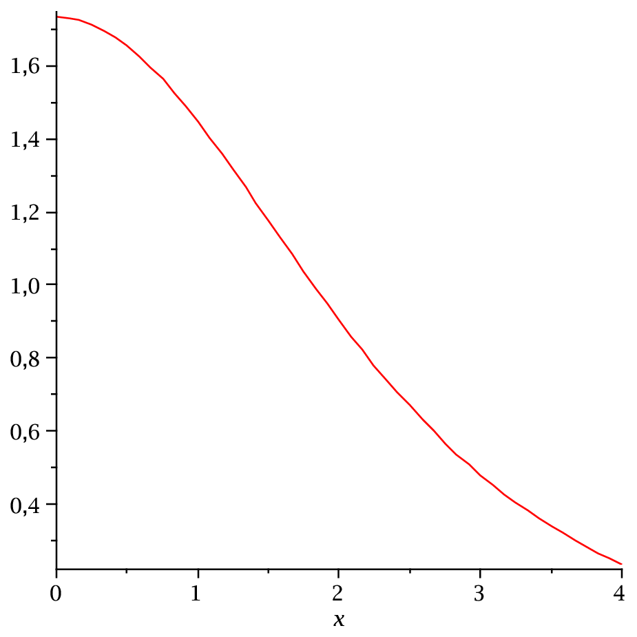
This is an stable potential, with spontaneous symmetry breaking minima, where the scalar field interpolates smoothly between that in fact is the same point due to the odd parity of coordinate. This is an AdS spacetime with cosmological constant as could be seen from and Fig.1.


Here we will present another two new solutions, these are found by setting:
| (34) | |||||
| (35) |
using (26) we get , and setting as before, we obtain the metric ”warped” factors, respectively
| (36) | |||||
| (37) |
From (24) we obtain the potential and solving r as a function of f as before we get the potentials, respectively
| (38) | |||||
| (39) |
The potentials (38) and (39) with the metrics warped factors (36) and (37), that corresponds to the scalar ”kink” fields (34) and (35) are very similar in shape to the former solution (33),(30) and (28) plotted in Fig.1. As before the potentials presents symmetry breaking minima, and the scalar field is also an interpolating soliton between those minima in AdS space time with cosmological constant and , respectively.
Remarkably these string-vortex solutions are exact solutions with integer winding number and finite 4 dimensional energy density, integrating (16) over the extra dimensions due to the decaying warping factor (30,36,37), as could be saw in Fig.1. Note that the potential (38) is a quartic polynomial potential and could be considered as the first known exact solution to the Abelian Higgs model with a mexican hat potential.
Until now, almost all known solutions in 6D curved space-time were asymptotical or numerical [5][10] with the only exception of the one in [19] and the critical string limit [17][18][20]. If we set in (23,24,25) we obtain in concordance with the result in [19]. In general the kind of solutions we had found, are very important to establish the possibility of confinement, quantization and stability of other fields as fermions, photons, gravitons, etc., opening the possibility to further developments.
III Localized gravity on the topological string-vortex
Next, we will show that these new vortices can confine gravity. In the previous section we found an exact solution to the Einstein equations for the metric (2,22,30) for the case that the gauge field and scalar field are given by (3,4,5,610,28) with the non trivial potential (33). We will study linearized spin 2 metric fluctuations from the metric (30) neglecting graviscalar and graviphotons modes.
| (40) |
where stands for the cordinates on the 4 dimensional branes and for the polar coordinates of the bulk. These massive modes (40) obeys the Laplace Beltrami operator, and straightforward the radial modes satisfy [24]
| (41) |
where represents the mass of mode with square 4 dimensional momentum . The mass term takes into account the contributions from orbital angular momentum , as in [10] while due it takes into account the contribution of the (plus) radial momentum square.
Upon substitution of (22,30) we get the equation for massive metric fluctuations:
| (42) |
when the equation (42) reduces to:
| (43) |
integrating (43), we obtain the massless mode
| (44) |
with integrations constants and .
As is monotonous growing, we must fix , in order to render normalizable. That is consistent with the boundary conditions
| (45) |
that allows (41) to be a self adjoint Sturm-Liouville well possed problem [10].
The ortonormalization condition to be satisfied by is
| (46) | |||||
so the equivalent wavefunction in 1-dimensional quantum mechanics is
| (47) |
Finally, the massless normalized equivalent wavefunction is given by:
| (48) |
This function is strongly decaying (see Fig.2), so we conclude that the massless, spin two, gravitation mode is localized on the 3-brane and strongly concentrated around as we expected for a RS scenario [5][10].
There is another approach to study the localization of gravity modes around the vortex [25][26] in an exact way, the equation (42) could be written as
| (49) |
that could be converted with the change of variables
| (50) |
into a 1 dimensional stationary Schrödinger equation with zero eingënvalue:
| (51) |
here
| (52) |
Note by squaring and integrating (50) that if is a bounded state, then is also bounded.


For the case of solution(30), the quantum potential for massive states is:
| (53) |
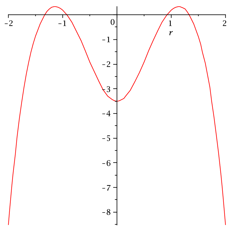
Due to the negative term in the first term in the quantum potential (53), there will be not bounded states except for , as could be seen from Fig.3. When the potential is not bounded from below, as could be observed from Fig.4 so the potential well is unstable and the massive states will easily tunnel outside the well. Therefore only the massless state will be bounded.
In a similar way the equivalent quantum mechanical potential for the other two vortex solutions (34,36) and (35,37) could easily be obtained from equation (52), we can again observe in Fig.3 that when , there exist a potential well that allows the existence of a confined massless gravity ground state, but when , the potential has a negative exponential growing, as could be seen in Fig.4, so is not bounded from below and massive bounded states are forbidden.


IV Massive gravity modes and newtonian limit of gravity.
In order to compute the newtonian limit of gravity we need exact solutions to massive modes equation (42). This equation can be solved for particular values of in term of Heun confluent functions [27]:
For we get for :
| (54) |
while for we get for :
| (55) | |||
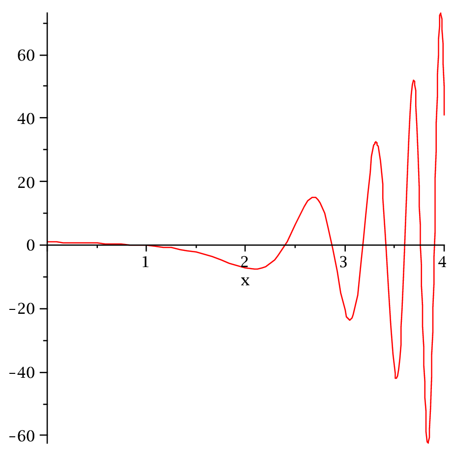
A plot of the massive wavefunction (47) is given in Fig. (5) when and using (54). In that figure its oscillating growing nature could be observed.
Although general wavefunction solutions are rather cumbersome, what really matters is the asymptotic behavior of the massive modes. Far from the vortex core or equivalently for that correspond to the thin string limit, we can approximate (30) by
| (56) |
for the other two vortices (34,36) and (35,37), we were not able to found exact solutions to equation (41), but we can obtain the same asymptotic limit (56) for the second exact solution (36) with and and for the third exact solution (37) if we set and . So the massive wavefunction (42) could be approximate for all these three vortex solutions by
| (57) |
and the localized zero mode is given by
| (58) |
The massless zero mode is then localized in the vicinity of , that means that massless gravitons, that mediates ”normal” 4D gravity, could only be found near the 3 brane where the known universe is located, decaying exponentially in number when when is increased, while far from the 3-brane only could be found as seen from Fig.5 showing the behavior of the massive wave functions.
Using the approximation (56) and (57) into the differential equation (42), and taking the limit for which we obtain
which solution is given in term of bessel functions and . In exact concordance with the result in [10].
The newtonian limit was obtained in [10], using a radial cutoff approach calculation as:
| (59) |
where is the 4 dimensional Planck mass, and is the distance between two particles of masses and on the 3-brane. Therefore the correction to the newtonian gravity decays stronger than correction in 5 dimensional RS domain walls [2] due to the additional dimension and in the thin string limit the correction to the newtonian potential vanishes.
V Summary and outlook
We consider the central result of this paper, is to have found exact topological solutions embedded in curved 6D spacetime that localize gravity. These solutions, were obtained following the procedure developed in [21] and [22] to obtain solutions to Einstein equations with proposed scalars kinks sources for suitable scalar potentials. These topological solutions corresponds to different electromagnetic field vacua and are, in fact, string-vortices in 6D with non trivial winding number.
We found three new exact 6D vortex solutions, for three different kinks, that renders adequate warped metric factors and potentials with degenerate minima that allows spontaneous symmetry breaking of the theory. The first solution (28), (30) and (33) is the vortex version of the domain wall solution in [23] where could be seen as the string thickness and as a parameter depending on the cosmological constant. The second solution (34), (36) and (38) has a quartic polynomial potential that is almost identical to the mexican hat potential. The third solution (35), (37) and (39) combine polynomial and not polynomial terms in the potential. All the new solutions presented here, are very similar to the domain walls, but the new solutions includes axial symmetry in 6 dimension and a gauge background with integer winding number, that is absent in 5 dimensional domain walls.
As expected for a RS brane world, we have shown that the zero mode (44) of the linearized gravity spectrum is localized on the 3-brane while the massive modes (47,54) are not bounded at all. The results of section III were obtained for the 6D topological vortex solutions without approximations. The newtonian limit was also obtained in complete concordance with known results [10].
Using exact solutions many interesting properties of 6D brane world could be study. If we use these topological vortex solutions as background, we can proceed to study the quantization and stability under fluctuations, it is also possible to study the confinement of electromagnetic spin 1 and other gauge or fermionic fields in an exact way. These subjects are currently under research [28].
Acknowledgments
This work was supported by CDCHT-UCLA under project 005-CT-2007.
References
- [1] L. Randall and R. Sundrum, Phys. Rev. Lett. 83, 3370 (1999) [arXiv:hep-ph/9905221].
- [2] L. Randall and R. Sundrum, Phys. Rev. Lett. 83, 4690 (1999) [arXiv:hep-th/9906064].
- [3] B. Bjac, G. Gabadadz´e, Phys. Lett. B 474 (2000) 282; M. Gremm, Phys. Lett. B 478, 434 (2000) [arXiv:hep-th/9912060]; C. Ringeval, P. Peter, J.-P. Uzan.Phys.Rev. D65 (2002) 044016; Minoru Eto, Nobuhito Maru, Norisuke Sakai.Nucl.Phys. B673 (2003) 98-130.
- [4] W. Naylor and M. Sasaki, Prog. Theor. Phys. 113, 535 (2005) [arXiv:hep-th/0411155]. M. Minamitsuji, W. Naylor and M. Sasaki, Nucl. Phys. B 737, 121 (2006) [arXiv:hep-th/0508093]. J. Garriga, O. Pujolas and T. Tanaka, Nucl. Phys. B 655, 127 (2003) [arXiv:hep-th/0111277]. A. Flachi and D. J. Toms, Nucl. Phys. B 610, 144 (2001) [arXiv:hep-th/0103077].
- [5] M. Giovannini, H. Meyer and M. E. Shaposhnikov, Nucl. Phys. B 619, 615 (2001) [arXiv:hep-th/0104118].
- [6] E. Roessl and M. Shaposhnikov, Phys. Rev. D 66, 084008 (2002) [arXiv:hep-th/0205320].
- [7] E. R. Bezerra de Mello and B. Hartmann, Phys. Lett. B 639, 546 (2006) [arXiv:hep-th/0603077].
- [8] I. Olasagasti and A. Vilenkin, Phys. Rev. D 62, 044014 (2000) [arXiv:hep-th/0003300].
- [9] N. Arkani-Hamed, S. Dimopoulos and G. R. Dvali, Phys. Lett. B 429, 263 (1998) [arXiv:hep-ph/9803315]; I. Antoniadis, N. Arkani-Hamed, S. Dimopoulos and G. R. Dvali, Phys. Lett. B 436, 257 (1998) [arXiv:hep-ph/9804398].
- [10] T. Gherghetta and M. E. Shaposhnikov, Phys. Rev. Lett. 85, 240 (2000) [arXiv:hep-th/0004014].
- [11] S. Randjbar-Daemi, M. Shaposhnikov, Phys. Lett. B 492 (2000) 361.[arXiv:hep-th/0008079
- [12] M. Giovannini, Phys. Rev. D 66, 044016 (2002) [arXiv:hep-th/0205139].
- [13] M. Giovannini, J. V. Le Be and S. Riederer, Class. Quant. Grav. 19, 3357 (2002) [arXiv:hep-th/0205222].
- [14] S. Randjbar-Daemi and M. Shaposhnikov, Nucl. Phys. B 645, 188 (2002) [arXiv:hep-th/0206016].
- [15] S. Randjbar-Daemi and M. Shaposhnikov, JHEP 0304, 016 (2003) [arXiv:hep-th/0303247]. S. L. Parameswaran, S. Randjbar-Daemi and A. Salvio, Nucl. Phys. B 767, 54 (2007) [arXiv:hep-th/0608074].
- [16] H.B. Nielsen and P. Olesen,Nucl. Phys. B 61, 45 (1973).
- [17] Bogomol’nyi E. B.Sov. J. Nucl. Phys. 24, 449 (1976).
- [18] de Vega and Schaposnik, F. A.Phys. Rev. D 14, 1100 (1976)
- [19] Y. Brihaye, T. Delsate and B. Hartmann, Phys. Rev. D 74, 044015 (2006) [arXiv:hep-th/0602172].
- [20] J. Preskill, Les Houches Summer School, Les Houches, France (1985).
- [21] R. Guerrero, R. Ortiz, R. O. Rodriguez and R. S. Torrealba, Gen. Rel. Grav. 38, 845 (2006) [arXiv:gr-qc/0504080].
- [22] R. Guerrero, R. O. Rodriguez and R. S. Torrealba, Phys. Rev. D 72, 124012 (2005) [arXiv:hep-th/0510023].
- [23] A. Melfo, N. Pantoja and A. Skirzewski, Phys. Rev. D 67, 105003 (2003) [arXiv:hep-th/0211081].
- [24] G. V. Lavrelasvili and P. G. Tinyakov, Sov. J. Nucl. Phys. 41 (1985) 172
- [25] O. Castillo-Felisola, A. Melfo, N. Pantoja and A. Ramirez, Phys. Rev. D 70, 104029 (2004) [arXiv:hep-th/0404083].
- [26] A. Wang, Phys. Rev. D 66, 024024 (2002) [arXiv:hep-th/0201051].
- [27] Tao Ma and Shu-Min Li, [arXiv:cond-mat.other/0711.1458]
- [28] In preparation.