Tailored mixing inside a translating droplet

We consider a spherical Newtonian drop immersed in an incompressible Newtonian flow in the case where the linear external field is characterized by translational velocity and vorticity vectors, similarly to [12]. As in the latter reference, we assume that the local Re is much smaller than one and that the interfacial tension is sufficiently large for the drop to remain spherical.
The internal velocity field is obtained by solving the Stokes flow problem for both the internal and external flows satisfying the continuity of velocity and tangential stress conditions across the drop surface. In addition, we introduce unsteadiness in the problem by making the vorticity time dependent. In a Cartesian coordinate system translating with the center-of-mass velocity of the drop, and with the $z$ axis in the direction of the translation, the paths of passive marker particles are given by the solution of the non-autonomous dynamical system:

where all lengths and velocities have been non-dimensionalized by the drop radius and the magnitude of the translational velocity. Here, the vorticity is defined by $\bm{\omega}=(\omega_{x},\omega_{y},\omega_{z})=(1/\sqrt{2},0,1/\sqrt{2})$, the unitary vector corresponding to the axis of rotation, and $a(t)=\varepsilon/2\left(1+\cos\omega t\right)$, characterized by the frequency $\omega$ and the amplitude $\varepsilon$. In this letter, we consider only small amplitudes, i.e. for $0\leq\varepsilon\ll 1$. Note that the former equations are identical to those in [12] except that the constant vorticity vector has been replaced by $a(t)\bm{\omega}$. This can be done by either assuming unsteady vorticity in the external flow field, or by applying a time dependent body force. In practice, this could be realized, e.g., by creating a time dependent swirl motion in the external flow or by applying an electric field that exerts a torque on the drop (e.g.,[25] it or work on electrorotation). This flow is the superposition of a Hill’s vortex and an unsteady rigid body rotation, and the surface of the drop, $r^{2}=x^{2}+y^{2}+z^{2}=1$, is invariant under flow (1).

We now discuss some features of the unperturbed axisymmetric (2D) flow ($\varepsilon=0$). The flow possesses two independent integrals of motion, e.g., the streamfunction $\psi$ and the azimuthal angle $\phi$:

where $\rho^{2}=x^{2}+y^{2}$ and $\psi\in\left[0,1/8\right]$. The streamlines of the unperturbed system are lines of constant $\psi$ and $\phi$, denoted by $\Gamma_{\psi,\phi}$, and defined as $(1-2\rho^{2})^{2}+(2\rho z)^{2}=1-8\psi$ (see Fig. 1). Almost all streamlines are closed curves surrounding a circle of degenerate elliptic fixed points $(\rho=1/\sqrt{2},z=0)$. In addition, there are two hyperbolic fixed points located at the poles of the sphere which are connected by heteroclinic orbits. The frequency of the motion on $\Gamma_{\psi,\phi}$ is given by

where $\gamma(\psi)=\sqrt{1-8\psi}$ and $K$ is the complete elliptic function of the first kind. The frequency $\Omega$ is bounded by two limits, $\Omega(0)=0$ and $\Omega(1/8)=\sqrt{2}$ (see Fig. 1).

On every streamline $\Gamma_{\psi,\phi}$, we introduce a uniform phase $\chi~\mbox{ mod}(2\pi)$ such that $\chi=0$ on the $x-y$ plane (with $\rho\leq 1/\sqrt{2}$) and $\dot{\chi}=\Omega\left(\psi\right)$. The unperturbed system, which can be rewritten in terms of $(\psi,\phi,\chi)$ as

belongs to the class of action-action-angle flows.

In the perturbed case $0<\varepsilon\ll 1$, the time evolution of the two invariants of the unperturbed system is given by

where $G(\psi,\chi)=z/\rho$ is $2\pi$ periodic in $\chi$ and has zero average in $\chi$. The time evolution equation for $\chi$ is

where $H$ is $2\pi$ periodic in $\chi$. The dynamics possesses two time scales, a fast one (of order one) associated with $\chi$, and a slow one (of order $1/\varepsilon$) associated with $\psi$ and $\phi$.
If $\Omega$ and $\omega$ are incommensurate, then the averaging over $\Omega$ and over $\omega$ can be performed independently. In this case, the time-periodic terms in Eq. (4) average out, and the averaged system reduces to $\dot{\psi}=0,\quad\dot{\phi}=-\varepsilon/2$. Thus in the averaged system the value of $\psi$ is conserved as it was in the unperturbed system; in other words, $\psi$ is an invariant of the averaged system. Each trajectory of the averaged system evolves on two-dimensional nested tori ${\mathcal{T}}_{\psi}$. In the perturbed system, $\psi$ is an adiabatic invariant and the motion follows adiabatically the tori ${\mathcal{T}}_{\psi}$.

We now turn to the generation of a 3D chaotic mixing region inside the drop, for which we seek to control both the location and the size. The strategy used for this purpose is to bring a chosen family of unperturbed tori ${\mathcal{T}}_{\psi}$ into resonance with the perturbation $a(t)$ by adjusting the frequency $\omega$ to satisfy the resonance condition

for some $n\in\mathbb{N}$ (see Fig. 1). For any fixed $\omega$ we denote by $\left\{{\mathcal{T}}^{(n)}(\omega)~|n\in\mathbb{N}\right\}$ the set of resonant tori ${\mathcal{T}}_{\psi}$ satisfying (5). Hereafter, we denote the chaotic mixing region generated around ${\mathcal{T}}^{(1)}(\omega)$ by CMR.

Figures 2 and  3 present Liouvillian sections of the perturbed system, which consist of 2D projections of time-periodic 3D flows by a combination of a stroboscopic map and a Poincaré section (here, the $y=0$ plane). Figure 2 shows that a perturbation $a(t)$ creates a 3D CMR around ${\mathcal{T}}^{(1)}(\omega)$ and its location is controlled by varying $\omega$ according to Eq. (5). In what follows, we analyze the location and the size of the CMR as $\omega$ and $\varepsilon$ vary.

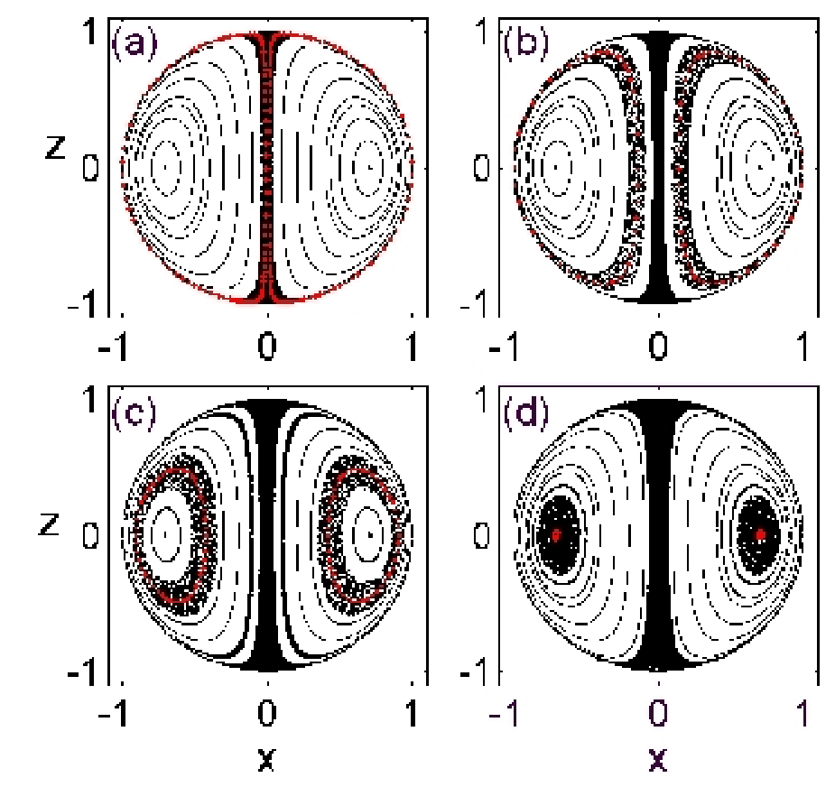
For small values of $\omega$, all resonances are located near the pole-to-pole heteroclinic connections (at $\psi=0$, near the $z$ axis and near the boundaries of the drop, see Fig. 2a). As $\omega$ is increased, the CMR penetrates deeper into the drop (Fig. 2b). In the interval $0<\omega<\sqrt{2}$, the CMR is the largest chaotic region (compared to chaotic regions corresponding to higher order resonances), with all the other chaotic regions localized close to the $z$ axis and near the drop boundaries (around the heteroclinic orbits); this is due to the shape of $\Omega\left(\psi\right)$. As $\omega$ is increased further, the CMR moves toward the location of the elliptic fixed points of the unperturbed system, closely following the location of the resonant torus ${\mathcal{T}}^{(1)}(\omega)$ (Fig. 2c). As the value of $\omega$ approaches $\sqrt{2}$, the CMR shrinks to the circle of elliptic fixed points (Fig. 5).

Whereas the frequency $\omega$ of the rigid body rotation is mostly responsible for the location of the CMR, it is its amplitude $\varepsilon$ which mostly determines its size. Figure 3 shows that the size of the chaotic mixing regions created by the $n=1$ resonance and by higher order resonances (mostly the $n=2$ resonance) increases as the amplitude of the perturbation increases. Around $\varepsilon\approx 0.20$, the chaotic regions around the heteroclinic orbits and the CMR join together to cover the entire drop volume.

Recall that in the averaged system the adiabatic invariant $\psi$ is constant. In the exact system, however, along a given trajectory starting at $\psi=\psi_{0}$ it varies between $\psi^{-}\left(\psi_{0};\omega,\varepsilon\right)$ and $\psi^{+}\left(\psi_{0};\omega,\varepsilon\right)$. The width $\Delta\psi=\psi^{+}\left(\psi_{0};\omega,\varepsilon\right)-\psi^{-}\left(\psi_{0};\omega,\varepsilon\right)$ is small away from the resonance, and increases significantly closer to the resonance. The projection of three characteristic trajectories onto the $(\psi,\phi)$-plane (called the slow plane in dynamical systems) is presented in Fig. 4. The narrow regions on the sides are off-resonance trajectories that stay quite close to the corresponding tori ${\mathcal{T}}_{\psi}$. In between, the middle trajectory deviates much further from its ${\mathcal{T}}_{\psi}={\mathcal{T}}^{(1)}(\omega)$ and fills the entire CMR. The quantity $\Delta\psi$ is probably the most convenient quantity to estimate the size of the CMR (around ${\mathcal{T}}^{(1)}(\omega)$ for $\omega<\sqrt{2}$). The volume between the tori ${\mathcal{T}}_{\psi^{-}}(\omega)$ and ${\mathcal{T}}_{\psi^{+}}(\omega)$ gives the CMR size in 3D.
The dependence of the size of the CMR (in terms of $\Delta\psi$) on $\varepsilon$ and $\omega$ is illustrated in Fig. 5. The curves (a)-(d) in the upper and lower panels correspond to the Figs. 2a-d and  3a-d, respectively. For a given $\omega$ value (i.e. for a given ${\mathcal{T}}^{(1)}(\omega)$), the size can be controlled by adjusting the value of $\varepsilon$; for example in the range of frequencies $1.181\leq\omega\leq 1.357$, the entire droplet exhibits chaotic mixing for $\varepsilon\geq 0.175$. For each smaller value of $\varepsilon$ the size reaches a maximum for a certain value $\omega^{m}\left(\varepsilon\right)$ of the frequency. On the one hand, this property can be used as an optimization technique to obtain the maximal CMR size one can reach for a given amplitude $\varepsilon$ of the rotation. On the other hand, $\Delta\psi$ versus $\varepsilon$ increases quite monotonically for all values of $\omega$. The derivation of the maxima locations and estimates of $\Delta\psi$ as functions of the parameters and the order of resonance, will be addressed elsewhere. The structure of the CMR in our case is rather different from that obtained in other problems that possess resonance-induced chaotic advection. Namely, here the size of the CMR vanishes as $\varepsilon$ goes to $0$ and the CMR is localized near the resonance. In contrast, in the flow considered in, e.g., [17], the mixing is caused by resonances, but the CMR occupies a volume on the scale of the whole system. The difference comes from the fact that the averaged change of the frequency of the fast system vanishes in the current system, thus preventing the trajectories starting away from the resonance from approaching it. This property makes the kind of flows investigated here useful as it may be advantageous to localize the mixing in certain parts of the system only.