A compact topology for Sand Automata Thanks: This work has been supported by the Interlink/MIUR project “Cellular Automata: Topological Properties, Chaos and Associated Formal Languages”, by the ANR Blanc “Projet Sycomore” and by the PRIN/MIUR project “Formal Languages and Automata: Mathematical and Applicative Aspects”.Thanks: Some of the results of this paper have been submitted at JAC 2008 and IFIP TCS 2008 conferences.
Abstract
In this paper, we exhibit a strong relation between the sand automata configuration space and the cellular automata configuration space. This relation induces a compact topology for sand automata, and a new context in which sand automata are homeomorphic to cellular automata acting on a specific subshift. We show that the existing topological results for sand automata, including the Hedlund-like representation theorem, still hold. In this context, we give a characterization of the cellular automata which are sand automata, and study some dynamical behaviors such as equicontinuity. Furthermore, we deal with the nilpotency. We show that the classical definition is not meaningful for sand automata. Then, we introduce a suitable new notion of nilpotency for sand automata. Finally, we prove that this simple dynamical behavior is undecidable.
Keywords: sand automata, cellular automata, dynamical systems, subshifts, nilpotency, undecidability
1 Introduction
Self-organized criticality (SOC) is a common phenomenon observed in a huge variety of processes in physics, biology and computer science. A SOC system evolves to a “critical state” after some finite transient. Any perturbation, no matter how small, of the critical state generates a deep reorganization of the whole system. Then, after some other finite transient, the system reaches a new critical state and so on. Examples of SOC systems are: sandpiles, snow avalanches, star clusters in the outer space, earthquakes, forest fires, load balance in operating systems [2, 5, 4, 3, 20]. Among them, sandpiles models are a paradigmatic formal model for SOC systems [11, 12].
In [6], the authors introduced sand automata as a generalization of sandpiles models and transposed them in the setting of discrete dynamical systems. A key-point of [6] was to introduce a (locally compact) metric topology to study the dynamical behavior of sand automata. A first and important result was a fundamental representation theorem similar to the well-known Hedlund’s theorem for cellular automata [13, 6]. In [7, 8], the authors investigate sand automata by dealing with some basic set properties and decidability issues.
In this paper we continue the study of sand automata. First of all, we introduce a different metric on configurations (i.e. spatial distributions of sand grains). This metric is defined by means of the relation between sand automata and cellular automata [8]. With the induced topology, the configuration set turns out to be a compact (and not only locally compact), perfect and totally disconnected space. The “strict” compactness gives a better topological background to study the behavior of sand automata (and in general of discrete dynamical systems). In fact, compactness provides a lots of very useful results which help in the investigation of several dynamical properties [1, 16]. We show that all the topological results from [6] still hold, in particular the Hedlund-like representation theorem remains valid with the compact topology. Moreover, with this topology, any sand automaton is homeomorphic to a cellular automaton defined on a subset of its usual domain. We prove that it is possible to decide whether a given cellular automaton is in fact a sand automaton. Besides, this relation helps to prove some properties about the dynamical behavior of sand automata, such as the equivalence between equicontinuity and ultimate periodicity.
Then, we study nilpotency of sand automata. The classical definition of nilpotency for cellular automata [10, 14] is not meaningful, since it prevents any sand automaton from being nilpotent. Therefore, we introduce a new definition which captures the intuitive idea that a nilpotent automaton destroys all the configurations: a sand automaton is nilpotent if all configurations get closer and closer to a uniform configuration, not necessarily reaching it. Finally, we prove that this behavior is undecidable.
The paper is structured as follows. First, in Section 2, we recall basic definitions and results about cellular automata and sand automata. Then, in Section 3, we define a compact topology and we prove some topological results, in particular the representation theorem. Finally, in Section 4, nilpotency for sand automata is defined and proved undecidable.
2 Definitions
For all with , let and . For , let . Let be the set of positive integers. For a vector , denote by the infinite norm of .
Let a (possibly infinite) alphabet and . Denote by the set of all the -dimensional matrices with values in . We assume that the entries of any matrix are all the integer vectors of a suitable -dimensional hyper-rectangle . For any , let be the set of all the matrices with entries in . In the sequel, the vector will be called the order of the matrices belonging to . For a given element , the finite portion of of reference position and order is the matrix defined as , . For any , let (or simply if the dimension is not ambiguous) be the vector .
2.1 Cellular automata and subshifts
Let be a finite alphabet. A CA configuration of dimension is a function from to . The set of all the CA configurations is called the CA configuration space. This space is usually equipped with the Tychonoff metric defined by
The topology induced by coincides with the product topology induced by the discrete topology on . With this topology, the CA configuration space is a Cantor space: it is compact, perfect (i.e., it has no isolated points) and totally disconnected.
For any the shift map is defined by , . A function is said to be shift-commuting if , .
A -dimensional subshift is a closed subset of the CA configuration space which is shift-invariant, i.e. for any , . Let and let be the set of configurations such that all possible finite portions of do not belong to , i.e. for any , . The set is a subshift, and is called its set of forbidden patterns. Note that for any subshift , it is possible to find a set of forbidden patterns such that . A subshift is said to be a subshift of finite type (SFT) if for some finite set . The language of a subshift is (for more on subshifts, see [17] for instance).
A cellular automaton is a quadruple , where is the alphabet also called the state set, is the dimension, is the radius and is the local rule of the automaton. The local rule induces a global rule defined as follows,
Note that CA are exactly the class of all shift-commuting functions which are (uniformly) continuous with respect to the Tychonoff metric (Hedlund’s theorem from [13]). For the sake of simplicity, we will make no distinction between a CA and its global rule .
The local rule can be extended naturally to all finite matrices in the following way. With a little abuse of notation, for any and any , define as the matrix obtained by the simultaneous application of to all the submatrices of . Formally, , where is any configuration such that .
For a given CA, a state is quiescent (resp., spreading) if for all matrices such that , (resp., ) , it holds that . Remark that a spreading state is also quiescent. A CA is said to be spreading if it has a spreading state. In the sequel, we will assume that for every spreading CA the spreading state is .
2.2 SA Configurations
A SA configuration (or simply configuration) is a set of sand grains organized in piles and distributed all over the -dimensional lattice . A pile is represented either by an integer from (number of grains), or by the value (source of grains), or by the value (sink of grains), i.e. it is an element of . One pile is positioned in each point of the lattice . Formally, a configuration is a function from to which associates any vector with the number of grains in the pile of position . When the dimension is known without ambiguity we note the null vector of . Denote by the set of all configurations. A configuration is said to be constant if there is an integer such that for any vector , . In that case we write . A configuration is said to be bounded if there exist two integers such that for all vectors , . Denote by the set of all bounded configurations.
A measuring device of precision and reference height is a function from to defined as follows
A measuring device is used to evaluate the relative height of two piles, with a bounded precision. This is the technical basis of the definition of cylinders, distances and ranges which are used all along this article.
In [6], the authors equipped with a metric in such a way that two configurations are at small distance if they have the same number of grains in a finite neighborhood of the pile indexed by the null vector. The neighborhood is individuated by putting the measuring device at the top of the pile, if this latter contains a finite number of grains. Otherwise the measuring device is put at height . In order to formalize this distance, the authors introduced the notion of cylinder, that we rename top cylinder. For any configuration , for any , and for any , the top cylinder of centered in and of radius is the -dimensional matrix defined on the infinite alphabet by
In dimension and for a configuration , we have
if , while
if .
By means of top cylinders, the distance has been introduced as follows:
2.3 Sand automata
For any integer , for any configuration and any index with , the range of center and radius is the -dimensional matrix on the finite alphabet such that
The range is used to define a sand automaton. It is a kind of top cylinder, where the observer is always located on the top of the pile (called the reference). It represents what the automaton is able to see at position . Sometimes the central symbol may be omitted for simplicity sake. The set of all possible ranges of radius , in dimension , is denoted by .
A sand automaton (SA) is a deterministic finite automaton working on configurations. Each pile is updated synchronously, according to a local rule which computes the variation of the pile by means of the range. Formally, a SA is a triple , where is the dimension, is the radius and is the local rule of the automaton. By means of the local rule, one can define the global rule as follows
Remark that the radius of the automaton has three different meanings: it represents at the same time the number of measuring devices in every dimension of the range (number of piles in the neighborhood), the precision of the measuring devices in the range, and the highest return value of the local rule (variation of a pile). It guarantees that there are only a finite number of ranges and return values, so that the local rule has finite description.
The following example illustrates a sand automaton whose behavior will be studied in Section 4. For more examples, we refer to [8].
[the automaton ] This automaton destroys a configuration by collapsing all piles towards the lowest one. It decreases a pile when there is a lower pile in the neighborhood (see Figure 1). Let of global rule where

When no misunderstanding is possible, we identify a SA with its global rule . For any , we extend the definition of the shift map to , is defined by , . The raising map is defined by , . A function is said to be vertical-commuting if . A function is infinity-preserving if for any configuration and any vector , if and only if and if and only if .
Remark that the raising map is the sand automaton of radius whose local rule always returns . On the opposite, the horizontal shifts are not sand automata: they destroy infinite piles by moving them, which is not permitted by the definition of the global rule.
3 Topology and dynamics
In this section we introduce a compact topology on the SA configuration space by means of a relation between SA and CA. With this topology, a Hedlund-like theorem still holds and each SA turns out to be homeomorphic to a CA acting on a specific subshift. We also characterize CA whose action on this subshift represents a SA. Finally, we prove that equicontinuity is equivalent to ultimate periodicity, and that expansivity is a very strong notion: there exist no positively expansive SA.
3.1 A compact topology for SA configurations
From [8], we know that any SA of dimension can be simulated by a suitable CA of dimension (and also any CA can be simulated by a SA). In particular, a -dimensional SA configuration can be seen as a ()-dimensional CA configuration on the alphabet . More precisely, consider the function defined as follows
A SA configuration is coded by the CA configuration . Remark that is an injective function.
Consider the -dimensional matrix such that and . With a little abuse of notation, denote the subshift of configurations that do not contain the pattern .
Proposition 3.1
The set is the subshift .
Proof. Each -dimensional SA configuration is coded by the -dimensional CA configuration such that for any , then . Conversely, we can define a preimage by for any , by . Hence .
Figure 2 illustrates the mapping and the matrix for the dimension . The set of SA configurations can be seen as the subshift of the CA configurations set .


Definition 3.1
The distance is defined as follows:
In other words, the (well defined) distance between two configurations is nothing but the Tychonoff distance between the configurations in the subshift . The corresponding metric topology is the product topology induced on .
Remark 1
Note that this topology does not coincide with the topology obtained as countable product of the discrete topology on . Indeed, for any , the projection defined by is not continuous in any configuration with . However, it is continuous in all configurations such that , since , conditions and imply that .
By definition of this topology, if one considers as a map from onto , turns out to be an isometric homeomorphism between the metric spaces (endowed with ) and (endowed with ). As an immediate consequence, the following results hold.
Proposition 3.2
The set is a compact and totally disconnected space where the open balls are clopen (i.e. closed and open) sets.
Proposition 3.3
The space is perfect.
Proof. Choose an arbitrary configuration . For any , let such that . We build a configuration , equal to except at site , defined as follows
By Definition 3.1, .
Consider now the following notion.
Definition 3.2 (ground cylinder)
For any configuration , for any , and for any , the ground cylinder of centered on and of radius is the -dimensional matrix defined by
For example in dimension ,
Figure 3 illustrates top cylinders and ground cylinders in dimension . Remark that the content of the two kinds of cylinders is totally different.

.

.
From Definition 3.1, we obtain the following expression of distance by means of ground cylinders.
Remark 2
For any pair of configurations , we have
As a consequence, two configurations are compared by putting boxes (the ground cylinders) at height around the corresponding piles indexed by . The integer is the size of the smallest cylinders in which a difference appears between and . This way of calculating the distance is similar to the one used for the distance , with the difference that the measuring devices and the cylinders are now located at height . This is slightly less intuitive than the distance , since it does not correspond to the definition of the local rule. However, this fact is not an issue all the more since the configuration space is compact and the representation theorem still holds with the new topology (Theorem 3.5).
3.2 SA as CA on a subshift
Let and be two metric spaces. Two functions , are (topologically) conjugated if there exists a homeomorphism such that .
We are going to show that any SA is conjugated to some restriction of a CA. Let a -dimensional SA of radius and local rule . Let us define the ()-dimensional CA on the alphabet , with radius and local rule defined as follows (see [8] for more details). Let be a matrix on the finite alphabet which does not contain the pattern . If there is a such that and , then let be the range taken from of radius centered on . See figure 4 for an illustration of this construction in dimension .

The new central value depends on the height of the central column plus its variation. Therefore, define if , if , or (central value unchanged) if there is no such .
The following diagram commutes:
| (1) |
i.e. . As an immediate consequence, we have the following result.
Proposition 3.4
Any -dimensional SA is topologically conjugated to a suitable -dimensional CA acting on .
Being a dynamical submodel, SA share properties with CA, some of which are proved below. However, many results which are true for CA are no longer true for SA; for instance, injectivity and bijectivity are not equivalent, as proved in [7]. Thus, SA deserve to be considered as a new model.
Corollary 3.3
The global rule of a SA is uniformly continuous w.r.t distance .
Proof. Let be the global rule of the CA which simulates the given SA. Since the diagram (1) commutes and is a homeomorphism, . Since is a continuous map and, by Proposition 3.2, is compact, then the thesis is obtained.
For every , let be the clopen (and compact) set of all configurations such that .
Lemma 3.4
Let be a continuous and infinity-preserving map. There exists an integer such that for any configuration we have .
Proof. Since is continuous and infinity-preserving, the set is compact and included in . From Remark 1, is continuous on the set and in particular it is continuous on the compact . Hence is a compact subset of containing no infinity, and therefore it is included in some interval , where .
Theorem 3.5
A mapping is the global transition rule of a sand automaton if and only if all the following statements hold
-
is (uniformly) continuous w.r.t the distance ;
-
is shift-commuting;
-
is vertical-commuting;
-
is infinity-preserving.
Proof. Let be the global rule of a SA. By definition of SA, is shift-commuting, vertical-commuting and infinity-preserving. From Corollary 3.3, is also uniformly continuous.
Conversely, let be a continuous map which is shift-commuting, vertical-commuting, and infinity-preserving. By compactness of the space , is also uniformly continuous. Let be the integer given by Lemma 3.4. Since is uniformly continuous, there exists an integer such that
We now construct the local rule of the automaton. For any input range , set , where is an arbitrary configuration of such that , , . Note that the value of does not depend on the particular choice of the configuration such that , . Indeed, Lemma 3.4 and uniform continuity together ensure that for any other configuration such that , , we have , since and . Thus the rule is well defined.
We now show that is the global mapping of the sand automaton of radius and local rule . Thanks to , it is sufficient to prove that for any and for any with , we have . By and , for any such that , it holds that
Since , we have by definition of
Moreover, by definition of the range, for all ,
hence , which leads to .
We now deal with the following question: given a ()-dimensional CA, does it represent a -dimensional SA, in the sense of the conjugacy expressed by diagram 1? In order to answer to this question we start to express the condition under which the action of a CA can be restricted to a subshift , i.e., (if this fact holds, the subshift is said to be -invariant).
Lemma 3.6
Let and be a CA and a subshift of finite type, respectively. The condition is satisfied iff for any and any of the same order than , it holds that .
Proof. Suppose that . Choose arbitrarily and , with and of the same order. Let containing the matrix . Since , then , and so . Conversely, if and , then there exist and with .
The following proposition gives a sufficient and necessary condition under which the action of a CA on configurations of the -invariant subshift preserves any column whose cells have the same value.
Lemma 3.7
Let be a -dimensional CA with state set and be the subshift representing SA configurations. The following two statements are equivalent:
-
for any with (resp., ) for all , it holds that (resp., ) for all .
-
for any matrix with (resp., ) and any , it holds that (resp., ).
Proof. Suppose that is true. Let be a matrix with and let be a configuration such that for all and . Since for all , and , then . Conversely, let with for all . By shift-invariance, we obtain for all .
Proposition 3.5
It is decidable to check whether a given ()-dimensional CA corresponds to a -dimensional SA.
3.3 Some dynamical behaviors
SA are very interesting dynamical systems, which in some sense “lie” between -dimensional and -dimensional CA. Indeed, we have seen in the previous section that the latter can simulate -dimensional SA, which can, in turn, simulate -dimensional CA. For the dimension , a classification of CA in terms of their dynamical behavior was given in [15]. Things are very different as soon as we get into dimension , as noted in [19, 18]. The question is now whether the complexity of the SA model is closer to that of the lower or the higher-dimensional CA.
Let be a metric space and let be a continuous application. An element is an equicontinuity point for if for any , there exists such that for all , implies that , . The map is equicontinuous if for any , there exists such that for all , implies that , . If is compact, is equicontinuous iff all elements of are equicontinuity points. An element is ultimately periodic for if there exist two integers (the preperiod) and (the period) such that . is ultimately periodic if there exist and such that . is sensitive (to the initial conditions) if there is a constant such that for all points and all , there is a point and an integer such that but . is positively expansive if there is a constant such that for all distinct points , there exists such that .
The topological conjugacy between a SA and some CA acting on the special subshift helps to adapt some properties of CA. In particular, the following characterization of equicontinuous CA can be adapted from Theorem 4 of [15].
Proposition 3.6
If is a SA, then the following statements are equivalent:
- 1.
is equicontinuous.
- 2.
is ultimately periodic.
- 3.
All configurations of are ultimately periodic for .
Proof.
32: For any and ,
let . Remark that
is the union of these closed
subsets. As is complete of nonempty interior, by the Baire
Theorem, there are integers for which the set
has nonempty interior. Hence the conjugate image
has nonempty interior too, and it can easily be
seen that it is a subshift. It is known that the only subshift
with nonempty interior is the full space; hence .
23: obvious.
21: Let be ultimately
periodic with for some , . Since are uniformly continuous maps, for any
there exists such that for all
with , it holds that , , . Since for
any is equal to some with , the map
is equicontinuous.
12: For the sake of simplicity,
we give the proof for a given one-dimensional equicontinuous SA
. Let be the global rule of the two-dimensional CA whose
action on is conjugated to . By Definition 3.1,
and since the diagram 1 commutes, the map is
equicontinuous w.r.t. . So, for , there
exists such that for all , if
, then for all ,
. Consider now configurations ,
where has either the form
or . Since every are
ultimately periodic (with preperiod and period ) and
is equicontinuous, for any and any with
, it holds that the sequence
is ultimately periodic. For any
,
let be the configuration such that ,
if and , and
otherwise. Except for the finite central region, is made by the
repetition of a finite number of matrices appearing inside
configurations . Hence, is an ultimately periodic
configuration with some preperiod and period . Then,
for any with , the sequence
is ultimately periodic with preperiod
and period . Set and
where lcm is the
least common multiple. Thus, for any configuration , we
have that . By shift-invariance, we obtain
, . Concluding, is
ultimately periodic and then is too.
In [15] is presented a classification of CA into four classes: equicontinuous CA, non equicontinuous CA admitting an equicontinuity configuration, sensitive but not positively expansive CA, positively expansive CA. This classification is no more relevant in the context of SA since the class of positively expansive SA is empty. This result can be related to the absence of positively expansive two-dimensional CA (see [19]), though the proof is much different.
Proposition 3.7
There are no positively expansive SA.
Proof. Let a SA and . Take two distinct configurations such that . By infinity-preservingness, we get , hence .
An important open question in the dynamical behavior of SA is the existence of non-sensitive SA without any equicontinuity configuration. An example for two-dimensional CA is given in [18], but their method can hardly be adapted for SA. This could lead to a classification of SA into four classes: equicontinuous, admitting an equicontinuity configuration (but not equicontinuous), non-sensitive without equicontinuity configurations, sensitive.
Another issue is the decidability of these classes. In [7], the undecidability of SA ultimate periodicity was proved on the particular subsets of finite and periodic configurations. It follows directly that equicontinuity on these subsets is undecidable. The question is still open for the whole configuration space .
4 The nilpotency problem
In this section we give a definition of nilpotency for SA. Then, we prove that nilpotency behavior is undecidable (Theorem 4.5).
4.1 Nilpotency of CA
Here we recall the basic definitions and properties of nilpotent CA. Nilpotency is among the simplest dynamical behavior that an automaton may exhibit. Intuitively, an automaton defined by a local rule and working on configurations (either or ) is nilpotent if it destroys every piece of information in any initial configuration, reaching a common constant configuration after a while. For CA, this is formalized as follows.
Remark that in a similar way to the proof of Proposition 3.6, Definition 4.1 can be restated as follows: a CA is nilpotent if and only if it is nilpotent for all initial configurations.
Spreading CA have the following stronger characterization.
Proposition 4.1 ([9])
A CA , with spreading state , is nilpotent iff for every , there exists and such that (i.e. appears in the evolution of every configuration).
The previous result immediately leads to the following equivalence.
Corollary 4.2
A CA of global rule , with spreading state , is nilpotent if and only if for all configurations , .
Recall that the CA nilpotency is undecidable [14]. Remark that the proof of this result also works for the restricted class of spreading CA.
Theorem 4.3 ([14])
For a given state , it is undecidable to know whether a cellular automaton with spreading state is nilpotent.
4.2 Nilpotency of SA
A direct adaptation of Definition 4.1 to SA is vain. Indeed, assume is a SA of radius . For any , consider the configuration defined by and for any . Since the pile of height may decrease at most by during one step of evolution of the SA, and the other piles may increase at most by , requires at least steps to reach a constant configuration. Thus, there exists no common integer such that all configurations reach a constant configuration in time . This is a major difference with CA, which is essentially due to the unbounded set of states and to the infinity-preserving property.
Thus, we propose to label as nilpotent the SA which make every pile approach a constant value, but not necessarily reaching it ultimately. This nilpotency notion, inspired by Proposition 4.2, is formalized as follows for a SA :
Remark that shall not be taken in the full state set , because allowing infinite values for would not correspond to the intuitive idea that a nilpotent SA “destroys” a configuration (otherwise, the raising map would be nilpotent). Anyway, this definition is not satisfying because of the vertical commutativity: two configurations which differ by a vertical shift reach two different configurations, and then no nilpotent SA may exist. A possible way to work around this issue is to make the limit configuration depend on the initial one:
Again, since SA are infinity-preserving, an infinite pile cannot be destroyed (nor, for the same reason, can an infinite pile be built from a finite one). Therefore nilpotency has to involve the configurations of , i.e. the ones without infinite piles. Moreover, every configuration made of regular steps (i.e. in dimension , for all , ) is invariant by the SA rule (possibly composing it with the vertical shift). So it cannot reach nor approach a constant configuration. Thus, the larger reasonable set on which nilpotency might be defined is the set of bounded configurations . This leads to the following formal definition of nilpotency for SA.
Definition 4.4 (SA nilpotency)
A SA is nilpotent if and only if
The following proposition shows that the class of nilpotent SA is nonempty.
Proposition 4.2
The SA from Example 2.3 is nilpotent.
Proof. Let , let such that for all , . Clearly, after steps, . By immediate induction, we obtain that for all there exists such that , hence .
Similar nilpotent SA can be constructed with any radius and in any dimension.
4.3 Undecidability
The main result of this section is that SA nilpotency is undecidable (Theorem 4.5), by reducing the nilpotency of spreading CA to it. This emphasizes the fact that the dynamical behavior of SA is very difficult to predict. We think that this result might be used as the reference undecidable problem for further questions on SA.
Problem Nil
instance: a SA ;
question: is nilpotent?
Theorem 4.5
The problem Nil is undecidable.
Proof. This is proved by reducing Nil to the nilpotency of spreading cellular automata. Remark that it is sufficient to show the result in dimension . Let be a spreading cellular automaton of global rule , with finite set of integer states containing the spreading state . We simulate with the sand automaton of global rule using the following technique, also developed in [8]. Let be a function which inserts markers every two cells in the CA configuration to obtain a bounded SA configuration. These markers allow the local rule of the SA to know the absolute state of each pile and behave as the local rule of the CA. To simplify the proof, the markers are put at height (see Figure 5):
This can lead to an ambiguity when all the states in the neighborhood of size are at state , as shown in the picture. But as in this special case the state is quiescent for , this is not a problem: the state is preserved, and markers are preserved.
The local rule is defined as follows, for all ranges ,
| (2) |
The first case is for the markers (and state ) which remain unchanged, the second case is the simulation of in the even piles. As proved in [8], for any it holds that . The images by of the remaining ranges will be defined later on, first a few new notions need to be introduced.
A sequence of consecutive piles from a configuration is said to be valid if it is part of an encoding of a CA configuration, i.e. (these piles are markers) and for all such that , (this is a valid state). We extend this definition to configurations, when and , i.e. for a given ( is valid if it is the raised image of a CA configuration). A sequence (or a configuration) in invalid if it is not valid.
First we show that starting from a valid configuration, the SA is nilpotent if and only if is nilpotent. This is due to the fact that we chose to put the markers at height , hence for any valid encoding of the CA , with and ,
It remains to prove that for any invalid configuration, is also nilpotent. In order to have this behavior, we add to the local rule the rules of the nilpotent automaton for every invalid neighborhood of width . For all ranges not considered in Equation (2),
| (3) |
Let be an invalid configuration. Let be any index such that , . Let be respectively the lowest and greatest indices such that and is valid ( may equal ). Remark that for all , remains valid. Indeed, the markers are by construction the lowest piles and Equations (2) and (3) do not modify them. The piles coding for non-zero states can change their state by Equation (2), or decrease it by by Equation (3), which in both cases is a valid encoding. Moreover, the piles and will reach a valid value after a finite number of steps: as long as they are invalid, they decrease by until they reach a value which codes for a valid state. Hence, by induction, for any indices , there exists such that for all the sequence is valid.
In particular, after step, there is a valid sequence of length centered on the origin (here, is the number of steps needed by to reach the configuration , given by Definition 4.1). Hence, after steps, the local rule of the CA applied on this valid sequence leads to 3 consecutive zeros at positions . All these steps are illustrated on Figure 6.
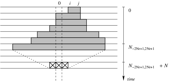
Similarly, we prove that for all , the sequence is a constant sequence which does not evolve. Therefore, there exists such that . We just proved that is nilpotent, i.e. for all , if and only if is nilpotent (because of the equivalence of definitions given by Corollary 4.2), so Nil is undecidable (Proposition 4.3).
5 Conclusion
In this article we have continued the study of sand automata, by introducing a compact topology on the SA. In this new context of study, the characterization of SA functions of [6, 8] still holds. Moreover, a topological conjugacy of any SA with a suitable CA acting on a particular subshift might facilitate future studies about dynamical and topological properties of SA, as for the proof of the equivalence between equicontinuity and ultimate periodicity (Proposition 3.6).
Then, we have given a definition of nilpotency. Although it differs from the standard one for CA, it captures the intuitive idea that a nilpotent automaton “destroys” configurations. Even though nilpotent SA may not completely destroy the initial configuration, they flatten them progressively. Finally, we have proved that SA nilpotency is undecidable (Theorem 4.5). This fact enhances the idea that the behavior of a SA is hard to predict. We also think that this result might be used as a fundamental undecidability result, which could be reduced to other SA properties.
Among these, deciding dynamical behaviors remains a major problem. Moreover, the study of global properties such as injectivity and surjectivity and their corresponding dimension-dependent decidability problems could help understand if -dimensional SA look more like -dimensional or -dimensional CA. Still in that idea is the open problem of the dichotomy between sensitive SA and those with equicontinuous configurations. A potential counter-example would give a more precise idea of the dynamical behaviors represented by SA.
References
- [1] E. Akin. The general topology of dynamical systems. Graduate Stud. Math. 1, AMS. Providence, 1993.
- [2] P. Bak. How nature works - The science of SOC. Oxford University Press, 1997.
- [3] P. Bak, K. Chen, and C. Tang. A forest-fire model and some thoughts on turbulence. Physics Letters A, 147:297–300, 1990.
- [4] P. Bak and C. Tang. Earthquakes as a self-organized critical phenomenon. Journal of Geophys. Res., 94:15635–15637, 1989.
- [5] P. Bak, C. Tang, and K. Wiesenfeld. Self-organized criticality. Physical Review A, 38(1):364–374, 1988.
- [6] J. Cervelle and E. Formenti. On sand automata. In Symposium on Theoretical Aspects of Computer Science (STACS 2003), volume 2607 of Lecture Notes in Computer Science, pages 642–653. Springer, 2003.
- [7] J. Cervelle, E. Formenti, and B. Masson. Basic properties for sand automata. In MFCS 2005, volume 3618 of Lecture Notes in Computer Science, pages 192–211. Springer, 2005.
- [8] J. Cervelle, E. Formenti, and B. Masson. From sandpiles to sand automata. Theoretical Computer Science, 381:1–28, 2007.
- [9] J. Cervelle and P. Guillon. Towards a Rice theorem on traces of cellular automata. In MFCS, volume 4708 of Lecture Notes in Computer Science, pages 310–319. Springer, 2007.
- [10] K. Culik, J. Pachl, and S. Yu. On the limit sets of cellular automata. SIAM Journal of Computing, 18(4):831–842, 1989.
- [11] E. Goles and M. A. Kiwi. Game on line graphs and sandpile automata. Theoretical Computer Science, 115:321–349, 1993.
- [12] E. Goles, M. Morvan, and H. D. Phan. Sand piles and order structure of integer partitions. Discrete Applied Mathematics, 117:51–64, 2002.
- [13] G. A. Hedlund. Endomorphisms and automorphisms of the shift dynamical system. Mathematical Systems Theory, 3:320–375, 1969.
- [14] J. Kari. The nilpotency problem of one-dimensional cellular automata. SIAM Journal of Computing, 21(3):571–586, 1992.
- [15] P. Kůrka. Languages, equicontinuity and attractors in cellular automata. Ergodic Theory & Dynamical Systems, 17:417–433, 1997.
- [16] P. Kůrka. Topological and Symbolic Dynamics. Volume 11 of Cours Spécialisés. Société Mathématique de France, 2004.
- [17] D. Lind and B. Marcus. An Introduction to Symbolic Dynamics and Coding. Cambridge University Press, 1995.
- [18] M. Sablik and G. Theyssier. Topological dynamics of 2D cellular automata. arXiv, September 2007.
- [19] M. A. Shereshevsky. Expansiveness, entropy and polynomial growth for groups acting on subshifts by automorphisms. Indag. Math., 4(2):203–210, jun 21 1993.
- [20] R. Subramanian and I. Scherson. An analysis of diffusive load-balancing. In ACM Symposium on Parallel Algorithms and Architecture (SPAA’94), pages 220–225. ACM Press, 1994.