Construction of Reversible Lattice Molecular Automata
Abstract
Several cellular automata (CA) models have been developed to simulate self-organization of multiple levels of structures. However, they do not obey microscopic reversibility and conservation laws. In this paper, we describe the construction of a reversible lattice molecular automata (RLMA) model, which simulates molecular interaction and self-organization of higher-order structures. The model’s strict reversibility entails physically relevant conservation laws, and thus opens a way to precise application and validation of the methods from statistical physics in studying the necessary conditions for such multiple levels of self-organization.
Keywords: Reversible Cellular Automata; Molecular Aggregation; Self-organization; Artificial Chemistry
1 Introduction
Possessing and utilizing multiple levels of self-organized structures—sometimes addressed as dynamical hierarchies[Rasmussen2001, McGregor2005]—is a characteristic feature of biological systems. Cellular automata (CA) and similar discrete paradigms have been effective in modeling such dynamical self-organization hierarchies. In the context of molecular aggregation, lattice molecular automata (LMA) simulates self-organization of water (polar solvent), monomers, and polymers into clusters and higher-order structures such as micelles[Mayer1997, Mayer1998, Mayer2000], and similar models have been developed to simulate organization of compartment structure and proto-cell-like self-reproduction[Ono2005, Hutton2007].
However, these models do not obey microscopic reversibility and conservation laws, and therefore, the possibility and stability of the self-organized structures in these models are, to some extent, implied in their irreversible time evolution rules. Under the laws of physics, stable persistence of an organized structure requires effective utilization of limited resources and smooth disposal of generated entropy. Therefore, the constraint of reversibility should not be omitted in studying the necessary conditions for stable structures, using, for example, the canonical methods of statistical physics.
In this paper, we describe the construction of reversible lattice molecular automata (RLMA), which simulates self-organization of water, monomers, and polymers with a strictly reversible dynamics and physically appropriate conservation laws. Although several reversible CA models have been proposed to simulate self-organization processes[Creutz1986, D'Souza1999], our model can simulate self-organization of structures with mobility, which will be essential for realizing higher-order structures and higher functionality such as autonomy.
The rest of the paper is organized as follows. A formal definition of CA is provided and useful techniques in constructing reversible CA are briefly reviewed in Section 2. Features of the original LMA model and its relation to other models are also briefly reviewed there. The construction of our RLMA model is described in Section 3, along with the conservation laws derived from the reversible dynamics. Some simulations of monomers and polymers in polar solvent are presented in Section 4. Finally, our conclusion is drawn in Section 5. Appendix A presents an alternative approach for implementing reversible molecular rotation.
2 Preliminaries
2.1 Formalization of CA
On a -dimensional spatial lattice , each site (cell) is assigned with its local state . The finite set of local states is called an alphabet. A specification of local states over the whole space is called a global state or configuration.
The dynamics of a CA is given by the local transition map as
| (1) |
where the neighbor function defines interaction range for each site . By applying the local map over the lattice, the global transition map
| (2) |
from a configuration at to the one at is derived. Although the application of over the space is synchronous in simple CA, making it asynchronous can be effective in satisfying reversibility and other constraints, as shown later. Furthermore, in more complicated CA, the local map consists not of a single map but of several maps (sub-steps), and the local states also have inner structures such as “partitions” or “layers.”
When the global transition map is bijective, that is, when for any configuration its pre-image is unique, the CA is reversible (or invertible).
2.2 Construction of reversible CA
Reversibility entails conservation of information—differences in states cannot just appear from or vanish into nowhere. Hence the manner in which to prevent information loss is crucial in constructing reversible CA.
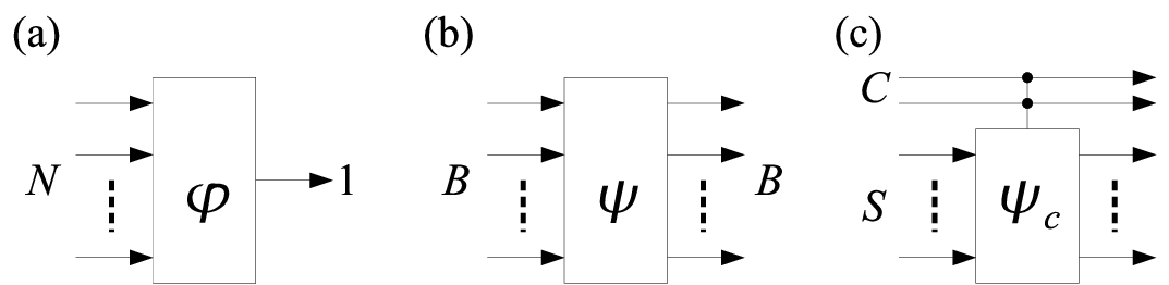
Since the many-to-one local transition map in Eq. (1) obviously loses information by itself (Fig. 1(a)), the loss should be prevented by well-counterbalanced distribution among the interacting cells. However, designing such maps is far from trivial. Indeed, judging the reversibility of a global transition map , given its corresponding local map , is a difficult task in itself.
An easier method to construct reversible CA is by adopting a permutation (reversible transformation on a finite set) ,
| (3) |
instead of a many-to-one mapping , as a constituent of the transition rule (Fig. 1(b)). Here, denotes a “block” of cells under the permutation. In Partitioning CA (or block CA)[Toffoli1990], for example, both the reversibility and global transmission of information are satisfied by combining the permutation and alternation of different partitioning schemes of a given space into cell-blocks.
The permutation (3) can be generalized into a conditional permutation as
| (4) |
Out of the set of cells that are subject to the mapping, the states of cells in work as “control signals,” which determine a permutation for the states of , and reappear unchanged as outputs (Fig. 1(c)). The Fredkin gate and the Toffoli gate are well-known examples of conditional permutations.
To prevent information loss, the outputs of the (conditional) permutations should be reused as inputs or conditional signals, and to achieve this, one needs to implement certain techniques such as dividing a time step into several sub-steps, and arranging the permutations sparsely and asynchronously in space-time[Toffoli2004].
For synchronous information transmission, one can also use global shifts, which uniformly displace some partitions or layers of local states. The translational movement of free particles can be effectively modeled by the shifts. In lattice gas automata (LGA)[Hardy1973, Frisch1986], for example, shifts are utilized to express the translation of gas particles, in combination with permutations that represent the collisions of the particles. Partitioned CA[Morita1989] is virtually equivalent to the LGA.
2.3 LMA model and other models
Various models have been proposed and used to simulate molecular self-organization processes. On the one hand, the molecular dynamics (MD) method models molecules as particles with appropriate interaction potentials, and solves their equations of motion in continuous space[Koch1983]. While the MD enables microscopically detailed description of the dynamics, size of the simulated system is restricted by the available computer resources. On the other hand, lattice-type models have been successful on simulating macroscopic behavior of phase separation and aggregation processes. Especially the Larson model[Larson1985, Larson1988, Larson1989] and its variants[Stauffer1993, Sahimi1994, Liverpool1995, Bernardes1996] are widely used and many results are reported. In the traditional Larson model simulating ternary mixture of water, oil (hydrophobic monomers), and surfactant (amphiphilic polymers), water and hydrophobic monomers are represented by a set of up and down spins, respectively, and polymers are represented by strings of spins. Monte Carlo method is used for update and the ferromagnetic interaction between the spins induces phase separation, micelle formation, etc.
The original LMA model bridges the gap between the MD method and the Larson-type models[Mayer2000]: While realized in a discrete manner and thus keeping the efficiency of the lattice setting, it includes some microscopic molecular details, such as hydrodynamics conserving momenta in the molecular collision, directions of polar molecules and accompanied anisotropy of molecular potential energy. A distinguishing feature of the LMA model is the equienergetic interaction for the pairs water–hydrophobic monomer and hydrophobic monomer–hydrophobic monomer, following experimental data on enthalpy exchanges in mixtures[Privalov1989]. This setting is in contrast to the Larson models, which define positive enthalpic gains for oil–oil interaction but not for water–oil interaction. Consequently, in the LMA model phase separation is realized via entropy-driven hydrophobic effect, and not enthalpy-driven as in the Larson-type models.
Although update rule of the LMA model partially keeps the conservation laws, its dynamics is not microscopically reversible (refer to section IV.B and V of Ref. [Mayer1997] for example to see the total energy is conserved in the mean but not strictly and explicitly). Therefore, utilizing the techniques introduced in section 2.2, we construct our RLMA model in the next section.
3 RLMA Model
3.1 Space
We formalize the RLMA model on the two-dimensional triangular lattice (Fig. 2(a), (b)) as in the literature[Mayer1997, Mayer1998], although generalization to other lattice structures and to higher dimensions will be straightforward. We use the variable to denote the principal directions, and to denote cell ’s nearest neighbor in direction , as shown in Fig. 2(c). corresponds to in the equilateral triangular lattice with a proper coordinate system (Fig. 2(c)), and on , we define a cyclic permutation of length 6,
| (5) |
which corresponds to rotation operator for the principal directions.

3.2 Local states
Each local state has the layers (internal data structure) shown in Table 1.
| Layer name and variable | Values |
|---|---|
| Molecular type | Water (), hydrophilic monomer (), hydrophobic monomer (), or vacuum () |
| Molecular orientation | for polar molecules, otherwise |
| Translational kinetic energy | for molecules, while non-zero values in the opposing directions are forbidden |
| Rotational kinetic energy | (polar: , non-polar: ) |
| Molecular bonds | Up to two bonds for hydrophilic or hydrophobic monomers |
| Heat particles | for each |
| Preferential direction |
For each cell , molecular type takes one of three types of molecules—water (), hydrophilic monomer (), hydrophobic monomer (), or vacuum (empty; ). For example, one can consider the hydrophilic monomer to be acetic acid and the hydrophobic monomer to be methane. A site can contain at most one molecule; this constraint corresponds to excluded volume.

Water and hydrophilic monomers are polar molecules; therefore, they have molecule orientation . (For hydrophobic monomers and vacuum, .) We define that, for water in orientation , the same direction represents negative polarization (corresponding to one oxygen) and represents positive polarization (corresponding to two hydrogens), and for a hydrophilic monomer in orientation , represents negative polarization (corresponding to O or OH) (See Fig. 3). Molecular orientation affects the strength of potential energy induced by several kinds of molecular interaction (see section 3.3).
The sites occupied by molecules have translational kinetic energy (TKE) in every principal direction , although non-zero energy values in opposite directions on the same line are forbidden (). Hence, there are possible TKE states for a molecule (Fig. 4).

Molecules can have rotational kinetic energy (RKE) , which allows the rotation of the polar molecules to be reversible (see section ). For proper update by the rotation rule given here, we confine the value of to for polar molecules, and to zero for non-polar molecules or vacuum. (For an alternative setting, see Appendix .)
Hydrophilic and Hydrophobic monomers can have molecular bonds with neighboring monomers. We define that
| (6) |
(Thus, .) Polymers can be composed as a group of monomers linked by the bonds, as shown in Fig. 5. In the current study, we suppose that for each monomer to have the bonds in at most two directions, ; thus, the polymers are one-dimensional. One can consider the polymers to be fatty acids.

For the above layers, which are related to molecules, we also overlay the heat particles layer on each cell. The heat particle variable can take values of independently for every direction .
Finally, we append the preferential direction for each cell . In the transition rule given below, the preferential direction works as a “fluctuation” to break irreversibility-inducing symmetry. The parity of the preferential direction, defined by
| (7) |
is also utilized in the transition rule.
Molecular type, orientation, TKE and, molecular bonds (or variables equivalent to them) are included in the original LMA[Mayer1998, Mayer2000]. On the other hand, RKE, heat particles, and preferential direction are introduced in this model to implement reversibility in a physically appropriate manner.
3.3 Potential energy
Every molecule interacts with its nearest neighboring molecules;11 1 Although wider range of interaction can also be modeled, it requires larger number of site groups and more complicated update schemes (see section 3.4). therefore, it has potential energies for each of the six principal directions. In calculating potential energy, we consider only pairwise interactions, and let denote potential energy arising from the interaction between molecules at and . The molecular interaction is divided into three classes:22 2 We omit cooperativity effects because of their minor influence on the simulation results.
- •
Electrostatic interactions between permanent multipoles, which take place when the polarized directions of the two polar molecules face each other. Let represent the potential energy contribution from this class of interactions.
- •
Induction-based interactions between a permanent multipole and an induced multipole, which take place when a polarized direction of one molecule faces an originally non-polarized direction of another. Let represent the potential energy contribution from this class of interactions.
- •
London dispersion interactions between induced multipoles, which take place when the surfaces of two non-polar molecules face each other. Let represent the potential energy contribution from this class of interactions.
Then, the total potential energy in the system is calculated as
| (8) |
For the full specification of the potential terms in our model, the integer parameters listed in Table 2 must be given.
| Class | Potential | Applied cases |
|---|---|---|
| Where positively polarized directions (Hs) of two water molecules (s) face each other | ||
| Where negatively polarized directions (Os) of two s face each other | ||
| Where an H and an O of two s face each other | ||
| Where an H of a faces a negatively polarized direction (O or OH) of a hydrophilic monomer () | ||
| Where an O of a faces a negatively polarized direction of an | ||
| Where two negatively polarized directions of two s face each other | ||
| Where an H and a non-polarized direction of two s face each other | ||
| Where an H of a faces a non-polarized direction of an | ||
| Where an H of a faces any one of directions of a hydrophobic monomer () | ||
| Where an O and a non-polarized direction of two s face each other | ||
| Where an O of a faces a non-polarized direction of an | ||
| Where an O of a faces any one of directions of an | ||
| Where a negatively polarized direction of an faces a non-polarized direction of a | ||
| Where a negatively polarized direction and a non-polarized direction of two s face each other | ||
| Where a negatively polarized direction of an faces any one of directions of | ||
| Where any directions of two s face each other |
3.4 Transition rule
In the original LMA model, each unit-time update consists of the following sub-steps[Mayer1998]:
- 1.
propagation of the molecular type and redistribution of kinetic energies,
- 2.
construction of type-specific force fields,
- 3.
calculation of potential energies,
- 4.
calculation of the most proper move direction,
- 5.
readjustment of bonds in polymers according to the move direction, and
- 6.
movement of the molecule and clearing of the old lattice position.
Although stated otherwise in Ref. [Mayer2000], many of these sub-steps are irreversible in actuality, involving erasure and duplication of information. To realize reversibility, therefore, we reconstruct the sub-steps and create new ones, utilizing the techniques introduced in section 2.2.
3.4.1 Molecular translation, collision, and excluded volume
In the LMA, for each molecule, the most proper move direction is calculated based on its TKEs and potentials, and the molecule moves to the direction if the movement satisfies the constraints of excluded volume and molecular bond maintenance. This rule causes situations whose pre-images are not unique (e.g., a molecule at a site might have come from one of the neighboring sites according to the most proper move direction, or might have been at the same site a unit time ago because of the constraints), and thus it is irreversible.
To satisfy the constraints of excluded volume and molecular bond maintenance, and to realize reversibility at the same time, we introduce site groups. Sites in each group should be scattered uniformly and sparsely enough (to prevent interference of the pairwise interactions defined below, the sites in each group should be separated by at least four times the unit distance). We determine the group to which site belongs at time by the following map
| (9) |
and let denote the range of . Here are the coordinates of site given by the axis in Fig. 2(c), and each site is assigned to a group, as shown in Fig. 6.

Using the site groups and the preferential directions, molecular translation and collision are performed in an interleaved manner using the scheme shown in Fig..
