UWThPh-2008-4
The oblique parameters in multi-Higgs-doublet models

We consider an $SU(2)\times U(1)$ electroweak gauge model including $n_{d}$ scalar $SU(2)$ doublets $\phi_{k}$ with hypercharge $1/2$, $n_{c}$ complex scalar $SU(2)$ singlets $\chi_{j}^{+}$ with hypercharge $1$, and $n_{n}$ real scalar $SU(2)$ singlets $\chi_{l}^{0}$ with hypercharge $0$:

The neutral fields have vacuum expectation values (VEVs)

the $v_{k}$ being in general complex; the $u_{l}$ are real since the $\chi_{l}^{0}$ are real fields. As usual, we expand the neutral fields around their VEVs:

Our treatment of the scalars was previously used in [11]; it is a generalization of the treatment in [12, 13]. The charged fields in (18) can be expressed in terms of the charged mass eigenfields $S_{a}^{+}$ by

with $n=n_{d}+n_{c}$. Similarly, the neutral fields in (20) are linear combinations of the real neutral mass eigenfields $S_{b}^{0}$:

with $m=2n_{d}+n_{n}$. The dimensions of the matrices in equations (21) and (22) are

The matrices

are the diagonalizing matrices for the mass-squared matrices of the charged and neutral scalars, respectively. The matrix $\tilde{\cal U}$ is $n\times n$ unitary, the matrix $\tilde{\cal V}$ is $m\times m$ orthogonal.

Since we are dealing with a spontaneously broken $SU(2)\times U(1)$ gauge theory, there are three unphysical Goldstone bosons, $G^{\pm}$ and $G^{0}$, which are “swallowed” by the $W^{\pm}$ and $Z^{0}$, respectively, to become their longitudinal components. For definiteness we assign to them the indices $a=1$ and $b=1$, respectively:

The masses of $G^{\pm}$ and of $G^{0}$—in a general ’t Hooft ($R_{\xi}$) gauge—are arbitrary and unphysical: they cannot appear in the final formula for any observable quantity. We have checked, by computing the oblique parameters in an arbitrary ’t Hooft gauge, that all terms containing those masses do indeed cancel.

In the SM, ${\cal T}$ and ${\cal R}$ do not exist and ${\cal U}=\left(1\right)$, ${\cal V}=\left(i,1\right)$.

The parameter $T$ in the mHDSM was computed in our previous paper [11], where an extensive presentation of its derivation has been given. Therefore, we shall give here only the final result for that oblique parameter.

For all other five parameters, all that one needs to calculate are the functions

for $VV^{\prime}=ZZ$, $WW$, or $\gamma Z$, and $q^{2}=m_{V^{\prime}}^{2}$, and

for $V=Z$ and $V=W$, and also the derivatives of $A_{\gamma\gamma}\left(q^{2}\right)$ and of $A_{\gamma Z}\left(q^{2}\right)$ at $q^{2}=0$.

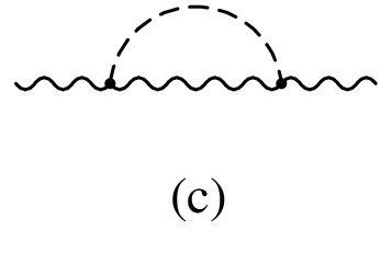
For a presentation of the Lagrangian of the mHDSM in the physical basis of the scalars we refer the reader to [11]. We remark that the matrices ${\cal T}$ and ${\cal R}$ can be eliminated from the Lagrangian by making use of the unitarity of $\tilde{\cal U}$ and the orthogonality of $\tilde{\cal V}$, respectively, in equation (24). The Feynman diagrams which contribute to the vacuum polarizations in the mHDSM are depicted in figure 1.³³ 3 There are also tadpole diagrams, but they are irrelevant for the computation of the oblique parameters.

Diagrams of type (a) are independent of $q^{2}$. Therefore they affect only $T$. It is also necessary to compute type (a) diagrams if we want to demonstrate equation (11) in the mHDSM, which we did; except for this purpose, type (a) Feynman diagrams are irrelevant in the computation of $S$, $U$, $V$, $W$, and $X$, and will henceforth not be considered in this paper.

There are no type (c) diagrams for vacuum polarizations involving either one or two photons—see the mHDSM Lagrangian in [11]. The type (c) diagrams are only relevant for $A_{WW}$ and $A_{ZZ}$.

In the mHDSM all the oblique parameters, except $T$, are ultraviolet-finite after summation over all the Feynman diagrams but before subtraction of the SM expression. The parameter $T$, on the other hand, only becomes non-divergent after the subtraction of the SM Higgs-boson loops, as shown in [11].

We begin by quoting the result for $T$ from [11]:

where $m_{a}$ denotes the mass of the charged scalars $S_{a}^{\pm}$ and $\mu_{b}$ denotes the mass of the neutral scalar $S_{b}^{0}$. The second term in the right-hand side (RHS) of equation (28) contains a sum over all pairs of different physical neutral scalars, i.e. $2\leq b<b^{\prime}\leq m$; similarly, the third term in that RHS contains a sum over all pairs of different physical charged scalars, i.e. $2\leq a<a^{\prime}\leq n$. The last term in the RHS of equation (28) consists of the subtraction, from the rest of $\bar{T}$, of the SM result. In that subtraction, $m_{h}$ is the mass of the sole physical neutral scalar of the SM, the Higgs particle. The well-known [14] function $F$ is given by

We depict this function in figure 2.

Next we write down the results for $\bar{S}$, $\bar{U}$, and $\bar{X}$:

An explicit SM subtraction occurs in both $\bar{S}$ and $\bar{U}$. In $\bar{X}$, on the other hand, such an explicit SM subtraction, showing the mass $m_{h}$ of the SM Higgs boson, does not occur, because $\bar{X}$ relates to $A_{\gamma Z}\left(q^{2}\right)$, and neutral particles—like the SM Higgs boson—do not couple to the photon. Still, the SM subtraction has been performed in $\bar{X}$, as elsewhere, in order to remove, from the sum over the charged scalars $S_{a}^{\pm}$, the Goldstone-boson ($a=1$) term. The explicit forms of the two functions $G\left(I,J,Q\right)$ and $\hat{G}\left(I,Q\right)$ are found in equations (C2) and (C5) of appendix C. Notice that, contrary to what happens to the function $F\left(I,J\right)$ in equation (29), the function $G\left(I,J,Q\right)$ does not vanish when its first two arguments $I$ and $J$, i.e. the squared masses of the two scalar particles in the loop of a type (b) diagram, are equal. In $\bar{S}$, the terms

are meaningful since

as can be verified by using equations (A5), (A6), (A8), and (A9); therefore, the terms (33) are invariant under a scaling of all the scalar masses by a common factor.

In order to write down formulae for $\bar{V}$ and $\bar{W}$ we need the functions $H\left(I,J,Q\right)$ and $\hat{H}\left(I,Q\right)$ in equations (C7) and (C10) of appendix C. We have

Scalar $SU(2)$ singlets with electric charge $Q\neq 0,\pm 1$ cannot mix with the scalars discussed in the previous two sections. Moreover, they couple to the photon and $Z^{0}$ but do not couple to the $W^{\pm}$. Also, there are no off-diagonal couplings among different scalars with the same charge $Q$—for the Lagrangian, see [11]. Therefore, without loss of generality, we may confine ourselves to a single scalar $SU(2)$ singlet, with mass $m$ and electric charge $Q$. In [11] we have shown that, for such a scalar,

Since it does not couple to the $W^{\pm}$ gauge bosons, $A_{WW}=0$ and therefore

too.

The fact that there are no type (c) diagrams, and that two identical scalars occur in the loop of type (b) diagrams, greatly facilitates the computation of the other oblique parameters. The results are

and the remaining oblique parameters are proportional to $\bar{S}$:

In this paper we have calculated the oblique parameters—defined in a fashion appropriate for new physics at a scale not necessarily much higher than the Fermi scale [1]—in the standard $SU(2)\times U(1)$ electroweak gauge theory supplemented by an arbitrary number of scalar $SU(2)$ doublets with hypercharge $1/2$ and scalar $SU(2)$ singlets with arbitrary hypercharges.

We have found that the oblique parameters may be written in terms of only two mixing matrices ${\cal U}$ and ${\cal V}$, which parametrize the mixing of the charge-1 and charge-0 scalars, respectively. These matrices take care simultaneously of the mixing of $SU(2)$-doublet scalars and $SU(2)$-singlet scalars, because ${\cal U}$ is part of a larger unitary matrix $\tilde{\cal U}$, while $\mbox{Re}\,{\cal V}$ and $\mbox{Im}\,{\cal V}$ are parts of a larger real orthogonal matrix $\tilde{\cal V}$. The expressions for the oblique parameters require only five functions $F\left(I,J\right)\left/m_{W}^{2}\right.$, $G\left(I,J,Q\right)$, $\hat{G}\left(I,Q\right)$, $H\left(I,J,Q\right)$, and $\hat{H}\left(I,Q\right)$, of the squared scalar masses $I$ and $J$ and of the squared gauge-boson masses $Q=m_{W}^{2}$ or $Q=m_{Z}^{2}$. We have depicted those functions in figures 2–5.

We note that for a model which has a compact spectrum, in the sense that all the scalar masses—except for the mass of the Higgs particle—are close together, while they are all large compared to $m_{Z}$, all those functions are usually smaller than $F\left(I,J\right)\left/m_{W}^{2}\right.$, which grows like [15] $\left(\!\sqrt{I}-\sqrt{J}\right)^{2}$ and only appears in the parameter $T$. This is one reason why in general we expect $T$ to be dominant in the oblique corrections.⁴⁴ 4 One exception is the effective charge in atomic parity violation, in which $T$ is multiplied by a very small factor and $S$ may dominate [1]. Another exception is the case where only scalar singlets with electric charges other than $0,\pm 1$ are present, because then $T=0$ [11]. The other reason for the dominance of $T$ is the relatively large factor $\left.g^{2}\right/\left(64\pi^{2}\alpha\right)=\left.1\right/\left(16\pi s_{W}^{2}\right)$ contained in $T$—see equations (8) and (28)—which multiplies $F\left(I,J\right)\left/m_{W}^{2}\right.$; the oblique parameters other than $T$ have smaller factors.

The functions $H\left(I,J,Q\right)$ and $\hat{H}\left(I,Q\right)$ tend to zero when $I/Q$ and $J/Q$ grow. The function $\hat{G}\left(I,Q\right)$ grows like $\ln{\left(I/Q\right)}$; pure logarithms of the masses of the scalars also appear in the expression for $S$, and they may render that parameter relatively large even if the masses of the new scalars are all equal. The function $G\left(I,J,Q\right)$ is small for $I=J$ but it becomes sizable whenever $I$ and $J$ are quite far apart, even if they are both much larger than $Q$, i.e. than the electroweak scale.

References

• [1] I. Maksymyk, C.P. Burgess, and D. London, Beyond S, T, and U, Phys. Rev. D 50 (1994) 529 [hep-ph/9306267].
• [2] B.W. Lynn, M.E. Peskin, and R.G. Stuart, in Physics at LEP, J. Ellis and R.D. Peccei eds. (CERN, Geneva, 1986);
D.C. Kennedy and B.W. Lynn, Electroweak radiative corrections with an effective Lagrangian: Four-fermion processes, Nucl. Phys. B 322 (1989) 1.
• [3] M.E. Peskin and T. Takeuchi, A new constraint on a strongly interacting Higgs sector, Phys. Rev. Lett. 65 (1990) 964;
G. Altarelli and R. Barbieri, Vacuum-polarization effects of new physics on electroweak processes, Phys. Lett. B 253 (1991) 161;
M.E. Peskin and T. Takeuchi, Estimation of oblique electroweak corrections, Phys. Rev. D 46 (1992) 381.
G. Altarelli, R. Barbieri, and S. Jadach, Toward a model-independent analysis of electroweak data, Nucl. Phys. B 369 (1992) 3 [erratum ibid. B 376 (1992) 444].
• [4] G.C. Branco, L. Lavoura, and J.P. Silva, CP violation (Oxford University Press, New York, 1999), chapter 11.
• [5] W.M. Yao et al. (Particle Data Group), Review of particle physics, J. Phys. G (Particles and Fields) 33 (2006) 1.
• [6] J. Erler and P. Langacker in [5], p. 119.
• [7] A. Sirlin, Radiative corrections in the S​U​(2)L×U⁡(1)SU(2)_{L}\times U(1) theory: A simple renormalization framework, Phys. Rev. D 22 (1980) 971.
• [8] W. Hollik, Radiative corrections in the Standard Model and their role for precision tests of the electroweak theory, Fortschr. Phys. 38 (1990) 165.
• [9] M. Böhm, A. Denner, and H. Joos, Gauge theories of strong and electroweak interaction, B.G. Teubner, Stuttgart/Leipzig/Wiesbaden (2001), chapter 4.6.
• [10] For references see [5], p. 526.
• [11] W. Grimus, L. Lavoura, O.M. Ogreid, and P. Osland, A precision constraint on multi-Higgs-doublet models, arXiv:0711.4022 [hep-ph].
• [12] W. Grimus and H. Neufeld, Radiative neutrino masses in an S​U​(2)×U⁡(1)SU(2)\times U(1) model, Nucl. Phys. B 325 (1989) 18.
• [13] W. Grimus and L. Lavoura, Soft lepton-flavor violation in a multi-Higgs-doublet seesaw model, Phys. Rev. D 66 (2002) 014016 [hep-ph/0204070].
• [14] M.J.G. Veltman, Limit on mass differences in the Weinberg model, Nucl. Phys. B 123 (1977) 89.
• [15] R. Barbieri, L.J. Hall, and V.S. Rychkov, Improved naturalness with a heavy Higgs: An alternative road to LHC physics, Phys. Rev. D 74 (2006) 015007 [hep-ph/0603188].