Call admission control algorithm for pre-stored VBR video streams
Abstract
We examine the problem of accepting a new request for a pre-stored VBR video stream that has been smoothed using any of the smoothing algorithms found in the literature. The output of these algorithms is a piecewise constant-rate schedule for a Variable Bit-Rate (VBR) stream. The schedule guarantees that the decoder buffer does not overflow or underflow. The problem addressed in this paper is the determination of the minimal time displacement of each new requested VBR stream so that it can be accomodated by the network and/or the video server without overbooking the committed traffic. We prove that this call-admission control problem for multiple requested VBR streams is NP-complete and inapproximable within a constant factor, by reducing it from the Vertex Color problem. We also present a deterministic morphology-sensitive algorithm that calculates the minimal time displacement of a VBR stream request. The complexity of the proposed algorithm make it suitable for real-time determination of the time displacement parameter during the call admission phase.
Keywords:
Variable Bit-Rate Stream, Call-Admission Control, Time Displacement, 3SUM hard, constant factor inapproximable1 Introduction
A significant portion of the forecasted network traffic is expected to be multimedia (e.g. voice and video) traffic. New services such as video-on-demand (VoD) and TV broadcasting are currently under massive deployment. One of the salient characteristics of video traffic is that it usually exhibits high variability in its bandwidth demands in different time scales. The need to better understand the bandwidth demands of video streams is essential for proper resource provisioning of both the network resources and the resources of the video servers when stored video is transported. Proper resource dimensioning has direct correlation with the quality of the recovered video on the decoder and, therefore, a variety of techniques have been proposed in the past.
Significant work has been done in the literature in the area of statistical modeling of video traffic for resource provisioning purposes, so that it can be effectively transported over packet-switched networks [2, 3, 4, 9, 11]. In most cases, the objective of these efforts is to build a general model that can be used for resource dimensioning for all the video traffic transported over the network. In some cases, the long-range dependence (LRD) characteristic of video traffic is exploited to create a model of the traffic source [2, 8, 12]. These methods, in general, characterize the traffic source based on its statistical properties, and provide value when the video stream is not known a-priori. However, when dealing with pre-stored video, the resource dimensioning process can be made deterministic and any statistical technique is of limited value since it does not capture the exact dynamics of the video stream in the time domain.
In video applications that transport stored video over a packet-switched network, the resource provisioning process can take advantage of the fact that video streams can be pre-processed offline. During the pre-processing of a video stream, a transmission schedule is typically computed to minimize its rate variability and, therefore, facilitate the resource provisioning and the call admission control process. The reduction in rate variability is done by work-ahead smoothing, i.e. sending more data to the receiver with respect to its playback time. Significant work can be found in the literature in the area of work-ahead video smoothing [6, 10, 13, 15]. The general idea behind most of these algorithms is to maximize the time intervals (rate segments) at which a transmission rate for the video stream is used without causing under/overflow of the receiver buffer. The algorithms differ in the selection of the starting point of these rate segments. The output of these algorithms is a piecewise constant-rate schedule for the smoothed video stream. The schedule guarantees that the decoder buffer does not overflow or underflow. Due to the fact that computing the smoothing schedule is not a trivial process and cannot be performed online, the pre-computed smoothed schedules of a video file for various decoder profiles can be stored along with the file itself in the video servers, so that they can be used at the time of the corresponding video request to guarantee a deterministic quality at the decoder.
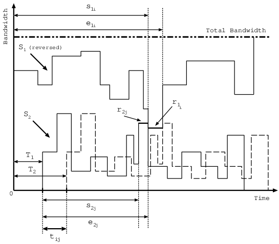
The problem addressed by this paper is that of accepting a new request for a pre-stored VBR video stream that has been pre-smoothed using any of the smoothing algorithms. Since the request can come at any particular point in time, the problem is related to the accomodation of the new request provided that the envelope of the dynamics of the committed traffic, and therefore, the envelope of the available bandwidth in the channel, does not introduce overallocation at any time interval (see Fig. 1). The goal is to displace the pre-computed smoothed schedule of the new request into the future to avoid overallocation. More specifically, we want to find the minimum time displacement of the new schedule so that the channel can accomodate the new request. The problem described is an optimization problem that can be extended in several ways. For example, given a set of requests, find the displacement points of the associated schedules so that the overall schedule is the smoothest.
In this paper we present two algorithms that solve the problem of computing the minimum dispacement of a new request, also referred as the two Stream Scheduling problem (2-SS): (i) a simple algorithm with complexity, and (ii) a morphology-sensitive algorithm with lower computational complexity. The morphology-sensitive algorithm makes specific observations about the smoothed schedule so that certain peaks can be skipped by the algorithm to speed-up the final calculation considerably, depending on the input. Then we present a lower bound on the complexity of the 2-SS problem, which is shown to belong in the 3SUM-hard problem group. We also demonstrate that the problem of computing the minimum displacement of multiple new requests (also referred to as the Multiple Stream Scheduling problem or m-SS) is NP-complete, and cannot be polynomially approximated within a constant factor. This is proven by reducing the String Pack problem to m-SS. String Pack was introduced and shown NP-complete in [14]. To obtain the approximability results, we further reduce Vertex Color[16] to String Pack. This reduction yields new hardness of approximability bounds for String Pack, thus improving previous results.
The rest of this paper is organized as follows: In Section 2, we present the formal definition of the problem for call admission of two VBR streams (or equivalently the admission control of a new request over the envelope of available bandwidth in a channel). We also propose two algorithms that are efficient for the 2-SS problem. In Section 3, we extend the problem to multiple streams. We prove that the problem of admitting multiple streams is NP-complete by reducing the String Pack problem to it. Finally, in Section 4 we conclude the paper with a summary of this work.
2 Admission Control of a new request
2.1 Formal definition
The input of the Two Stream Scheduling (2-SS) problem is two ortholinear traffic envelopes (streams) and of total length and respectively and the channel bandwidth . A stream envelope can be described by an ordered set of triplets , with being the height value (bandwidth demand of video) and and the starting and ending time points of the th peak respectively, of a total of non-overlapping peaks in the stream. Let be the length of the th peak. For the 2-SS problem, consists of such triplets and of triplets.

We consider being requested and transmitted at time point , so being fixed at that position. This allows us to subtract its content allocation from the total bandwidth, creating a reverse envelope, as in Fig. 1. Basically, stream corresponds to the committed traffic. The second stream can be displaced by a positive time interval to its right, resulting in delayed transmission. We assume that the envelopes are rigid and none of the peaks can be altered either in length or height. The order of the peaks is fixed.
Let be displaced by time units. An intersection (time overlap) of the peak triplet from with the peak triplet from occurs when and . The set of all time points such that intersects defines a time interval (referred to from now on as intersection interval) of length , starting at time point and ending at . Intersection parameters are depicted graphically in Fig. 2. The second stream cannot be displaced by any value corresponding to this intersection interval, or there will occur a bandwidth overallocation.
The output of the 2-SS algorithm will be the minimum displacement of , such that there is no bandwidth overallocation. The second stream can be shifted only by a displacement that does not fall into any intersection interval , for and . So, the output of the algorithm could be described as the minimum displacement that does not fall into an intersection interval.
2.2 A morphology sensitive algorithm
In this section we describe an algorithm to solve the 2-SS overallocation problem. The algorithm processes all segments, in order to calculate their intersection interval. It could be the case though that many peaks will not be as high as to intersect. By sorting the peaks by height (bandwidth demand), one can actually calculate the intersection intervals only for the ones that actually intersect and not consider the rest.
Let be the number of peak pairs, where the first peak is selected from envelope and the second from envelope , that have sum of heights greater than the bandwidth and thus define an intersection interval. The algorithm then goes as follows:
- 1.
Sort the peak information (triplets) of both envelopes according to height.
- 2.
Iterate through sorted peaks in and calculate their intersection interval with all peaks from the sorted list of that cause bandwidth overallocation. Stop when the height of the next peak in does not intersect the highest peak of .
- 3.
Sort all intervals according to their starting point.
- 4.
Iterate through sorted intervals, merging them into an aggregate interval, until an interval that does not intersect the aggregate interval is discovered, or we run out of intervals.
- 5.
Output the end point of the aggregate interval as the solution.
For the correctness of the algorithm we can argue that by iterating through all intersecting peaks of both streams, we have discovered all possible time intervals where the second stream cannot be shifted. The first “gap” between the aggregate interval and the currently examined interval will provide the minimum displacement, since any position in the aggregate interval defines a forbidden displacement, belonging to some previously examined intersection interval. The start of the “gap” described above cannot belong to any interval, since, if such an interval existed, its start would occur before the end of the aggregate interval and, as such, before the currently examined interval, which means it would have already been included in the aggregate interval. A visual representation of the procedure can be seen in Fig. 3.

Sorting the peaks by height takes time, the iteration through sorted peaks takes time and sorting all intersection intervals takes time. The merging iteration takes at most time. So the total complexity is .
It should be noted that in the worst case senario where the number of intersecting peaks between the two streams is , the assymptotic complexity becomes , dominated by sorting the intersection intervals’ starting points. We can further improve the running time of this algorithm by excluding intersection interval calculation for peak pairs that result in negative second stream displacement, although such an optimization does not result in any assymptotic gain.
2.3 2-SS scheduling is 3SUM hard
In this section we will prove that 2-SS is 3SUM-hard, a class of problems introduced in [7]. The 3SUM problem is to decide whether there exist integers in a set of integers, such that , which is currently considered to have complexity .
The notion of 3SUM-hardness (or -hardness) is formally introduced in [1, 7], the notation of which we follow. In brief, we will mention that a problem is considered 3SUM-hard if any instance of the 3SUM problem can be reduced to some instance (with a comparable size) of the other problem in time, where is the size of the input.
For our proof, we will need the following definition:
Definition 1
Given two problems and we say that is f(n)-solvable using if every instance of of size can be solved by using a constant number of instances of (of size ) and additional time. We denote this by
To prove that 2-SS is 3SUM-hard, it will be sufficient to show that another 3SUM-hard problem is -solvable using 2-SS. For that purpose, we will use the following 3SUM-hard problem:
Problem: (Segments Containing Points): Given a set of real numbers and a set of pairwise-disjoint intervals of real numbers, is there a real number translation such that ? here indicates the set of intervals in translated by .
was shown 3SUM-hard in [1]. We will now prove the following:
Theorem 2.1
Proof
Given an instance of the problem, we construct two streams in the following way: The intervals in set and real numbers in set are sorted and Stream is constructed to have peaks of height on these intervals and peaks of height in between. The length of is determined by the start of the first interval and end of the last interval in the sorted list and starts at time point 0, with every segment displaced in time by subtracting from each of its coordinates. Stream is constructed with peaks of length with of height 1 at locations defined by the sorted numbers of set , with peaks of height in the intervals in between. The length of is again determined from the smallest and largest elements of ( and respectively) and original displacement of is achieved by subtracting from all peak segment coordinates. We set the channel bandwidth . The construct can be seen in Fig. 4.

We will now argue that the instance of has a solution if and only if the corresponding instance of 2-SS has a displacement solution less than (if there is no solution). From the construction it is obvious that a peak of of height can fit under a height peak of stream only if the corresponding number in falls in the corresponding interval of . If for a certain displacement of we have and there is no overallocation of bandwidth, then all peaks of of height fit under -height peaks of stream , which would imply that . Also, by the same arguments, if there , then displaced by will result in scheduling the two streams with no overallocation.
Based on this result, we can conclude that our morphology-sensitive algorithm for scheduling two streams is within a log factor from optimality.
3 Scheduling multiple streams
We now extend the 2-SS problem to Multiple Stream Scheduling (m-SS), where the input would consist of multiple VBR streams that we want to schedule for transmission over a fixed bandwidth channel. Although we could set different objectives for optimization, we will select minimizing the displacement of the last stream being transmitted. For streams of the same size this is equivalent with minimizing the total length of trasmission, starting from the time point of the first stream transmission and ending when the last stream has been transferred over the channel.
3.1 Multi-stream scheduling is NP-complete
To demonstrate m-SS is NP-complete, we will reduce the String Pack problem to it. The String Pack problem appeared in [14] and was proved hard by reduction from 3-Partition.
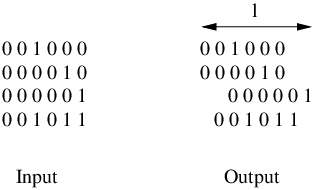
The String Pack is defined as follows: Given a set of strings of length , over the binary alphabet , find a minimum length packing (alignment) of the strings, such that no column has more than one ‘1’. An example of the input and the output of the problem are shown in Fig. 5.
The reduction is straightforward. We will transform the input binary strings into streams with peaks of height for each ’1’ encountered in the string and peaks of height for each ’0’ appearing in the string, as shown in Fig. 6

We let the total available bandwidth , such that no peaks from any stream can overlap. This adheres to the requirement of the String Pack problem not having any column with more than one ’1’. Since the input to the String Pack problem is a set of strings with equal length , minimizing the total length of the outputed alignment is equivalent to minimizing the displacement of the last string. Thus, the output of the m-SS on the transformed strings provides that exact minimum. So we have the following:
Theorem 3.1
String Pack 2-SS
Proof
Given an instance of String Pack, create a 2-SS instance by transforming the binary strings to equivalent streams as described above. The minimum displacement of the last stream to be transmitted, added to the length of the strings, provides the minimum length of the strings’ packing.
The result that m-SS is NP-complete follows from the observation that given a string packing, it can be verified in time (thus polynomial in the input length) that it constitutes a valid solution, where no column in the packing has more than one ’1’, and that the length of the packing is less than a specified length , which would be an input of the decision version of the problem.
3.2 Multiple Stream Scheduling is polynomially inapproximable within a constant
Vertex Color is a well known problem[16], defined as follows: Given a graph , color the vertices of with the minimum number of colors such that for each edge , vertices and have different colors.
It has been shown that Vertex Color is inapproximable within for any , unless [5]. By reducing Vertex Color to String Pack and with the reduction of the latter to m-SS, shown in the previous section, we will demonstrate that any constant approximation of m-SS is NP-hard.
3.2.1 Vertex Color
We now show that VERTEX COLOR reduces to STRING PACK; and that this reduction also yields a polynomial approximation reduction.
Consider a graph , and its vertex-edge incidence matrix. As a running example, we will use the graph given in (Fig. 7) whose incidence matrix is shown below.
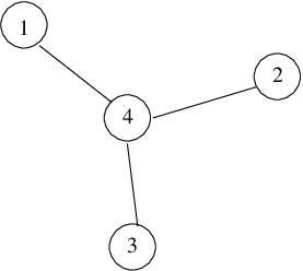
It is clear that the graph can be colored with 2 colors. gets one color, and get another color. Also, the rows of the incidence matrix corresponding to a color group can all be packed with no offset. For example, putting together the rows for gives
But if we try to pack strings from adjacent vertices, we will always get a collision (X); since adjacent vertices have an edge in common. For example
So if we pack rows of the incidence matrix, the vertices the rows correspond to must all be non-adjacent (i.e. can have the same color in a coloring). But if we can color a graph with colors, then we would be able to pack the rows of the incidence matrix into groups. This is a good start, but the String Pack problem has no way of enforcing groups. The strings are allowed to overlap an arbitrary amount. For instance, with the example matrix, it may give the following as a solution:
In order to complete the reduction, we need to flank the incidence matrix with special strings that will force any feasible solution to group the strings in the manner we desire. That is, we want strings to overlap completely, or not at all. That way, if String Pack gives a solution with groups, we know there must exist a coloring of .
It turns out that we can not construct strings that overlap completely, or not at all. We can make strings that overlap completely, or by some small, bounded, amount. This turns out to be sufficient. Consider what overlaps we want to allow and dissallow. In the following, an ’x’ represents a region of the flanking region, and the 0,1 are the rows of our incidence matrix. The following 2 types of alignments should be allowed by the flanking regions.
Complete overlap of incidence matrix rows.
Zero overlap of incidence matrix rows.
But we do not want to allow these following types of alignments, as they interfere with our ’grouping’ of the incidence matrix rows.
Interference of flanking region with incidence matrix rows.
Partial overlap of incidence matrix rows.
The solution to our example would then look like
And we could recover the number of colors from the number of groups is the string alignment (the number of groups is recovered from the span of the solution). Because these flanking strings force grouping, we call them self-aligning strings. Now we procede to describe what these flanking regions (self-aligning strings) look like. To motivate the process, we present an example. In the following set of strings, it is obvious that the first string can not be shifted by any amount to the right and not cause any collisions. The first four characters will always collide with the other strings.
Thus, a first attempt at the self-aligning strings would be consecutive 1’s followed by repeated identity matrices.
The strings are grouped for clarity. In the first 4 blocks, each row gets a sequence of 4 consecutive 1’s. The rest of the blocks are identity matrices. In the region with indentity matrix, any submatrix of 4 consecutive columns is a permutation matrix (ie each row has a 1 in it). Thus, once the 4-consecutive 1’s are shifted into this region, they will always collide with every string.
However, we see these are not self-aligning strings, since the consecutive 1 blocks must be shifted by as much as places before they are in the indentity matrix region of the other strings. For example
To prevent shifts of to we can add the following types of strings to the end of the above strings.
This matrix prevents the first row from shifting an amount to with the second row. We concatenate strings like these for every pair of rows (). The final idea in this construction is that there is no limit on the number of identity matrices we included. Thus we can make these strings as long as we need, until the allowed overlap is a small enough fraction (for example, add identity matrices). For a more precise explanation of self-aligning strings, consult the Appendix.
Theorem 3.2
Vertex Color String Pack
Proof
Given an instance of Vertex Color, create a String Pack instance with the vertex-edge incidence matrix flanked by self-aligning strings. The number of groups in the solution to String Pack is the number of colors in an optimal coloring.
Theorem 3.3
String Pack is hard to approximate (No constant factor approximation).
Proof
We can approximate Vertex Color with String Pack. The approximation depends on the length of the flanking regions. In the next section, we construct flanking strings of size . Thus the total size of the String Pack instance is . Since is the number of vertices, the size of Vertex Color problems are . So if we have an approximation to String Pack, we get an approximation to Vertex Color.
Since Vertex Color is not constant factor approximable, String Pack is not.
4 Conclusions
In this paper, we examined the problem of accepting new video requests for pre-stored VBR video streams that have been pre-smoothed using any of the smoothing algorithms found in the literature. We proved that this problem is an NP-complete problem by reducing it to the String Pack problem.
We also presented two optimization algorithms that can be used to compute the minimum time displacement of a new request to avoid resource overbooking. The morphology-sensitive algorithm is capable of computing the time displacement in time complexity, where is the number of peak pairs when the first peak is selected from the schedule of the new request, and the second from the current traffic envelope, and corresponds to the number of peaks in the schedule of the new video request.
This work can be extended in several ways. In particular, when the cost to the end-user is a variable that needs to be considered, and the cost is a function of the time displacement, the problem can be transformed into one that finds the minimal displacement at the minimally acceptable cost for the end-user.
Other optimization objectives could be analyzed, when given a set of requests, the requirement is to find the displacement points of the associated schedules that produces smoothest combined schedule.
References
- [1] G. Barequet and S. Har-Peled. Polygon-containment and translational min-Hausdorff-distance between segment sets are 3SUM-hard. Int. J. Comput. Geom., 11:465–474, 2001.
- [2] E. Casilari, A. Reyes Lecuona, A. Díaz Estrella, and F. Sandoval. Classification and comparison of modelling strategies for vbr video traffic. In Proceedings of International Teletraffic Congress (ITC-16) ’99, June 1999.
- [3] K. M. Elsayed and H. G Perros. On the effective bandwidth of arbitrary on/off sources. In Proceedings of the Sixth IFIP WG6.3 Conference on Performance of Computer Networks, pages 257–271, October 1995.
- [4] A. I. Elwalid and D. Mitra. Effective bandwidth of general markovian traffic sources and admission control of high speed networks. In Proceedings of IEEE INFOCOM ’93, volume 1, pages 256–265, March 1993.
- [5] U. Feige and J. Kilian. Zero knowledge and the chromatic number. J. Comput. System Sci., 57:187–199, 1998.
- [6] W. Feng. Buffering Techniques for Delivery of Compressed Video in Video-on-Demand Systems. Kluwer Academic Publishers, 1997.
- [7] A. Gajentaan and M. H. Overmars. On a class of problems in computational geometry. Comput. Geom. Theory Appl., 5:165–185, 1995.
- [8] J. Gao and I. Rubin. Multifractal modeling of counting processes of long-range-dependent network traffic, 2001.
- [9] R. Guerin, H. Ahmadi, and M. Naghshineh. Equivalent capacity and its application to bandwidth allocation in high-speed networks. IEEE Journal on Selected Areas in Communications, 9(7):968–981, September 1991.
- [10] Z. Jiang and L. Kleinrock. A general optimal smoothing algorithm. In Proceedings of IEEE INFOCOM ’98, volume 1, 1998.
- [11] G. Kesidis. Modeling to obtain the effective bandwidth of a traffic source in an ATM network. In Proceedings of the Second International Workshop on Modeling, Analysis, and Simulation of Computer and Telecommunication Systems (MASCOTS ’94), pages 318–322, Durham, NC, USA, January 1994.
- [12] G.L. Li and V.O.K. Li. Analysis of transient loss performance impact of long-range-dependence in network traffic. Self-Similar Traffic and Performance Evaluation, 2000.
- [13] J. M. McManus and K. W. Ross. Video-on-demand over ATM: Constant-rate transmission and transport. IEEE Journal on Selected Areas in Communications, 14:1087–1098, August 1996.
- [14] J. Nickerson and S. Skiena. Attention and Communication: Decision Scenarios for Teleoperating Robots. IEEE. Proceedings of the Hawaii International Conference on System Sciences, January 3-6, 2005.
- [15] J. D. Salehi, Z. L. Zhang, J. F. Kurose, and D. Towsley. Supporting stored video: Reducing rate variability and end-to-end resource requirements through optimal smoothing. In Proceedings of ACM SIGMETRICS ’96, volume 1, 1996.
- [16] S.S. Skiena. The Algorithm Design Manual. Springer, 1998.
APPENDIX
Self-Aligning Strings
We now give a more precise account of Self-Aligning strings.
We call a set of strings -aligning if the following properties hold.
- 1.
- 2.
- 3.
is feasible
- 4.
is not feasible for

For a given , there may or may not exists a set of self-aligning strings. We want to show a set exists that will make the reduction in the previous section work. That is, we need to be able to construct them in polynomial time (it is clear from construction that it takes time to construct), and also we need certain constraints on , , and . The following two constraints are sufficient:

First, we want the ‘grouping’ effect. Thus our String-Pack strings should only be able to overlap by at most (or equivalently only allow shifts of at least ) . Since our String-Pack strings contain self-aligning strings as sub-strings; it is obvious that shifts of to are not allowed. Also, once we shift by , the prefix flanker of the shifted string overlaps the suffix flanker of the other string. Thus shifts of to are not allowed (Figure A-2). To make these 2 ranges overlap, we need
The second constraint is to be able to recover the number of groups from the span of the solution. Since two strings will overlap completely only if their corresponding vertices are non-adjacent, we can recover a coloring by grouping strings that overlap completely. Say the answer to String-Pack has groups of strings that overlap completely. Since (from above) each can overlap at most , this means the span of the solution is in the range
If the answer had groups, the range would be
To be able to distinguish the number of completely overlapping groups from the span, we would need
That is, the smallest span from groups is larger than the largest span from groups. This yields
Since , this inequality is achieved if
These constraints are easy to achieve with the outlined construction. To be precise, our self-aligning strings are the rows of
Where is the x matrix
and is the x matrix
The give each row consecutive . Once a string is shifted right by , its will all lie in the region of the other strings (That is, it will have consecutive 1’s overlapping the matrices). Since in this region, a string has a every positions, this shift is not feasible (the s in the shifted string must conflict with a in the other strings). Thus shifts of through are not feasible ( ensures that an is completely in the regios; ensures an isnt shifted past the region). The eliminate shifts of through . This is done explicitly, as can be seen in the construction of the
Thus shifts of through are not feasible. So the maximum overlap, , is bounded by
This is a good result since is fixed for any size . All we want is , which we get for large enough by setting which gets ; a polynomial length string, as desired.