Resummations in QCD hard-scattering
at large and small $x$

The resummation of threshold logarithms is performed in moment space. By taking moments, divergent distributions in $1-z$ (or $s_{4}$) produce powers of $\ln N$, with $N$ the moment variable:

$$\int_{0}^{1}dz\;z^{N-1}\left[{\ln^{m}(1-z)\over 1-z}\right]_{+}={(-1)^{m+1}\over m+1}\ln^{m+1}N+{\cal O}\left(\ln^{m-1}N\right)\,.$$

(7)

If we define moments of the partonic cross section by ${\hat{\sigma}}(N)=\int dz\,z^{N-1}{\hat{\sigma}}(z)$ (PIM) or by ${\hat{\sigma}}(N)=\int(ds_{4}/s)\;e^{-Ns_{4}/s}{\hat{\sigma}}(s_{4})$ (1PI), then the logarithms of $N$ that appear in ${\hat{\sigma}}(N)$ exponentiate.

The resummation follows from the factorization properties of the cross section. We begin the derivation of the resummed cross section by first writing a factorized form for the moment-space infrared-regularized parton-parton scattering cross section, $\sigma_{f_{1}f_{2}\rightarrow F}(N,\epsilon)$, which factorizes as the hadronic cross section

$$\sigma_{f_{1}f_{2}\rightarrow F}(N,\epsilon)={\tilde{\phi}}_{f_{1}/f_{1}}(N,\mu_{F},\epsilon)\;{\tilde{\phi}}_{f_{2}/f_{2}}(N,\mu_{F},\epsilon)\;{\hat{\sigma}}_{f_{1}f_{2}\rightarrow F}(N,\mu_{F},\mu_{R})\,,$$

(8)

with the moments of $\phi$ given by $\tilde{\phi}(N)=\int_{0}^{1}dx\;x^{N-1}\phi(x)$. We factorize the initial-state collinear divergences, regularized by $\epsilon$, into the parton distribution functions, $\phi$, which are expanded to the same order in $\alpha_{s}$ as the partonic cross section, and we thus obtain the perturbative expansion for the infrared-safe partonic short-distance function ${\hat{\sigma}}$.

The partonic short-distance function ${\hat{\sigma}}$ still has sensitivity to soft-gluon dynamics through its $N$ dependence. We then refactorize the moments of the cross section as [4, 8]

	$\displaystyle\sigma_{f_{1}f_{2}\rightarrow F}(N,\epsilon)={\tilde{\psi}}_{f_{1}/f_{1}}\left(N,\mu_{F},\epsilon\right)\;{\tilde{\psi}}_{f_{2}/f_{2}}\left(N,\mu_{F},\epsilon\right)$
	$\displaystyle\hskip-28.45274pt\times\;H_{IL}^{f_{1}f_{2}\rightarrow F}\left(\alpha_{s}(\mu_{R})\right)\;{\tilde{S}}_{LI}^{f_{1}f_{2}\rightarrow F}\left({M\over N\mu_{F}},\alpha_{s}(\mu_{R})\right)\;\prod_{j}{\tilde{J}_{j}}\left(N,\mu_{F},\epsilon\right)+{\cal O}(1/N)\,,$		(9)

where $\psi$ are center-of-mass distributions that absorb the universal collinear singularities from the incoming partons, $H_{IL}$ are $N$-independent hard components which describe the hard-scattering, $S_{LI}$ is a soft gluon function associated with non-collinear soft gluons, and $J$ are functions that absorb the collinear singularities from massless partons, if any, in the final state.

$H$ and $S$ are matrices in color space and we sum over the color indices $I$ and $L$ that describe the color structure of the hard scattering. The hard-scattering function involves contributions from the amplitude of the process and the complex conjugate of the amplitude, $H_{IL}=h_{L}^{*}\,h_{I}$. The soft function $S_{LI}$ represents the coupling of soft gluons to the partons in the scattering. The color tensors of the hard scattering connect together the eikonal lines to which soft gluons couple. One can construct an eikonal operator describing soft-gluon emission and write a dimensionless eikonal cross section, which describes the emission of soft gluons by the eikonal lines [4, 6, 7, 8].

Comparing Eqs. (8) and (9), we see that the moments of the short-distance partonic cross section are given by

	$\displaystyle{\hat{\sigma}}_{f_{1}f_{2}\rightarrow F}(N,\mu_{F},\mu_{R})$	$\displaystyle=$	$\displaystyle{{\tilde{\psi}}_{f_{1}/f_{1}}(N,\mu_{F},\epsilon)\,{\tilde{\psi}}_{f_{2}/f_{2}}(N,\mu_{F},\epsilon)\over{\tilde{\phi}}_{f_{1}/f_{1}}(N,\mu_{F},\epsilon)\,{\tilde{\phi}}_{f_{2}/f_{2}}(N,\mu_{F},\epsilon)}\,H_{IL}^{f_{1}f_{2}\rightarrow F}\left(\alpha_{s}(\mu_{R})\right)$		(10)
			$\displaystyle\times\;{\tilde{S}}_{LI}^{f_{1}f_{2}\rightarrow F}\left(\frac{M}{N\mu_{F}},\alpha_{s}(\mu_{R})\right)\prod_{j}{\tilde{J}_{j}}\left(N,\mu_{F},\epsilon\right)\,.$

All the factors in Eq. (10) are gauge and factorization scale dependent. The constraint that the product of these factors must be independent of the gauge and factorization scale results in the exponentiation of logarithms of $N$ in $\psi/\phi$ and $S_{LI}$ [4, 5].

The soft matrix $S_{LI}$ depends on $N$ through the ratio $M/(N\mu_{F})$, and it requires renormalization as a composite operator. Its $N$-dependence can thus be resummed by renormalization group analysis [17, 18, 19, 20]. However, the product $H_{IL}S_{LI}$ needs no overall renormalization, because the UV divergences of $S_{LI}$ are balanced by those of $H_{IL}$. Thus, we have [4, 8]

	$\displaystyle H^{0}_{IL}$	$\displaystyle=$	$\displaystyle\prod_{i=a,b}Z_{i}^{-1}\;\left(Z_{S}^{-1}\right)_{IC}H_{CD}\left[\left(Z_{S}^{\dagger}\right)^{-1}\right]_{DL}\,,$
	$\displaystyle S^{0}_{LI}$	$\displaystyle=$	$\displaystyle(Z_{S}^{\dagger})_{LB}S_{BA}Z_{S,AI},$		(11)

where $H^{0}$ and $S^{0}$ denote the unrenormalized quantities, $Z_{i}$ is the renormalization constant of the $i$th incoming partonic field, and $Z_{S}$ is a matrix of renormalization constants, which describe the renormalization of the soft function. $Z_{S}$ is defined to include the wave function renormalization necessary for the outgoing eikonal lines that represent any heavy quarks.

From Eq. (11), we see that the soft function $S_{LI}$ satisfies the renormalization group equation [4, 6, 7, 8]

$$\left(\mu{\partial\over\partial\mu}+\beta(g_{s}){\partial\over\partial g_{s}}\right)\,S_{LI}=-(\Gamma^{\dagger}_{S})_{LB}S_{BI}-S_{LA}(\Gamma_{S})_{AI}\,,$$

(12)

where $\beta$ is the QCD beta function and $g_{s}^{2}=4\pi\alpha_{s}$. $\Gamma_{S}$ is an anomalous dimension matrix that is calculated in the eikonal approximation by explicit renormalization of the soft function. In a minimal subtraction renormalization scheme and with $\epsilon=4-n$, where $n$ is the number of space-time dimensions, the soft anomalous dimension matrix is given at one loop by

$$\Gamma_{S}^{(1l)}(g_{s})=-\frac{g_{s}}{2}\frac{\partial}{\partial g_{s}}{\rm Res}_{\epsilon\rightarrow 0}Z_{S}(g_{s},\epsilon)\,.$$

(13)

The process-dependent matrices $\Gamma_{S}$ have been calculated at one loop for all $2\rightarrow 2$ partonic processes; a compilation of results is given in [8]. In processes with trivial or simple color structure $\Gamma_{S}$ is simply a function ($1\times 1$ matrix) while in processes with complex color structure it is a non-trivial matrix in color exchange. For quark-(anti)quark scattering, $\Gamma_{S}$ is a $2\times 2$ matrix [4, 18]; for quark-gluon scattering it is a $3\times 3$ matrix [7]; for gluon-gluon scattering it is an $8\times 8$ matrix [7]. Complete two-loop calculations of soft anomalous dimensions for processes with massless quarks have appeared in [21]. Selected two-loop results for heavy quark production appeared in [22]. We present a sample one-loop calculation in Section 4.1 and a sample two-loop calculation in Section 4.2, both with outgoing massive quarks (see [23]).

The exponentiation of logarithms of $N$ in the ratios $\psi/\phi$ and in the functions $J$ in Eq. (10), together with the solution of the renormalization group equation (12), provide us with the complete expression for the resummed partonic cross section in moment space [4, 6, 7, 8, 24, 25]

	$\displaystyle{\hat{\sigma}}^{res}(N)$	$\displaystyle=$	$\displaystyle\exp\left[\sum_{i}E^{f_{i}}(N_{i})\right]\;\exp\left[\sum_{j}{E^{\prime}}^{f_{j}}(N_{j})\right]$		(14)
			$\displaystyle\hskip-28.45274pt\times\,\exp\left[\sum_{i}2\int_{\mu_{F}}^{\sqrt{s}}\frac{d\mu}{\mu}\;\gamma_{f_{i}/f_{i}}\left(\alpha_{s}(\mu)\right)\right]\;\exp\left[2\,d_{\alpha_{s}}\int_{\mu_{R}}^{\sqrt{s}}\frac{d\mu}{\mu}\;\beta\left(\alpha_{s}(\mu)\right)\right]$
			$\displaystyle\hskip-28.45274pt\times\,{\rm Tr}\left\{H^{f_{1}f_{2}\rightarrow F}\left(\alpha_{s}(\mu_{R})\right)\;\exp\left[\int_{\sqrt{s}}^{{\sqrt{s}}/{\tilde{N}_{j}}}\frac{d\mu}{\mu}\;\Gamma_{S}^{\dagger\,f_{1}f_{2}\rightarrow F}\left(\alpha_{s}(\mu)\right)\right]\right.$
			$\displaystyle\hskip-28.45274pt\left.\times\,{\tilde{S}^{f_{1}f_{2}\rightarrow F}}\left(\alpha_{s}\left(\frac{\sqrt{s}}{\tilde{N}_{j}}\right)\right)\exp\left[\int_{\sqrt{s}}^{{\sqrt{s}}/{\tilde{N}_{j}}}\frac{d\mu}{\mu}\;\Gamma_{S}^{f_{1}f_{2}\rightarrow F}\left(\alpha_{s}(\mu)\right)\right]\right\}\,.$

The sums over $i=1,2$ run over incoming partons. The sum over $j$ is over massless partons, if any, in the final state at lowest order. The resummed expression is valid for either 1PI or PIM kinematics. In 1PI kinematics $N_{i}=N(-t_{i}/M^{2})$, where $t_{i}$ denotes $t$ or $u$, and $N_{j}=N(s/M^{2})$, while in PIM kinematics $N_{i}=N_{j}=N$. Also ${\tilde{N}}=Ne^{\gamma_{E}}$, with $\gamma_{E}$ the Euler constant.

The first exponent in Eq. (14) arises from the exponentiation of logarithms of $N$ in the ratios $\psi/\phi$ of Eq. (10), and is given in the $\overline{\rm MS}$ scheme by

$$E^{f_{i}}(N_{i})=-\int^{1}_{0}dz\frac{z^{N_{i}-1}-1}{1-z}\;\left\{\int^{1}_{(1-z)^{2}}\frac{d\lambda}{\lambda}A_{i}\left(\alpha_{s}(\lambda s)\right)+{\nu}_{i}\left[\alpha_{s}((1-z)^{2}s)\right]\right\}\,,$$

(15)

with $A_{i}(\alpha_{s})=\sum_{n=1}^{\infty}(\alpha_{s}/\pi)^{n}A_{i}^{(n)}$. At one loop, $A_{i}^{(1)}=C_{i}$ which is $C_{F}=(N_{c}^{2}-1)/(2N_{c})$ for a quark or antiquark and $C_{A}=N_{c}$ for a gluon, with $N_{c}$ the number of colors, while $A_{i}^{(2)}=C_{i}K/2$ with $K=C_{A}(67/18-\zeta_{2})-5n_{f}/9$ [26], where $n_{f}$ is the number of quark flavors and $\zeta_{2}=\pi^{2}/6$. Also ${\nu}_{i}=\sum_{n=1}^{\infty}(\alpha_{s}/\pi)^{n}{\nu}_{i}^{(n)}$, with ${\nu}_{i}^{(1)}=C_{i}$.

The second exponent in Eq. (14) arises from the exponentiation of logarithms of $N$ in the functions $J_{j}$ of Eq. (10), and is given by

	$\displaystyle{E^{\prime}}^{f_{j}}(N_{j})$	$\displaystyle=$	$\displaystyle\int^{1}_{0}dz\frac{z^{N_{j}-1}-1}{1-z}\;\left\{\int^{1-z}_{(1-z)^{2}}\frac{d\lambda}{\lambda}A_{j}\left(\alpha_{s}\left(\lambda s\right)\right)-B_{j}\left[\alpha_{s}((1-z)s)\right]\right.$		(16)
			$\displaystyle\hskip 85.35826pt\left.{}-\nu_{j}\left[\alpha_{s}((1-z)^{2}s)\right]\right\}\,.$

Here $B_{j}=\sum_{n=1}^{\infty}(\alpha_{s}/\pi)^{n}B_{j}^{(n)}$ with $B_{j}^{(1)}$ equal to $3C_{F}/4$ for quarks and $\beta_{0}/4$ for gluons, where $\beta_{0}=(11C_{A}-2n_{f})/3$ is the lowest-order $\beta$ function.

The third exponent in Eq. (14) controls the factorization scale dependence of the cross section, and $\gamma_{f_{i}/f_{i}}$ is the moment-space anomalous dimension of the ${\overline{\rm MS}}$ density $\phi_{f_{i}/f_{i}}$. The $\beta$ function in the fourth exponent controls the renormalization scale dependence of the cross section. The constant $d_{\alpha_{s}}$ takes the value $k$ if the Born cross section is of order $\alpha_{s}^{k}$. Explicit expressions for the functions in these four exponents, and related references, are assembled for convenience in Appendix A of Ref. [27].

As noted before, both $H$ and $S$ are process-dependent matrices in color space and thus the trace is taken in Eq. (14). At lowest order, the trace of the product of $H$ and $S$ reproduces the Born cross section. The evolution of the soft function $S$ follows from its renormalization group equation, (12), and is given in terms of the soft anomalous dimension matrix $\Gamma_{S}$.

The exponentials in the resummed partonic cross section can be expanded to any fixed order in $\alpha_{s}$ and then inverted to momentum space to provide explicit results for the higher-order corrections. A fixed-order expansion avoids using a prescription to regulate the infrared singularities in the exponents and thus no prescription is needed to deal with these in this approach (see discussion in Ref. [28]).

We now expand the resummed cross section, Eq. (14), in 1PI kinematics through NNNLO. We provide results here for the case where $\Gamma_{S}$ are trivial (1 $\times$ 1) color matrices. Explicit expressions for the more general case are found through NNLO in [24] and through NNNLO in [25].

At NLO, we find the expression for the soft-gluon corrections

$${\hat{\sigma}}^{(1)}=\sigma^{B}\frac{\alpha_{s}(\mu_{R}^{2})}{\pi}\left\{c_{3}\,{\cal D}_{1}(s_{4})+c_{2}\,{\cal D}_{0}(s_{4})+c_{1}\,\delta(s_{4})\right\}$$

(17)

where $\sigma^{B}$ is the leading-order (LO) term, the LL coefficient is

$$c_{3}=\sum_{i}2\,C_{i}-\sum_{j}C_{j}\,,$$

(18)

with $C_{q}=C_{F}$ and $C_{g}=C_{A}$, and the NLL coefficient $c_{2}$ is defined by $c_{2}=c_{2}^{\mu}+T_{2}$, with

$$c_{2}^{\mu}=-\sum_{i}C_{i}\ln\left(\frac{\mu_{F}^{2}}{M^{2}}\right)$$

(19)

denoting the terms involving logarithms of the factorization scale, and

	$\displaystyle T_{2}$	$\displaystyle=$	$\displaystyle 2{\rm Re}\Gamma_{S}^{(1)}-\sum_{i}\left[C_{i}+2\,C_{i}\,\ln\left(\frac{-t_{i}}{M^{2}}\right)+C_{i}\ln\left(\frac{M^{2}}{s}\right)\right]$		(20)
			$\displaystyle{}-\sum_{j}\left[B_{j}^{(1)}+C_{j}+C_{j}\,\ln\left(\frac{M^{2}}{s}\right)\right]\,$

denoting the scale-independent terms. Again, $t_{i}$ denotes $t$ or $u$, the sums over $i$ run over incoming partons, and the sums over $j$ run over any massless partons in the final state at LO.

We write the NLO $\delta(s_{4})$ terms as $c_{1}=c_{1}^{\mu}+T_{1}$, where

$$c_{1}^{\mu}=\sum_{i}\left[C_{i}\,\ln\left(\frac{-t_{i}}{M^{2}}\right)-\gamma_{i}^{(1)}\right]\ln\left(\frac{\mu_{F}^{2}}{M^{2}}\right)+d_{\alpha_{s}}\frac{\beta_{0}}{4}\ln\left(\frac{\mu_{R}^{2}}{M^{2}}\right)$$

(21)

denotes the terms involving logarithms of the factorization and renormalization scales. Here $\gamma_{q}^{(1)}=3C_{F}/4$ and $\gamma_{g}^{(1)}=\beta_{0}/4$, and $T_{1}$ denotes virtual terms that cannot be derived from the resummation formalism but can be determined by matching to a full NLO calculation for any specified process.

At NNLO, the soft-gluon corrections are

	$\displaystyle{\hat{\sigma}}^{(2)}$	$\displaystyle=$	$\displaystyle\sigma^{B}\frac{\alpha_{s}^{2}(\mu_{R}^{2})}{\pi^{2}}\;\left\{\frac{1}{2}\,c_{3}^{2}\;{\cal D}_{3}(s_{4})+\left[\frac{3}{2}\,c_{3}\,c_{2}-\frac{\beta_{0}}{4}\,c_{3}+\sum_{j}C_{j}\,\frac{\beta_{0}}{8}\right]\;{\cal D}_{2}(s_{4})\right.$		(22)
			$\displaystyle\hskip-42.67912pt\left.{}+\left[c_{3}\,c_{1}+c_{2}^{2}-\zeta_{2}\,c_{3}^{2}-\frac{\beta_{0}}{2}\,T_{2}+\frac{\beta_{0}}{4}\,c_{3}\,\ln\left(\frac{\mu_{R}^{2}}{M^{2}}\right)+c_{3}\,\frac{K}{2}-\sum_{j}\frac{\beta_{0}}{4}\,B_{j}^{(1)}\right]\;{\cal D}_{1}(s_{4})\right\}$
			$\displaystyle{}+\cdots$

where we show explicitly results through next-to-next-to-leading logarithms (NNLL). For a complete expression see [24, 25].

At NNNLO, the soft-gluon corrections are

	$\displaystyle{\hat{\sigma}}^{(3)}$	$\displaystyle=$	$\displaystyle\sigma^{B}\frac{\alpha_{s}^{3}(\mu_{R}^{2})}{\pi^{3}}\;\left\{\frac{1}{8}\,c_{3}^{3}\;{\cal D}_{5}(s_{4})+\left[\frac{5}{8}\,c_{3}^{2}\,c_{2}-\frac{5}{24}\,\beta_{0}\,c_{3}^{2}+\frac{5}{48}\,c_{3}\,\beta_{0}\sum_{j}C_{j}\right]\;{\cal D}_{4}(s_{4})\right.$		(23)
			$\displaystyle\hskip-28.45274pt{}+\left[c_{3}\,c_{2}^{2}+\frac{1}{2}\,c_{3}^{2}\,c_{1}-\zeta_{2}\,c_{3}^{3}+\frac{\beta_{0}^{2}}{12}c_{3}-\frac{\beta_{0}}{3}c_{3}c_{2}-\frac{\beta_{0}}{2}c_{3}T_{2}+\frac{\beta_{0}}{4}c_{3}^{2}\ln\left(\frac{\mu_{R}^{2}}{M^{2}}\right)\right.$
			$\displaystyle\hskip-14.22636pt\left.\left.{}+c_{3}^{2}\frac{K}{2}+c_{2}\frac{\beta_{0}}{6}\sum_{j}C_{j}-c_{3}\sum_{j}\frac{\beta_{0}}{4}B_{j}^{(1)}-\sum_{j}C_{j}\,\frac{3\beta_{0}^{2}}{48}\right]\;{\cal D}_{3}(s_{4})\right\}+\cdots$

where again we show explicitly results through NNLL. The complete expression is given in [25].

In PIM kinematics we simply replace $s_{4}$ by $1-z$, set $s=M^{2}$, and drop the terms with $\ln(-t_{i}/M^{2})$ in the above formulas.

The NNNLO master equation, (23), gives the structure of the soft corrections and can provide the full soft corrections explicitly if all the necessary two-loop and three-loop quantities are known. For processes with non-trivial color structure we are currently limited to NLL or NNLL accuracy. For processes with trivial color structure, such as $b{\bar{b}}\rightarrow H$ [29, 27], all soft-gluon corrections have been determined through NNNLO. Below, the term “N⁽ⁿ⁾LO-N^(l)LL” means that the soft-gluon contributions through N^(l)LL accuracy to the $n$-th order QCD corrections have been included.

The top quark, the heaviest known elementary particle, was discovered in $p{\bar{p}}$ collisions at Run I of the Tevatron in 1995 [30, 31]. More recent measurements at Run II have increased the accuracy of the top mass and cross section measurements (for a review see [32, 33]) and thus require accurate theoretical calculations of top production cross sections and differential distributions. The main partonic channels in $t{\bar{t}}$ production are $q{\bar{q}}\rightarrow t{\bar{t}}$, which is dominant at the Tevatron, and $gg\rightarrow t{\bar{t}}$, which will be dominant at the LHC.

The latest calculation for top-antitop pair hadroproduction includes NNLO soft-gluon corrections to the double differential cross section [34]. Near threshold the soft-gluon corrections dominate the cross section at the Tevatron and contribute sizable enhancements. The form of the corrections and their numerical values depend crucially on the kinematics chosen to describe the process. The NNLO soft corrections were calculated fully to NNLL in both 1PI and PIM kinematics [28, 35]. In addition a good approximation for the next-to-next-to-next-to-leading logarithms (NNNLL) was provided in [34]. The best theoretical result for the cross section is the average of the NNLO-NNNLL cross sections in the two different kinematics [34].

In Fig. 1, we present the NLO and approximate NNLO-NNNLL $t\overline{t}$ cross sections at the Tevatron with $\sqrt{S}=1.96$ TeV using the MRST2002 [36] parton densities. On the left we plot the cross sections as functions of $m_{t}$, the top quark mass, for $\mu=m_{t}$, where $\mu$ denotes the factorization and renormalization scales which we have set equal to each other. On the right we plot the cross sections as functions of $\mu/m_{t}$ with $m_{t}=175$ GeV. The results are given in both 1PI and PIM kinematics together with their average. The NLO cross section depends less on $\mu$ than the LO cross section, as expected. The NNLO-NNNLL cross sections exhibit even less dependence on $\mu$, approaching the scale independence of a true physical cross section. They change by less than 3% in the range $m_{t}/2<\mu<2m_{t}$. For a top mass of 175 GeV the average of the NNLO-NNNLL 1PI and PIM results is $6.77\pm 0.42$ pb, where the uncertainty indicated is from the kinematics. Including all sources of uncertainty (kinematics, scale variation, and uncertainty from the parton distribution functions) we may write the cross section as $6.8\pm 0.6$ pb. This theoretical result is in agreement with the latest experimental result for the cross section at the Tevatron [37, 38]. Finally, we note that NNNLO soft-gluon contributions in the $q{\bar{q}}\rightarrow t{\bar{t}}$ channel were presented in [25]. These NNNLO-NNLL corrections further stabilize the scale dependence of the cross section at the Tevatron.

Single top quark production provides a way to directly measure electroweak properties of the top quark, such as the $V_{tb}$ CKM matrix element. It also allows a deeper study of electroweak theory since the top quark mass is of the same order of magnitude as the electroweak symmetry breaking scale, and may be useful in the discovery of new physics. Therefore it is crucial to have accurate theoretical predictions for the cross section.

The cross section for single top quark production is less than the $t{\bar{t}}$ cross section and the backgrounds to the production processes make the extraction of the single top signal challenging. Intensive searches for single top quark events at the Tevatron have recently produced evidence of such events [39, 40]. The LHC has good potential for observation and further analysis of single top events.

Single top quarks can be produced through three distinct partonic processes. One is $t$-channel production, $qb\rightarrow q^{\prime}t$ and ${\bar{q}}b\rightarrow{\bar{q}}^{\prime}t$, via the exchange of a space-like $W$ boson, a second is $s$-channel production, $q{\bar{q}}^{\prime}\rightarrow{\bar{b}}t$, via the exchange of a time-like $W$ boson, and a third is associated $tW$ production, $bg\rightarrow tW^{-}$.

The threshold corrections to single top production have been calculated for both the Tevatron and LHC colliders through NNNLO [41, 42, 43]. At the Tevatron the $t$-channel process is numerically dominant, but the higher-order corrections are relatively small. The $s$-channel is smaller, but receives large corrections and it was shown that the threshold soft-gluon corrections dominate the cross section. Associated $tW$ production is quite minor, although it also has large $K$ factors, defined as the ratios of the higher-order cross sections to the LO cross section. At the LHC the $t$ channel is again dominant, but the second largest channel is $tW$ production; the $s$ channel is numerically the smallest. Below we provide some numerical results for all three channels at both the Tevatron and the LHC colliders using the MRST2004 parton densities [44]. We add the soft-gluon corrections through NNNLO to the complete NLO cross section [45, 46].

We begin with single top production at the Tevatron [41] with $\sqrt{S}=1.96$ TeV. For $t$-channel production, the NNNLO-NLL cross section is $\sigma^{t-{\rm channel}}(m_{t}=175\,{\rm GeV})=1.08^{+0.02}_{-0.01}\pm 0.06$ pb, where the first uncertainty is from variation of the factorization and renormalization scales, $\mu_{F}$ and $\mu_{R}$, between $m_{t}/2$ and $2m_{t}$, and the second is due to the parton distribution functions. For the $s$ channel, the corresponding cross section is $\sigma^{s-{\rm channel}}(m_{t}=175\,{\rm GeV})=0.49\pm 0.02\pm 0.01$ pb. Finally, in the $tW$ channel $\sigma^{tW}(m_{t}=175\,{\rm GeV})=0.13\pm 0.02\pm 0.02$ pb. We note that the cross sections for antitop production at the Tevatron are identical to those for single top production in each channel.

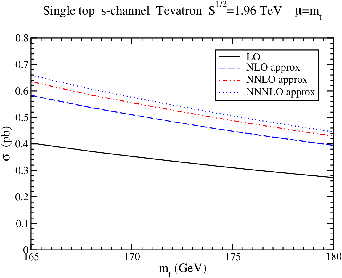
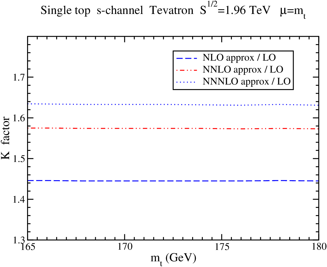
In Fig. 2 we plot the cross section and the $K$ factors for single top quark production at the Tevatron in the $s$ channel setting both the factorization and renormalization scales to $\mu=m_{t}$. We plot the LO cross section and the approximate NLO, NNLO, and NNNLO cross sections at NLL accuracy. The $K$ factors are quite large, thus showing that the corrections provide a big enhancement to the cross section.

We continue with single top production at the LHC [42] with $\sqrt{S}=14$ TeV. For the $t$ channel the threshold corrections are not a good approximation of the complete corrections. The NLO cross section for top production $\sigma^{t-{\rm channel}}_{\rm top}(m_{t}=175\,{\rm GeV})=146\pm 4\pm 3$ pb. For antitop production the corresponding result is $\sigma^{t-{\rm channel}}_{\rm antitop}(m_{t}=175\,{\rm GeV})=89\pm 3\pm 2$ pb. For the $s$ channel, the soft-gluon corrections are relatively large and the soft-gluon approximation is good. The NNNLO-NLL cross section is $\sigma^{s-{\rm channel}}_{\rm top}(m_{t}=175\,{\rm GeV})=7.23^{+0.53}_{-0.45}\pm 0.13$ pb for single top production and $\sigma^{s-{\rm channel}}_{\rm antitop}(m_{t}=175\,{\rm GeV})=4.03^{+0.10}_{-0.12}\pm 0.10$ pb for single antitop production. Finally, for $tW$ production the cross section is $\sigma^{tW}(m_{t}=175\,{\rm GeV})=41.1\pm 4.1\pm 1.0$ pb, which is identical to that for associated antitop production. In Fig. 3 we plot the cross section and $K$ factors for associated $tW$ production at the LHC setting the scales to $\mu=m_{t}$. As seen from the plots, the soft-gluon corrections are large for this process.

$W$-boson production in hadron colliders can be used in testing the Standard Model and in estimating backgrounds to Higgs production and new physics. Precise calculations for $W$ production at large transverse momentum, $Q_{T}$, are needed to identify signals of new physics which may be expected to enhance the $Q_{T}$ distribution at high $Q_{T}$.

Analytical NLO calculations of the cross section for $W$ production at large transverse momentum were presented in Refs. [47, 48], where numerical results were also presented for the Fermilab Tevatron. Numerical NLO results for $W$ production at the LHC were more recently presented in [49]. The NLO corrections enhance the $Q_{T}$ distribution of the $W$ boson and they reduce the factorization and renormalization scale dependence of the cross section.

A recent theoretical study [50] included soft-gluon corrections through NNLO, which provide additional enhancements and a further reduction of the scale dependence. The complete NNLL terms were calculated and an approximation for the NNNLL terms was derived at NNLO. Numerical results with these soft corrections were calculated for $W$ production at the Tevatron [50] and the LHC [49].

Here we discuss $W$ production at large transverse momentum at the LHC with $\sqrt{S}=14$ TeV using the MRST2002 parton densities [36]. The LO partonic processes for the production of a $W$ boson and a parton are $qg\rightarrow Wq$ and $q{\bar{q}}\rightarrow Wg$. The electroweak coupling $\alpha(M_{Z}^{2})$ is evaluated at the mass of the $Z$ boson, and standard values [51] are used for the various electroweak parameters. In the numerical results we present the sum of cross sections for $W^{-}$ and $W^{+}$ production. The $W$ bosons at the LHC will be detected primarily through their leptonic decay products e.g., $W^{-}\rightarrow\ell\bar{\nu}_{\ell}$, therefore the cross sections presented here should be multiplied by the appropriate branching ratios.

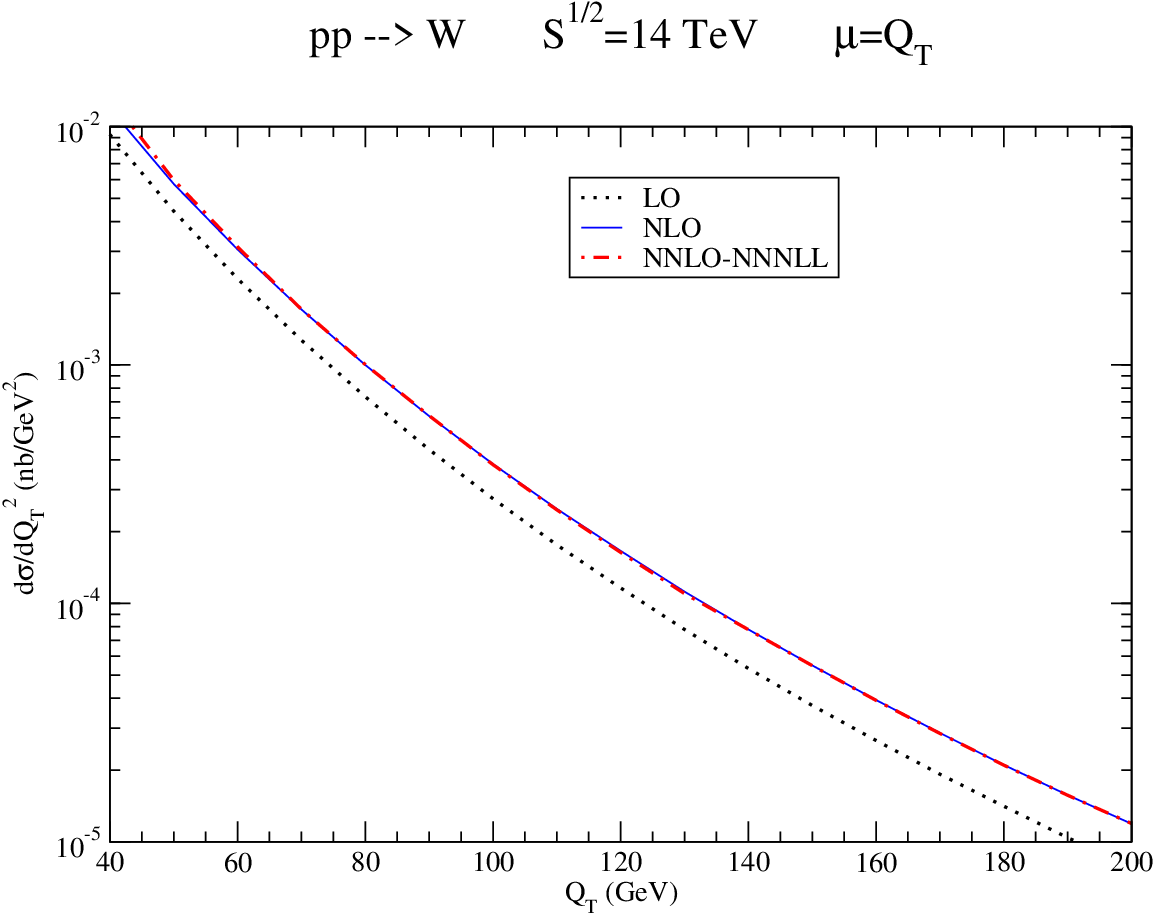
In Fig. 4 (left plot) we plot the transverse momentum distribution, $d\sigma/dQ_{T}^{2}$, at high $Q_{T}$ for $W$ production at the LHC. We set $\mu_{F}=\mu_{R}=Q_{T}$ and denote this common scale by $\mu$. We plot LO, NLO, and NNLO-NNNLL results using the corresponding parton densities. As seen from the plot, the NLO corrections provide a significant enhancement of the LO $Q_{T}$ distribution. The NNLO-NNNLL corrections provide a rather small further enhancement of the $Q_{T}$ distribution. However, the NNLO-NNNLL corrections can be much bigger for other choices of factorization and renormalization scales. The NLO corrections increase the LO result by about 30% to 50% in the $Q_{T}$ range shown. In contrast, the NNLO-NNNLL/NLO ratio for this scale is rather small. Part of the reason for this is that the NNLO parton distribution functions are significantly smaller than the NLO pdf.

On the plot on the right in Fig. 4 we show the scale dependence of $d\sigma/dQ_{T}^{2}$ for $Q_{T}=150$ GeV versus $\mu/Q_{T}$ over two orders of magnitude. It is interesting to note that the scale dependence of the cross section is not reduced when the NLO corrections are included. This is due to the fact that the cross section is dominated by the process $qg\rightarrow Wq$. The gluon density in the proton, at fixed $x$ less than ${\sim}0.01$, increases rapidly with scale. Thus, the $\mu_{R}$ and $\mu_{F}$ dependencies cancel one another to a large extent. However, we have an improvement in the scale variation when the NNLO-NNNLL corrections are added. The NNLO-NNNLL result displays very little scale dependence.

The search for the Higgs boson [52] is one of the most important goals at the Tevatron and the LHC colliders [53]. The main Standard Model production channel at these colliders is $gg\rightarrow H$. However, the channel $b{\bar{b}}\rightarrow H$ can be competitive in the Minimal Supersymmetric Standard Model at high $\tan\beta$, with $\tan\beta$ the ratio of the vacuum expectation values for the two Higgs doublets. The complete NNLO QCD corrections for this process were calculated in [54].

Complete expressions for the soft-gluon corrections at NNNLO were presented in [27, 29]. However, it is known at NNLO that the soft corrections alone are not a good approximation of the full corrections [54, 27]. Purely collinear terms [55, 56, 27] have to be included to provide an accurate calculation. An approximation for the collinear terms through NNLL accuracy at NNNLO was provided in [27].

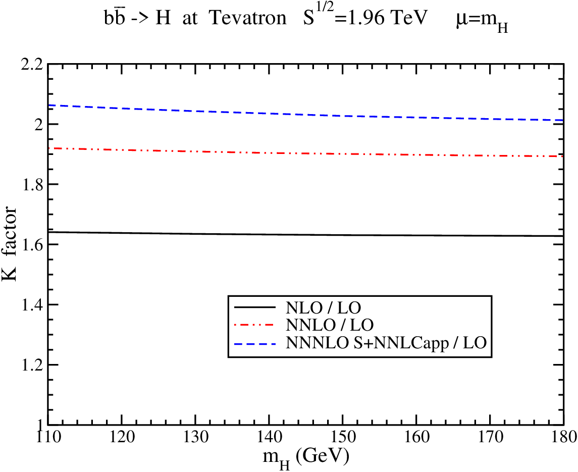
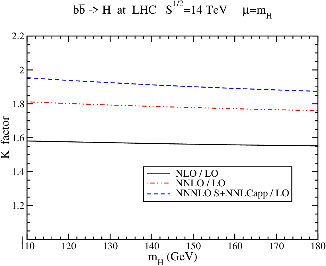
We now present numerical results for $b{\bar{b}}\rightarrow H$ at the Tevatron and the LHC [27] using the MRST2006 parton densities [57]. Figure 5 shows the $K$ factors for Higgs production via $b{\bar{b}}\rightarrow H$ at the Tevatron (left) and the LHC (right), with $\mu=m_{H}$. The complete NLO corrections increase the LO result by around 60% at both the Tevatron and the LHC. Inclusion of the complete NNLO corrections futher increases the cross section: the NNLO $K$ factor is around 1.9 at the Tevatron and 1.8 at the LHC. By including at NNNLO the sum of the complete soft-gluon corrections and the collinear approximate NNLL corrections (S+NNLLapp), we find further enhancement. From the study of the contributions of the soft and collinear terms at NLO and NNLO at both the Tevatron and the LHC we expect that the NNNLO S+NNLCapp curve provides a good approximation of the complete NNNLO cross section. The NNNLO S+NNLCapp $K$ factor is between 2.06 and 2.01 at the Tevatron and between 1.95 and 1.87 at the LHC for Higgs masses ranging between 110 and 180 GeV, which is a significant addition to the NNLO result.

In this subsection we calculate the integral $I_{1l}$ for the one-loop diagram in Fig. (7) with eikonal lines representing outgoing massive quarks. This one-loop integral is given by

$$I_{1l}=g_{s}^{2}\int\frac{d^{n}k}{(2\pi)^{n}}\frac{(-i)g_{\mu\nu}}{k^{2}}\frac{v_{i}^{\mu}}{v_{i}\cdot k}\,\frac{(-v_{j}^{\nu})}{(-v_{j}\cdot k)}\,.$$

(25)

Using Feynman parameterization, this integral can be rewritten as

$$I_{1l}=-2ig_{s}^{2}\,\frac{v_{i}\cdot v_{j}}{(2\pi)^{n}}\int_{0}^{1}dx\int_{0}^{1-x}dy\int\frac{d^{n}k}{\left[xk^{2}+yv_{i}\cdot k+(1-x-y)v_{j}\cdot k\right]^{3}}\,.$$

(26)

After several manipulations, Eq. (26) becomes

	$\displaystyle I_{1l}$	$\displaystyle=$	$\displaystyle\frac{\alpha_{s}}{\pi}\,(-1)^{-1-\epsilon/2}\,2^{5\epsilon/2}\,\pi^{\epsilon/2}\,\Gamma\left(1+\frac{\epsilon}{2}\right)(1+\beta^{2})\int_{0}^{1}dx\,x^{-1+\epsilon}(1-x)^{-1-\epsilon}$
			$\displaystyle\hskip-45.5244pt{}\times\left\{\int_{0}^{1}dz\left[4z\beta^{2}(1-z)+1-\beta^{2}\right]^{-1}-\frac{\epsilon}{2}\int_{0}^{1}dz\frac{\ln\left[4z\beta^{2}(1-z)+1-\beta^{2}\right]}{4z\beta^{2}(1-z)+1-\beta^{2}}+{\cal O}\left(\epsilon^{2}\right)\right\}$

where here $\beta=\sqrt{1-4m^{2}/s}$, with $m$ the quark mass, and we have used the relations $v_{i}\cdot v_{j}=(1+\beta^{2})/2$ and $v_{i}^{2}=v_{j}^{2}=(1-\beta^{2})/2$.

The integral over $x$ in Eq. () contains both ultraviolet (UV) and infrared (IR) singularities. We isolate the UV singularities and find that

$$\int_{0}^{1}dx\,x^{-1+\epsilon}\,(1-x)^{-1-\epsilon}=\frac{1}{\epsilon}+{\rm IR}.$$

(28)

After calculating the integrals over $z$ in Eq. (), we find that the UV poles and constant terms of $I_{1l}$ are

	$\displaystyle I_{1l}^{UV}$	$\displaystyle=$	$\displaystyle\frac{\alpha_{s}}{\pi}\frac{(1+\beta^{2})}{2\beta}\left\{\frac{1}{\epsilon}\ln\left(\frac{1-\beta}{1+\beta}\right)+\frac{1}{2}\left(4\ln 2+\ln\pi-\gamma_{E}-i\pi\right)\ln\left(\frac{1-\beta}{1+\beta}\right)\right.$		(29)
			$\displaystyle\left.{}+\frac{1}{4}\ln^{2}(1+\beta)-\frac{1}{4}\ln^{2}(1-\beta)-\frac{1}{2}{\rm Li}_{2}\left(\frac{1+\beta}{2}\right)+\frac{1}{2}{\rm Li}_{2}\left(\frac{1-\beta}{2}\right)\right\}.$

Complete one-loop calculations for heavy quark production in axial gauge were presented in Ref. [4].

In this subsection we calculate the two-loop integral $I_{2l}$ for the quark-loop diagram in Fig. (8) given by

	$\displaystyle I_{2l}$	$\displaystyle=$	$\displaystyle(-1)n_{f}g_{s}^{4}\int\frac{d^{n}k}{(2\pi)^{n}}\frac{d^{n}l}{(2\pi)^{n}}\frac{v_{i}^{\mu}}{v_{i}\cdot k}\frac{(-v_{j}^{\rho})}{(-v_{j}\cdot k)}\frac{(-i)g_{\mu\nu}}{k^{2}}\frac{(-i)g_{\rho\sigma}}{k^{2}}$		(30)
			$\displaystyle\times{\rm Tr}\left[-i\gamma^{\nu}\frac{il\!\!/}{l^{2}}(-i)\gamma^{\sigma}i\frac{(l\!\!/-k\!\!/)}{(l-k)^{2}}\right]\,.$

After a few manipulations involving the trace we can write this integral as

$$I_{2l}=-4n_{f}\frac{g_{s}^{4}}{(2\pi)^{2n}}\left[I_{2l}^{a}+I_{2l}^{b}+I_{2l}^{c}+I_{2l}^{d}+I_{2l}^{e}\right]$$

(31)

where

$$I_{2l}^{a}=v_{i}\cdot v_{j}\int\frac{d^{n}k}{v_{i}\cdot k\;v_{j}\cdot k\;k^{4}}\int\frac{d^{n}l}{(l-k)^{2}}$$

(32)

$$I_{2l}^{b}=-v_{i}\cdot v_{j}\int\frac{d^{n}k}{v_{i}\cdot k\;v_{j}\cdot k\;k^{4}}\int d^{n}l\frac{l\cdot k}{l^{2}(l-k)^{2}}$$

(33)

$$I_{2l}^{c}=-2\int\frac{d^{n}k}{v_{i}\cdot k\;v_{j}\cdot k\;k^{4}}\int d^{n}l\frac{v_{i}\cdot l\;v_{j}\cdot l}{l^{2}(l-k)^{2}}$$

(34)

$$I_{2l}^{d}=\int\frac{d^{n}k}{v_{i}\cdot k\;k^{4}}\int d^{n}l\frac{v_{i}\cdot l}{l^{2}(l-k)^{2}}$$

(35)

$$I_{2l}^{e}=\int\frac{d^{n}k}{v_{j}\cdot k\;k^{4}}\int d^{n}l\frac{v_{j}\cdot l}{l^{2}(l-k)^{2}}\,.$$

(36)

References

- [1] J.C. Collins, D.E. Soper, and G. Sterman, in Perturbative Quantum Chromodynamics, ed. A.H. Mueller (World Scientific, Singapore, 1989), p. 1.
- [2] G. Sterman, Nucl. Phys. B 281, 310 (1987).
- [3] S. Catani and L. Trentadue, Nucl. Phys. B 327, 323 (1989).
- [4] N. Kidonakis and G. Sterman, Phys. Lett. B 387, 867 (1996); Nucl. Phys. B 505, 321 (1997) [hep-ph/9705234].
- [5] H. Contopanagos, E. Laenen, and G. Sterman, Nucl. Phys. B 484, 303 (1997) [hep-ph/9604313].
- [6] N. Kidonakis, G. Oderda, and G. Sterman, Nucl. Phys. B 525, 299 (1998) [hep-ph/9801268].
- [7] N. Kidonakis, G. Oderda, and G. Sterman, Nucl. Phys. B 531, 365 (1998) [hep-ph/9803241].
- [8] N. Kidonakis, Int. J. Mod. Phys. A 15, 1245 (2000) [hep-ph/9902484].
- [9] E. Laenen, G. Oderda, and G. Sterman, Phys. Lett. B 438, 173 (1998) [hep-ph/9806467].
- [10] L.N. Lipatov, Sov. J. Nucl. Phys. 23, 338 (1976).
- [11] V.S. Fadin, E.A. Kuraev, and L.N. Lipatov, Phys. Lett. B 60, 50 (1975).
- [12] E.A. Kuraev, L.N. Lipatov, and V.S. Fadin, Sov. Phys. JETP 44, 443 (1976).
- [13] E.A. Kuraev, L.N. Lipatov, V.S. Fadin, Sov. Phys. JETP 45, 199 (1977).
- [14] I.I. Balitsky and L.N. Lipatov, Sov. J. Nucl. Phys. 28, 822 (1978).
- [15] V.S. Fadin and L.N. Lipatov, Phys. Lett. B 429, 127 (1998) [hep-ph/9802290].
- [16] M. Ciafaloni and G. Camici, Phys. Lett. B 430, 349 (1998) [hep-ph/9803389].
- [17] G.P. Korchemsky and A.V. Radyushkin, Phys. Lett. B 171, 459 (1986); Nucl. Phys. B 283, 342 (1987).
- [18] J. Botts and G. Sterman, Nucl. Phys. B 325, 62 (1989).
- [19] G.P. Korchemsky, Phys. Lett. B 325, 459 (1994) [hep-ph/9311294].
- [20] I.A. Korchemskaya and G.P. Korchemsky, Nucl. Phys. B 437, 127 (1995) [hep-ph/9409446].
- [21] S.M. Aybat, L.J. Dixon, and G. Sterman, Phys. Rev. Lett. 97, 072001 (2006) [hep-ph/0606254]; Phys. Rev. D 74, 074004 (2006) [hep-ph/0607309].
- [22] N. Kidonakis, hep-ph/0208056; in Deep Inelastic Scattering, DIS 2003 (PNPI, Gatchina, 2003), p. 541 [hep-ph/0307145].
- [23] N. Kidonakis and P. Stephens, in preparation; in Deep Inelastic Scattering and Related Subjects, DIS 2008 (Atlantis Press/SciWiPub, 2008), arXiv:0805.1193 [hep-ph].
- [24] N. Kidonakis, Int. J. Mod. Phys. A 19, 1793 (2004) [hep-ph/0303186]; Mod. Phys. Lett. A 19, 405 (2004) [hep-ph/0401147].
- [25] N. Kidonakis, Phys. Rev. D 73, 034001 (2006) [hep-ph/0509079].
- [26] J. Kodaira and L. Trentadue, Phys. Lett. 112B, 66 (1982).
- [27] N. Kidonakis, Phys. Rev. D 77, 053008 (2008), arXiv:0711.0142 [hep-ph].
- [28] N. Kidonakis, Phys. Rev. D 64, 014009 (2001) [hep-ph/0010002].
- [29] V. Ravindran, Nucl. Phys. B 752, 173 (2006) [hep-ph/0603041].
- [30] CDF Collaboration, Phys. Rev. Lett. 74, 2626 (1995) [hep-ex/9503002].
- [31] D0 Collaboration, Phys. Rev. Lett. 74, 2632 (1995) [hep-ex/9503003].
- [32] W. Wagner, Rept. Prog. Phys. 68, 2409 (2005) [hep-ph/0507207].
- [33] R. Kehoe, M. Narain, and A. Kumar, Int. J. Mod. Phys. A 23, 353 (2008), arXiv:0712.2733 [hep-ex].
- [34] N. Kidonakis and R. Vogt, Phys. Rev. D 68, 114014 (2003) [hep-ph/0308222].
- [35] N. Kidonakis, E. Laenen, S. Moch, and R. Vogt, Phys. Rev. D 64, 114001 (2001) [hep-ph/0105041].
- [36] A.D. Martin, R.G. Roberts, W.J. Stirling, and R.S. Thorne, Eur. Phys. J. C 28, 455 (2003) [hep-ph/0211080].
- [37] CDF Collaboration, Phys. Rev. Lett. 96, 202002 (2006) [hep-ex/0603043]; Phys. Rev. D 74, 072006 (2006) [hep-ex/0607035]; Phys. Rev. D 74, 072005 (2006) [hep-ex/0607095]; Phys. Rev. D 76, 072009 (2007), arXiv:0706.3790 [hep-ex].
- [38] D0 Collaboration, Phys. Rev. D 74, 112004 (2006) [hep-ex/0611002]; Phys. Rev. D 76, 072007 (2007) [hep-ex/0612040]; Phys. Rev. D 76, 092007 (2007), arXiv:0705.2788 [hep-ex]; Phys. Rev. D 76, 052006 (2007), arXiv:0706.0458 [hep-ex].
- [39] D0 Collaboration, Phys. Rev. Lett. 98, 181802 (2007) [hep-ex/0612052].
- [40] CDF Collaboration, Conf. Note 8964; Conf. Note 8968.
- [41] N. Kidonakis, Phys. Rev. D 74, 114012 (2006) [hep-ph/0609287].
- [42] N. Kidonakis, Phys. Rev. D 75, 071501(R) (2007) [hep-ph/0701080].
- [43] N. Kidonakis, Acta Phys. Polon. B 39, 1593 (2008), arXiv:0802.3381 [hep-ph].
- [44] A.D. Martin, R.G. Roberts, W.J. Stirling, and R.S. Thorne, Phys. Lett. B 604, 61 (2004) [hep-ph/0410230].
- [45] B.W. Harris, E. Laenen, L. Phaf, Z. Sullivan, and S. Weinzierl, Phys. Rev. D 66, 054024 (2002) [hep-ph/0207055].
- [46] S.H. Zhu, Phys. Lett. B 524, 283 (2002) [hep-ph/0109269]; (E) B 537, 351 (2002).
- [47] P.B. Arnold and M.H. Reno, Nucl. Phys. B 319, 37 (1989); (E) B 330, 284 (1990).
- [48] R.J. Gonsalves, J. Pawlowski, and C.-F. Wai, Phys. Rev. D 40, 2245 (1989); Phys. Lett. B 252, 663 (1990).
- [49] R.J. Gonsalves, N. Kidonakis, and A. Sabio Vera, Phys. Rev. Lett. 95, 222001 (2005) [hep-ph/0507317].
- [50] N. Kidonakis and A. Sabio Vera, JHEP 02, 027 (2004) [hep-ph/0311266].
- [51] Particle Data Group, S. Eidelman et al., Phys. Lett. B 592, 1 (2004).
- [52] P.W. Higgs, Phys. Rev. Lett 12, 132 (1964); Phys. Rev. Lett. 13, 508 (1964); Phys. Rev. 145, 1156 (1966); F. Englert and R. Brout, Phys. Rev. Lett. 13, 321 (1964); G.S. Guralnik, C.R. Hagen, and T.W.B. Kibble, Phys. Rev. Lett. 13, 585 (1964).
- [53] The Higgs Working Group: Summary Report, in Les Houches 2003, Physics at TeV colliders, p. 1 [hep-ph/0406152], and references therein.
- [54] R.V. Harlander and W.B. Kilgore, Phys. Rev. D 68, 013001 (2003) [hep-ph/0304035].
- [55] M. Kramer, E. Laenen, and M. Spira, Nucl. Phys. B 511, 523 (1998) [hep-ph/9611272].
- [56] N. Kidonakis, in DPF 2004, Int. J. Mod. Phys. A 20, 3726 (2005) [hep-ph/0410116].
- [57] A.D. Martin, W.J. Stirling, R.S. Thorne, and G. Watt, Phys. Lett. B 652, 292 (2007) [arXiv:0706.0459].
- [58] S. Catani, F. Fiorani, and G. Marchesini, Phys. Lett. B 234, 339 (1990).
- [59] G. Marchesini, Nucl. Phys. B 445, 49 (1995) [hep-ph/9412327].
- [60] M. Ciafaloni, Nucl. Phys. B 296, 49 (1988).
- [61] S. Catani, F. Fiorani, G. Marchesini, and G. Oriani, Nucl. Phys. B 361, 645 (1991).
- [62] J.R. Forshaw and A. Sabio Vera, Phys. Lett. B 440, 141 (1998) [hep-ph/9806394].
- [63] J.R. Forshaw, A. Sabio Vera, and B.R. Webber, J. Phys. G 25, 1511 (1999) [hep-ph/9812318].
- [64] B.R. Webber, Phys. Lett. B 444, 81 (1998) [hep-ph/9810286].
- [65] C. Ewerz and B.R. Webber, JHEP 04, 022 (1999) [hep-ph/9904244].
- [66] C. Ewerz and B.R. Webber, JHEP 08, 019 (1999) [hep-ph/9907430].
- [67] G.P. Salam, JHEP 03, 009 (1999) [hep-ph/9902324].
- [68] M. Dittmar et al., arXiv:hep-ph/0511119.
- [69] S. Alekhin et al., arXiv:hep-ph/0601012.
- [70] S. Alekhin et al., arXiv:hep-ph/0601013.
- [71] J.R. Andersen et al. [Small x Collaboration], Eur. Phys. J. C 48, 53 (2006) [hep-ph/0604189].
- [72] J.R. Andersen and A. Sabio Vera, Phys. Lett. B 567, 116 (2003) [hep-ph/0305236].
- [73] J.R. Andersen and A. Sabio Vera, Nucl. Phys. B 679, 345 (2004) [hep-ph/0309331].
- [74] J.R. Andersen and A. Sabio Vera, Nucl. Phys. B 699, 90 (2004) [hep-th/0406009].
- [75] J.R. Andersen and A. Sabio Vera, JHEP 01, 045 (2005) [hep-ph/0411231].
- [76] J. Bartels, A. Sabio Vera, and F. Schwennsen, JHEP 11, 051 (2006) [hep-ph/0608154].
- [77] G.P. Salam, JHEP 07, 019 (1998) [hep-ph/9806482].
- [78] A. Sabio Vera, Nucl. Phys. B 722, 65 (2005) [hep-ph/0505128].
- [79] F. Caporale, A. Papa, and A. Sabio Vera, Eur. Phys. J. C 53, 525 (2008), arXiv:0707.4100 [hep-ph].
- [80] A. Sabio Vera, Nucl. Phys. B 746, 1 (2006) [hep-ph/0602250].
- [81] A.H. Mueller and H. Navelet, Nucl. Phys. B 282, 727 (1987).
- [82] V. Del Duca and C.R. Schmidt, Phys. Rev. D 49, 4510 (1994) [hep-ph/9311290].
- [83] V. Del Duca and C.R. Schmidt, Phys. Rev. D 51, 2150 (1995) [hep-ph/9407359].
- [84] W.J. Stirling, Nucl. Phys. B 423, 56 (1994) [hep-ph/9401266].
- [85] S. Abachi et al. [D0 Collaboration], Phys. Rev. Lett. 77, 595 (1996) [hep-ex/9603010].
- [86] B. Abbott et al. [D0 Collaboration], Phys. Rev. Lett. 84, 5722 (2000) [hep-ex/9912032].
- [87] B. Abbott et al. [D0 Collaboration], Phys. Rev. Lett. 80, 666 (1998) [hep-ex/9707016].
- [88] F. Abe et al. [CDF Collaboration], Phys. Rev. Lett. 77, 5336 (1996) [hep-ex/9609011]; (E) 78, 4307 (1997).
- [89] L.N. Lipatov, Sov. Phys. JETP 63, 904 (1986) [Zh. Eksp. Teor. Fiz. 90, 1536 (1986)].
- [90] J. Bartels, D. Colferai and G.P. Vacca, Eur. Phys. J. C 24, 83 (2002) [hep-ph/0112283].
- [91] J. Bartels, D. Colferai and G.P. Vacca, Eur. Phys. J. C 29, 235 (2003) [hep-ph/0206290].
- [92] A.V. Kotikov and L.N. Lipatov, Nucl. Phys. B 582, 19 (2000) [hep-ph/0004008].
- [93] A. Sabio Vera and F. Schwennsen, Nucl. Phys. B 776, 170 (2007) [hep-ph/0702158].
- [94] C. Marquet and C. Royon, arXiv:0704.3409 [hep-ph].
- [95] A. Sabio Vera and F. Schwennsen, Phys. Rev. D 77, 014001 (2008), arXiv:0708.0549 [hep-ph].