On ergodic and mixing properties of the triangle map
Abstract
In this paper, we study in detail, both analytically and numerically, the dynamical properties of the triangle map, a piecewise parabolic automorphism of the two-dimensional torus, for different values of the two independent parameters defining the map. The dynamics is studied numerically by means of two different symbolic encoding schemes, both relying on the fact that it maps polygons to polygons: in the first scheme we consider dynamically generated partitions made out of suitable sets of disjoint polygons, in the second we consider the standard binary partition of the torus induced by the discontinuity set. These encoding schemes are studied in detail and shown to be compatible, although not equivalent. The ergodic properties of the triangle map are then investigated in terms of the Markov transition matrices associated to the above schemes and furthermore compared to the spectral properties of the Koopman operator in . Finally, a stochastic version of the triangle map is introduced and studied. A simple heuristic analysis of the latter yields the correct statistical and scaling behaviours of the correlation functions of the original map.
Keywords:
triangle map, non-hyperbolic dynamical systems, statistical mechanics, stochastic processesPACS
02.70.Rr, 02.50.Ey, 05.10.-a, 05.45.-a, 95.10.Fh, , , and
1 Introduction
The research of conservative dynamical systems has a long and fruitful history. From the discovery of the exponential sensitivity on initial conditions by Poincaré the main part of research directed its attention to such chaotic situations. The Kolmogorov-Sinai entropy is one of the basic invariants of dynamical systems, which divides them into two classes: (i) the chaotic or hyperbolic systems, with positive dynamical entropy, and (ii) non-hyperbolic systems, with zero dynamical entropy. A particular subclass of non-hyperbolic systems has been discovered recently, exhibiting properties common mostly to chaotic systems such as diffusion, ergodicity and mixing. The study of such systems is important in order to understand the origin of stochastic-like-dynamics in non-hyperbolic dynamical systems - and in particular in non-equilibrium statistical mechanics - and the effects on their quantum counterparts. A physically relevant example in this class is the triangle map Casati and Prosen (2000). As we will see below, this is a two parameter family of two dimensional maps on the torus. They are related to the returning map of a point particle moving inside an elongated rectangular triangle billiard, namely for the correspondence to be accurate one of the angles of the triangular billiard has to be small. Roughly speaking is related to one angle in the triangle and is introduced in order to generalize the map and to make the dynamics richer. For the detailed construction of the map and its relation to the triangular billiards we refer to original articles Casati and Prosen (1999); Casati and Prosen (2000). For a more complete description of the dynamics in polygonal billiards see e.g. Masur and Tabachnikov (2002); Tabachikov (1995). Some known generic properties of dynamics in polygonally shaped billiards are reviewed in Gutkin (1996). The triangle map is a one-to-one transformation (automorphism) of a two-dimensional torus written in additive notation (mod 1) as
| (1) |
where
with two parameters . The Jacobian matrix of the map reads
so that and . The map is area-preserving and piecewise parabolic. However it is not continuous, the ‘discontinuity set’ is the following codimension one manifold
The action of the map can be decomposed into three simple transformations:
- 1.
cut of the torus along two vertical lines and and translation of the two resulting pieces in opposite directions parallel to the cuts: and ;
- 2.
rigid translation by along the -direction: and ;
- 3.
parabolic skew translation: and .
The triangle map defines a time-discrete dynamical system for by a recursion relation
| (2) |
where the -th iteration of the map can be explicitly written as
| (3) |
where
| (4) |
Note that and .
Using (3) and the fact that the function is locally constant, it is easy to see that the dynamics transforms a horizontal segment to a finite number of horizontal segments. On the other hand, for each , the image of a given vertical line under the map is a family of segments having a slope and both the length and the position are determined by the pseudo-random series .
Away from the singular set , the map acts locally as a linear stretching: a small parallelogram , which is bounded by two horizontal sides and two non-horizontal sides forming an angle with the horizontal axis, is mapped to another parallelogram . has the same area as and is again bounded by two horizontal sides of unchanged length, whereas the other two sides are rotated clockwise forming an angle with the horizontal axis, so that they get both stretched by a factor .
Two nearby points and on the same
side of discontinuity are evolving so that
| (5) |
Notice that the distance between points lying on a horizontal segment () does not grow with time, , whereas for points on a vertical segment () the distance grows as . This implies that two arbitrary points on the same horizontal segment can be separated only by the cutting mechanism on the singular line. This implies that the points in a horizontal line are not separated by stretching, but rather by chance that they fall with time on opposite sides of discontinuity, which is guaranteed by the stochastic like behaviour which shall be discussed in the sequel.
The triangle map has been further explored and applied in investigations of fundamental properties of statistical mechanics in several recent papers Casati et al. (2005b); Casati et al. (2005a); Duarte Queiros (2008). In the following text we study, mainly numerically, ergodic properties of the triangle map using two different ways to symbolically encode the dynamics, see e.g Christiansen and Politi (1996), called the polygonal and the binary description. We establish some common properties of the two descriptions as well as some their specific features. In the frame of a given description we study a finite state Markov chain corresponding to the triangle map and its spectral gap. We also analyze certain interesting scaling relations of the spectrum of the Koopman operator in the truncated Fourier basis. Additionally we draw parallels between the triangle map and its stochastic version called random triangle map. The later possesses similar properties as the deterministic version of the triangle map, but enables analytical predictions thanks to the possibility of averaging over different realizations.
2 Some further properties of the triangle map
The ergodic properties of the triangle map system strongly depend on the arithmetic properties of the parameters and . In the following we list all the analyzed cases and present the results.
2.1 The case
If the map reduces to the skew translation . As is well known, for irrational the map is (uniquely) ergodic but not even weakly mixing (see reference e.g. Katok and Hasselblatt (1995) and below)
2.2 The case and rational
If and are rational numbers then the dynamics is pseudo-integrable Richens and Berry (1981). For example, if , and , for some integers such that , then the phase space is foliated into invariant curves . It is easy to see that similar foliations exist also for arbitrary rational values of the parameters and the dynamics restricted on each set of invariant curves is just an interval exchange transformation (IET). See Lemma 4 below for a more precise statement.
2.3 The generic case
The case in which both parameters are non zero and irrational, i.e. , with , will be referred to as the generic case. We have the following
Lemma 1
In the generic case has no periodic orbits.
Proof. According to (3), a necessary condition for to have a periodic point of period is that . But this is clearly impossible under the assumption of the lemma.∎
We are now tempted to argue that in the generic case every orbit is uniformly distributed (u.d.) mod 1 in . This means that for any lattice point the sequence is u.d. mod 1 in . Note that if this is the case then, arguing for example using the Weyl criterion (see Kuipers and Niederreiter (1974), Chap. 1.2), the system would be strictly ergodic, i.e. minimal and uniquely ergodic. To be more specific, consider a fixed observable of the form , where . Assuming the uniform distribution of all orbits, together with the Weyl criterion, one gets for any -invariant measure :
namely for all . For an arbitrary we write so that . Since a complete proof of the uniform distribution of all orbits is still missing (see however below for a semi-rigorous argument) we can only state the following:
Conjecture 2
In the generic case the system is strictly ergodic.
We now sketch an argument, half-rigorous, half-heuristic, to support the above conjecture.
The -orbit is u.d. mod 1 in if for any lattice point the sequence is u.d. mod 1 in . From classical difference theorems of the theory of uniform distribution (see Kuipers and Niederreiter (1974), Chap. 1.3) we know that is u.d. mod 1 iff for every positive integer the sequence has this property (see Kuipers and Niederreiter (1974), p.26). Note that
where
Whence, the time dependence of is that of plus a term which is bounded above by . Therefore, since we have
Now, by the ergodic theorem converges a.e. to an integrable function which is -invariant and and thus converges a.e. to . Up to now the argument is rigorous. To complete it heuristically, one could use Lemma
1 and the invertibility of to argue that cannot have eventually periodic orbits and hence that is irrational. Then, stepping backward deduce from this that is u.d. mod 1 in and thereby is u.d. mod 1 in .
We have numerically investigated this behaviour and the results are reported in Figure 1, where, in order to simplify the representation, we just recorded the extreme points:
| (6) |
It turns out that in the generic case for all tested initial points the sum yields the same behaviour as for the standard symmetric random walks:
| (7) |

The above result is an indication of the stochastic like behaviour of this non hyperbolic dynamical system. We will soon discuss the case , where a different asymptotic behaviour of the sums will emerge.
We now turn to mixing properties, providing a strong numerical evidence for the following
Conjecture 3
In the generic case the system is mixing.
In the next experiments we numerically compute both the auto-correlation of a given observable as a time average (for a fixed )
| (8) |
and the auto-correlation as a phase space average, i.e.
| (9) |
where we consider smooth observable with zero mean . Whenever the system is ergodic the expressions (8) and (9) are clearly equivalent, but since for some values of the parameters ergodicity is still questionable, we separately calculate and compare both quantities (see in particular the next subsection). In agreement with both of the above conjectures in the generic case the numerical results in Figure 2 show the same results as already reported in Casati and Prosen (2000), i.e. an algebraic decay of correlations with the law
| (10) |
This indicates that is strongly mixing with polynomial rate of decay of correlations. In numerical implementation of we use a Simpson integration scheme Stoer and Bulirsch (2002) with additional extrapolation between results obtained on grids and . Because the observed scaling laws of the map, discussed in the next section, are directly related to the geometrical properties of the map, it is preferable to consider . Actually, in the following sections we will see that the optimal choice is and , but this is usually not possible, because of the large memory consumption. The possible mechanism of mixing should be similar to that occurring for general polygonal billiards with irrational angles (see Casati and Prosen (1999)), and the model we are facing here clearly shows that not only mixing can appear even when hyperbolicity is absent, but furthermore it could emerge just by composing two simple piecewise parabolic linear maps.


(a) (b)
2.4 The case
If , the map becomes , and for rational we have the following result.
Lemma 4
Let and with , . For set
with being a ‘horizontal foliation’ of the phase space. Let moreover be the partition of into disjoint semi-intervals whose endpoints form the set . The map restricted to acts as an interval exchange transformation on the elements of the partition . Furthermore, if then there exists an integer such that , otherwise acts as an aperiodic IET.
Proof. The proof is based on the following observation: setting
| (11) |
we have for all , so that the set is made of the ‘levels’ , , i.e. coincides with . Moreover, the set
| (12) |
satisfies . The assertion can now be readily checked.∎
The case irrational and represents a situation quite similar to the one observed in the free motion of a ball inside a triangular billiard Casati and Prosen (1999), and furthermore the most delicate and less explored situation, from both the mathematical and the numerical point of view. We start with a simple remark concerning periodic orbits and then we turn to ergodicity and decay of correlations, where new numerical experiments presented here yield evidence of somewhat unexpected an behaviour.
We point out that for irrational (and ) we observe the existence of periodic orbits. More precisely, according to (3), a point with either or is periodic of even period provided the conditions and are both satisfied. The set of periodic orbits of length is characterised by the invariant set , where and
| (13) |
Formula (3) and the fact that the function is locally constant immediately implies that periodic orbits of given length come in families forming horizontal segments. This structure and the statistics of segment lengths does not depends on , but the individual lentgh of the segments does. This is shown in Figure 3, where we draw (primitive) periodic orbits for , up to period . The intervals of periodic orbits are found first by randomly sampling the torus and then by searching for nearby zeros of .


(a) (b)
The number of intervals of periodic orbits is growing and their length is decreasing with the increasing period . Finding compact intervals of primitive periodic orbits can be quite time demanding. Therefore we instead search for a related object i.e. invariant intervals on , which represent the set for all periodic points of length such that . From numerical results, shown in Figure 4a, we find that the number of invariant intervals increases with increasing as
| (14) |
In addition to that we check the number of different values of momentum in invariant intervals . The results are presented in Figure 4b and they fit well to a power law asymptotics
| (15) |
The number increases asymptotically slower than , which indicates that invariant lines at a given momentum are with increasing cut in more and more pieces. Their number is on average given by the ratio .


(a) (b)
In addition we check the statistics of lengths of the invariant horizontal intervals at some . We find that lengths are decreasing with increasing proportionally to , with the same as before. This behaviour is observed using the cumulative distribution of rescaled lengths which does not change with increasing , see Figure 5. The observed scaling reflects the natural simmetry between the diffusion process in the momentum and the cutting process in induced by the discontinuity line.

Regarding the rate of growth of the sums , we find interesting behaviours closely related to similar phenomena that one can find already in the case of irrational rotations of the circle Isola (2006). In particular, we find evidence that for being a quadratic irrational, the extreme values of the sum ( and ) increase logarithmically, see Figure 6. We note that to obtain these results we had to rely to high (more than double) precision floating point arithmetic Demmel and Hida (2003).


(a) (b)
Moreover, similarly to the case of rotations discussed in Isola (2006), we expect a significant dependence of the growth behaviour of on the arithmetic type of .
On the basis of preliminary numerical experiments performed in Casati and Prosen (2000), it was conjectured that for irrational and the system was just ergodic, and perhaps only weakly-mixing with no decay of correlations. Further and more detailed numerical experiments reported here indicate that certain polynomial decay of correlations can instead be present. This behaviour strongly depends on the values of , and probably also on the specific choice of the observable but nevertheless it appears as a solid evidence of mixing. This is yet another indication of the multifaced behaviour of the map 1. More precisely, in most cases of irrational we find numerically non-exponential mixing with the auto-correlation approximately described by
| (16) |
In Figure 7 we show the auto-correlation for two representative examples using observable . We observe a very smooth decay. Basically the same results are obtained also for and by using other observables e.g. , or . The auto-correlation is not shown as it is numerically indistinguishable from .


(a) (b)
We also found an exception to the given approximation e.g. for , where we find for certain observables, e.g. and , that the correlations could decay a bit faster, approximately as
| (17) |
whereas for other observables (e.g step function) the law of decay is (16). The anomalous situation in presented in Figure 8, where we show results for both definitions of auto-correlations and . It is not surprising that in this situation the connection between , the choice of the observable and the power of the correlation decay can be quite complicated. Notice that due to a slow diffusion in momentum space, the calculated correlation decay in the presented time windows is actually taking place on a small subset of the phase space i.e. possibly on only few horizontal intervals per initial condition.


(a) (b)
3 The Koopman operator
Some further particular cases can be discussed in terms of the spectral properties of the unitary operator on , where , defined by
| (18) |
Consider the orthogonal decomposition , where is the subspace of functions depending only on the second coordinate, i.e. the subspace generated by where . By the relation (18),
| (19) |
which for writes
| (20) |
On the other hand, a simple calculation yields
| (21) |
and therefore
| (22) | |||||
From this expression we immediately deduce the following
Lemma 5
If and then has eigenfunction , with eigenvalue .
Proof. Writing (22) for , and we get .∎
Corollary 6
Let be the two dimensional Lebesgue measure. If and then is not weakly-mixing. If furthermore then the system is non-ergodic.
Now, given a function let us expand it as
| (23) |
so that by (22) we have
| (24) | |||||
Suppose now that there is with such that . By (23) and (24) the eigenvalue equation becomes
| (25) |
For equation (25) becomes
| (26) |
Thus, when restricted to the (invariant) space , multiplies
the Fourier coefficients by and
therefore has a discrete spectrum. Instead, on (where ) generates an infinite family of trajectories with infinite
cardinality and therefore has a Lebesgue spectrum. In summary, for
and irrational is ergodic but
not weak mixing (although for functions belonging to one may
have arbitrarily
fast decay of correlations Courbage and Hamdan (1997)).
For the space is not invariant. An
eigenfunction would give
which is impossible for irrational, since it would be (unless and ). Moreover, for we get so that . Since we have for all . Using and (25) with we see that for all as well. Therefore, if (so that ) then must be of the form
| (27) |
where the sum has at least one term with .
3.1 Fidelity of the truncated dynamics
Having no further analytical results concerning the spectral properties of the operator , we now present some interesting scaling laws observed in the numerical investigation of a suitable truncated Koopman operator on the finite dimensional space spanned by the Fourier basis . Even if at the moment we do not have a clever theoretical understanding of these results, their evidence is so robust that we believe it is worth mentioning.
The operator is no longer unitary. The Fourier basis is chosen so that , as previously , maps real functions into real functions satisfying the identity
| (28) |
where is the operator of the complex conjugation. Thereby complex eigenvalues of come in complex conjugated pairs. The parameters and determine the dimension of and we express them by using new parameters and as
| (29) |
so that and . We see that represents the geometric mean and the ratio between the numbers of Fourier modes chosen along and axis. We quantify the fidelity of the truncated dynamics generated by the by
| (30) |
applied to an observable (and its truncation in ), with . The first quantity, , measures the deviation from unitarity, whereas the second, , captures the distance from the dynamics generated by the triangle map. Here we use an observable , which is constructed by projecting a two dimensional Gaussian function, centered in and of variance , onto the torus and subtracting its mean. Thereby we obtain
| (31) |
The norm of the Gaussian packet is , where is connected to the Jacobi theta functions. Nevertheless, in the following, presented results are similar for all sufficiently smooth functions i.e. those with the Fourier expansion decaying sufficiently fast. In Figure 9 we show the time evolution of for one Gaussian packet.


(a) (b)
The analysis of results reveals a remarkable scaling property of w.r.t. the parameters and valid in a certain time window , and reads
| (32) |
where and are constants (independent of ). Surprisingly, the constant is not strongly dependent on observables and its value is around for various observables that have been tested. The obtained scaling indicates that the property of unitarity decays exponentially approximately with rescaled time and the conservation of the norm is improving with decreasing . A similar scaling law is observed in the quantity , which at starts from zero and then with increasing time saturates to a plateau given by , see Figure 10.

3.2 The spectrum of the truncated Koopman operator
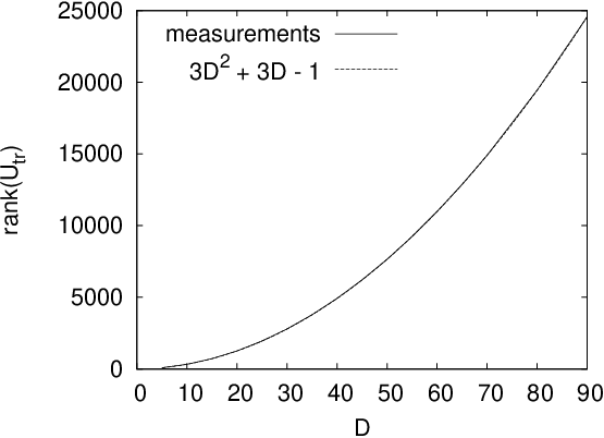
The spectrum of the truncated Koopman operator on this finite functional space of dimension is inside the unit-circle on the complex plane. The side effect of the truncation is that is not invertible, having the rank smaller than the dimension, see Figure 11a. Notice that only non-zero eigenvalues are far enough from the unit circle participate in decay of from the start. We studied the distribution of modulus of eigenvalues denoted by and have found that the probability scales like , see Figure 11b. On the other hand the distribution of eigenvalue modules has singularity at zero of the form .

(a) (b)
It is worthwhile to mention that eigenvalues have higher density near the unit circle. The peak of eigenvalues is with increasing slowly moving to the unit-circle and thereby we observe the squeezing of the spectral gap defined as . The gap in our case is a non-smooth function of . However, due to the condensation, the gap does not have an important dynamical meaning. The number of eigenvalues by magnitude larger than some value is increasing as , where fitted value of the exponent is , see Figure 12a. This scaling can be also applied to eigenvalues near the unit-circle so that behaviour of eigenvalue modules near the circle align for different as we can see in Figure 12b.


(a) (b)
Although the connection between the fidelity and the spectrum of the truncated Koopman operator is clear, we find that the behaviour of eigenvalue modulus with is insufficient to explain the scaling properties of the fidelity.
4 Dynamics of polygons
In this section we consider a heuristic but quite fruitful geometric approach, namely we study the dynamics of the map acting on particular simple subsets of phase space , the polygons. It is easy to verify that all the ingredients of the dynamics preserve polygons, namely maps a polygon to a polygon, and hence its iterates map a polygon to a finite set of several polygons. Furthermore it is possible to make an efficient and accurate numerical algorithm for performing dynamics of polygons by representing them - or their boundaries - in terms of sets of lines.
In the following subsection we describe and apply such explicit construction and the related numerical procedure in order to study the statistical properties of transformed polygons as it emerges from iterating the dynamics for sufficiently long times.
4.1 Statistical properties of polygons
We now consider an arbitrary initial polygon and evolve it with time , . After some time , the set is composed of many, say , pieces. The following main questions are addressed in our numerical experiment:
- •
Do there exist well defined statistical distributions of geometric properties of these little polygonal pieces, such as area, diameter in -direction, diameter in -direction etc., after long time , and do these distributions possess properly defined averages and variances?
- •
What are the scalings of geometric properties of little pieces as grows? Are asymptotic, , statistical distributions universal, i.e. independent of the geometry and volume of the initial set ?
- •
Are these pieces distributed uniformly in phase space , i.e. that the number of pieces inside an arbitrary (‘window’) set with area is, after long time , equal to ?
A computer program has been written which computes an exact evolution of an arbitrary initial polygon in terms of a set of polygons . Affirmative answers to the above questions (for generic, irrational values of parameters ) are strongly suggested by the numerical results which are summarised below. It can be easily shown that any connected piece, say , of has the following properties (which are preserved under time evolution): 11 1 Provided such conditions are imposed on the initial polygon . Otherwise, these properties hold for ever increasing fraction of its little pieces, namely for those whose boundary no longer contains the image of any part of the boundary of the initial set .
- 1.
There exist left-lower and right-upper corner points, , with coordinates and , respectively, such that for arbitrary : , .
- 2.
The boundary of the polygon can be written in terms of two piece-wise linear curves (monotonically increasing in plane) going from to , namely lower and upper boundary. Going from to , the slopes of the straight segments of in plane can be written in terms of an increasing sequence of positive integers , as , while the slopes of the straight lines of are given by a decreasing sequence of positive integers , as
In Figure 13 we show the image of the initial polygon (first plot) in terms of five snapshots (additional five plots) at generic irrational values, , where integer times shown are roughly by a constant factor apart.

Each snapshot is plotted in a renormalised window, around certain reference point (in the center of the phase space, which is here scaled to ), of width and width in order to suggest the scaling.
Observe the statistical similarity of consecutive snapshots!
By repeating the experiment for a smaller initial set the statistical self-similarity persists just the density of little pieces reduces proportionally to the area of the initial set. Figure 14 presents computation for the non-generic (‘weakly-ergodic’) case of (such map has been studied already in Kaplan and Heller (1998)).

We see large temporal and spatial fluctuations in the density of little pieces which may complicate the mechanism of dynamical mixing in this situation. Clearly, general heuristic arguments for the mixing mechanism would not hold for this case. In the other non-generic case and we get similar nonuniform structure with disappearance of some stripes in initial transient time.
We count the number of the little pieces obtained by evolving initial set up to time . In Fig.15 we show for the two generic cases with different initial sets and for a weakly ergodic case.

Always, the growth of is found to be cubic in time after some transient period, with the proportionality constant factor proportional to the area of the initial set
| (33) |
We analyse the statistical distributions of the following geometric measures of little pieces: (i) the area , (ii) the -diameter , (iii) the -diameter , and (iv) the average slope of the piece .
| (34) | |||||
| (35) | |||||
| (36) | |||||
| (37) |
This quantitative results and self-similarity of pieces on the phase space suggest a kind of statistical scaling invariance under the transformation and . Therefore, let us introduce -invariant quantities
| (38) |
Next we investigate the full distributions of scaled quantities . This is done by calculating two different distributions:
- (i)
Cumulative number distributions, equation for the quantity which is one of
(39) - (ii)
Cumulative probability distributions,
(40) where is the step function.
We note that the qualitative features of the number distributions and probability (measure) distributions are essentially the same, so we shall in the following only report numerical results on the former. It has been checked with great numerical accuracy that distributions and are asymptotically (for large ) independent: (i) of time , (ii) of the size and shape of the initial set and (iii) of the particular values of generic irrationals . In Figure 16 we show numerical results on these distributions which suggest several small and large argument asymptotics which are indicated within figures’ labels. It should be noted that the numerical data in Figure 16 can be described even globally quite well by an exponential fit with some exponents .
| (a) |  |
 |
|---|---|---|
| (b) |  |
 |
| (c) |  |
 |
We conjecture and show later in subsection 6.2 for a simplified special case that these distributions (and the scaling) can be derived from the fixed point condition for certain dynamic renormalisation group equations. The later is found for the random triangle model or more precisely for its one-dimensional simplification.
4.2 A Markov approximation
Let us define a finite Markov approximation of the dynamics by the following construction of a transition matrix. We start by the set of two vertical discontinuity lines . They can be viewed as boundaries of two elementary polygons - vertical stripes - which divide the entire torus in two pieces and have no corners. This is just the initial partition that we will be using later to construct a suitable binary coding of the dynamics. Here we discuss only the generic case at parameters , .
Let us now study subsequent images of this set and their union up to integer time :
| (41) |
A set of lines can be considered as a boundary set for a finite set of polygons, let us denote it by . It is obvious that . For any , a set defines a convenient partition of phase space to elements on which we define a probabilistic process in terms of a Markov transition matrix of dimension . Note that if . It is obvious that each element is mapped again onto a single element , provided this element is bounded only by the lines from the set for . For each such the column of transition matrix reads . Hence there acts as a simple permutation. Note that since the number of elements grows as , this happens for a majority of cases, namely only for elements it may happen that their boundary also includes lines from the last image and hence they are cut and split into several elements of . Since the boundary set is a subset of , it is obvious that each such polygon can be cut only once, and hence mapped to at most two polygons, say and . The probabilities are given simply in terms of area measures of image polygons, hence such columns of the transition matrix read
| (42) | |||||
To each split of a polygon we associate the relative splitting strength as
| (43) |
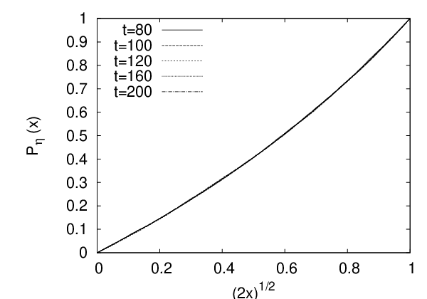
We study the cumulative distribution of splitting strengths, denoted by . In Figure 17a we plot the for different . We notice that small splitting strengths are dominant and the probability density distribution has a square-root singularity at .

(a) (b)
The distribution converges with increasing to its limiting form, which is well fitted by the phenomenological formula
| (44) |
with absolute error and constants and . The first two central moments of the limiting distribution are
| (45) |
In the following we are interested in dynamical and statistical properties of the Markov process for finite times and how they evolve with time . The Markov chain is found to be ergodic and mixing with the spectrum denoted by . In Figure 18 we show two examples of spectra of finite Markov matrices and the distribution of eigenvalue magnitudes which shall be later compared to Markov spectra with respect to an alternative partition coding. Further on, we study the evolution of the spectral gap
| (46) |
and Kolmogorov-Sinai entropy
| (47) |
Because the triangle map is non-hyperbolic, we expect that in the limit the Markov matrix does not have a spectral gap and entropy is equal to zero. This is supported by the numerical results shown in Figure 19. The entropy as a function of time decreases monotonically. Its asymptotic dependence fits well to an algebraic law
| (48) |
Something similar can not be said for the gap, because its dependence on time is not so simple. Nevertheless numerical results suggest that the gap asymptotically decreases inversely proportional with time as
| (49) |


(a) (b)
5 A suitable binary coding
The description in terms of polygons leaves a lot of freedom in the choice of the initial setup. Nevertheless, the dynamical properties of time asymptotics are shown to be only trivially dependent on the initial partition set. In the following we present a description of dynamics based on binary coding of trajectories. In certain chaotic systems, e.g. baker map Arnold and Avez (1989), Lozi and Hénon map (see Cvitanović et al. (1988), D’Alessandro et al. (1991) ), such description is proved to be asymptotically exact. We shall provide evidence that this is the case for our non-hyperbolic system as well.
5.1 Topological complexity of the triangle map
Let be the binary partition of into the half-open rectangles defined as
| (50) |
and we consider the natural coding associated to it. More formally, we let be the coding map defined by
| (51) |
where is the characteristic function of set . One may wonder if is a generating partition, in the sense that
Since horizontal segments remain horizontal during the evolution, whereas arbitrary small vertical segments are linearly stretched while they become asymptotically horizontal, one easily checks that
| (52) |
Therefore, in order that be generating it suffices that the sequence defined in (3) is dense in for all . In the non-generic case, and , this property follows at once from a theorem of Weyl according to which if is a polynomial of degree with real coefficients and at least one of the coefficients is irrational then the sequence is uniformly distributed mod 1 and thus dense, whereas in the generic case this is directly related to the validity of Conjecture 2.
We associate to an individual binary code a set of points defined as
| (53) |
We denote by the set of -admissible words of length , i.e.
| (54) |
The partitions based on the binary partition is then defined as a collection of all non-empty
| (55) |
Note that each is a union of disjoint polygons with horizontal parallel sides, whereas the other two opposite sides are in general not parallel and each has a slope not smaller than (see also below). In Figure 20 snapshots of the iterated partitions for different values of are shown, in fact we plot the set of polygonal boundaries of all elements of , which is just (see equation (41)).


The cardinality of the set , that is
| (56) |
is called the topological complexity function of the pair . In positive entropy systems the cardinality of the set is expected to grow exponentially as
| (57) |
where is the topological entropy. In the non-hyperbolic triangle map we are considering here and therefore we could expect only an algebraic growth. An interesting problem is that of estimating the asymptotic growth of as which is up to a constant factor equal to discussed in Section 4. The numerical experiments (see Figure 21) lead to the conjecture on existence of a positive constant independent of the value of irrational parameters such that
| (58) |
A slightly weaker result was recently proved in Bonanno (2006) and argues that for almost all and one can find two positive constants , such that . Moreover, a similar result is known in rational polygonal billiards Cassaigne et al. (2002). Compatible with this law, at time about elements of the partition get cut into two new pieces, i.e. for about words we have
| (59) |
with both and .

The partition elements are of different sizes (measures) and are decomposed of disjoint polygons, see Figure 22a. We calculate the (heuristic) probability for a partition element being composed of exactly disjoint polygons. An example of the latter is presented in Figure 22b for the generic case. The typical number of polygons in a partition element is one or two, where the second is slightly more favoured. In addition we see that the probability is decreasing approximately stretch-exponentially, . The maximal number of polygons in a partition element appears to be growing approximately proportionally with , but this result is not strongly statistically relevant. The presented properties about decomposition of partitions for the generic case do not change significantly in the non-generic case.


(a) (b)
The areas of partition elements are decreasing with increasing . We study their statistical properties using the cumulative distribution of areas
| (60) |
and cumulative distribution of rescaled areas . In Figure 23 we present in the generic case for different . We see that converges with increasing to an unique distribution with the following behaviour
| (61) |
and
| (62) |
Consequently the average area of partition elements in average decreases as with increasing , which is similar to the polygonal description.


5.2 Transition probability matrix
We are now again going to approximate the dynamics of the triangle map through a probabilistic model i.e Markov chain. The long range correlations in this system prevent (statistical) validity of this description on the long time scale. Nevertheless it gives an useful insight into the properties of the dynamics and the slow mixing decay which we numerically detected in the triangle map.
Similar as above (42) we associate to the triangle map a Markov process Meyn and Tweedie (1995) build on transition probabilities
| (63) |
between elements of the partition . One has
| (64) |
The transition probabilities determine the Markov matrix of our process. Because the cardinality of the partition grows as with increasing , the matrix is sparse for large and therefore can be efficiently stored. The sparseness is increasing with increasing . We recognise that the number of non-zero elements in is equal to
| (65) |
By considering the Markov matrix of the th iterate of the map the number of non-zero elements is . Note that a point with is mapped to , where and . Consequently each column of has at most two nonzero entries denoted by and . We refer to as the splitting strength of the element in labeled by and is defined as
| (66) |
An individual element of the partition is mapped by the Markov matrix usually to another element or its image is split between two elements. We calculate for each element in the free propagation length denoted by i.e. how long it can be evolved by without being split. This time is necessarily finite as the opposite would indicate that the map is non-ergodic. The distributions of free propagation lengths it is defined as
| (67) |
and shown in Figure 24a for different . Properly scaled free propagation lengths reveal that the distribution has an asymptotic form for large
| (68) |
We see that the topology of transitions in the Markov matrix strongly suppresses a long free propagation. The average free length scales with time as , which can be read from (68). The splitting strength strongly varies between partitions. This can be seen in Figure 24b, where we plot the cumulative distributions of splitting strength
| (69) |
for one set of parameters. We see that the variable is almost uniformly distributed and that the distribution of converges with increasing to a form well described by model (44) with and .


(a) (b)
It seems that the limiting distribution is common for all generic cases with the first two central moments reading
| (70) |
Without detailed analysis we could say that the the distribution of splitting strengths in the binary and polygonal description is almost identical.
The eigenvalue spectrum of the Markov matrix is confined to the unit circle. Particularly interesting is the spectral gap between the unit-circle and the second largest eigenvalue. Examples of spectra obtained for different times are shown in Figure 25. We notice a persistent eigenvalue corresponding to the invariant distribution. Other eigenvalues inside the unit-circle move with increasing time toward the unit circle. This can be clearly observed in distribution of eigenvalue amplitudes
| (71) |
and in particular by the spectral gap as a function of time . The general form of the distribution of eigenvalues amplitudes do not change with parameters and . An example is shown in 25. The concentration of eigenvalues increases near to the unit circle and around the origin of the complex plane. Around the origin the distribution has an algebraic singularity, approximately , similarly as in the case of the Koopman operator.


From the Figure 26a we can read that the compact ”cloud” of largest eigenvalues in average converges to the unit circle as . The outermost point defines the spectral gap of the system, which is plotted as a function of time in Figure 26b. We see that the gap decreases with increasing algebraically, nevertheless its functional dependence on time is unclear. The gap in the binary coding is smaller than in the polygonal description. This behaviour is generally expected by coarse graining the partition of Markov matrices, which in our case means grouping polygons in binary coded partition elements. The entropy of the Markov matrix in the binary encoding can be written in the following way
| (72) |
The entropy is bounded from above as
| (73) |
where is the total area of elements of the partition that are split by the action of the map . The number of split partition elements is and their total average area is . Therefore we conclude that and this is numerically verified in Figure 26b.


(a) (b)
We calculate the matrix elements at given by a Monte-Carlo integration using points uniformly sampled over the torus so that . We empirically find that it suffices to have the relative error of the gap in observed time windows smaller than .
Next we consider a class of random Markov matrices of dimension , which mimics known statistical properties of the Markov matrices obtained in the generic case of the triangle map system. We are interested in the asymptotics as . The individual matrix in this class is a perturbed permutation matrix defined as
| (74) |
where is a permutation matrix Heersterman (1990) associated to a random indecomposable permutation , with matrix elements , and represent the perturbation in the expression (74) given by
| (75) |
with being a random permutation. There is only non-zero coefficients , with an average . We estimate the average gap between eigenvalues and the unit circle in these class of Markov matrices using the standard perturbation method Courant and Hilbert (1989). The indecomposible permutation matrix is similar to down-shift permutation matrix
| (76) |
where is just a product of transpositions. The matrix can be diagonalized and its eigensystem is given by
| (77) |
Knowing that the eigensystem of the permutation matrix is with , we find that amplitudes of eigenvalues of matrix in the first order perturbation are
| (78) |
and in the leading order depend only on the coefficients
| (79) |
Following this formula (79) the effective spectral gap for the Markov matrices of the triangle map should scale with time asymptotics as
| (80) |
where , and, because the elements in the rows of matrix can be equally large we take . The results do not give the dependence of the gap in the polygonal and binary encoding of dynamics, but rather a correct time scaling of the distribution of the group of largest eigenvalues in both descriptions.
6 Stochastic models
The deterministic model is found to be a hard system to analyse, and in particular to establish rigorous results. In order to avoid some of the most difficult technical problems, but still to obtain intuitively correct understanding of the dynamics of triangle maps we turn to stochastic models. The stochasticity is introduced in the position of the discontinuity of the triangle map (the cut), which is from analytical point of view, the most problematic.
6.1 Random triangle map
We introduce a stochastic version of the triangle map, called random triangle map, by randomising the position of the discontinuity and thereby preserving essential properties of the deterministic case e.g. the non-hyperbolic nature of the dynamics. The random triangle map is defined as the iteration formula
| (81) | |||||
| (82) |
where is a u.d. random variable. In this system we again introduce the binary coding for a single realisation of the random sequence as it was introduced for the deterministic variant.
We study the behaviour of partitions with time across realisations of the random sequence . The number of partitions in binary coding at some varies strongly with the realisation of the cuts . Nevertheless we find a very simple behaviour of its mean and standard deviation in the generic case:
| (83) |
with being constants and denoting the average over all realisations of . The numerically results are depicted in Figure 27a, where by fitting the data to the power law we find exponents and . We may heuristically expect as this is somehow the largest power we observe theoretically in sequences of such simple maps.


(a) (b)
We conclude that the number of elements of the partitions is asymptotically proportional to similarly as in the deterministic variant. In addition the relative deviation , where , meaning that presented behaviour for the mean value is asymptotically stable. Furthermore we investigate the distribution of and we find a very good agreement with the Gaussian distribution for all
| (84) |
for the rescaled number of elements of the partitions . This is demonstrated in Figure 27b. The form of the distribution and the same scaling of and with time makes us to suspect that should be, for , approximately represented as a sum of independent stochastic variables. Next we take a look a the average distribution of areas of the elements of the partitions in the binary coding. We study the average distribution of areas of elements of the partitions
| (85) |
and average distribution of rescaled areas
| (86) |
over the set of partitions. These two average distributions are not equivalent due to changes to the number elements of the partitions between different realisations of the cuts . In generic case shown in Figure 28 we find that these distributions have similar functional dependence, which seems to have a simple asymptotics at large times reading
| (87) |
The obtained dependence coincides with the dependence in the deterministic case using the binary coding, but due to the computational complexity of the problem we cannot establish the nature of the decay more precisely.


(a) (b)
Next we examine the mixing property in the stochastic model by studying the auto-correlation function of an observable with zero phase-space integral reading
| (88) |
where a trajectory with a given and initial point is denoted by for . In particular, we focus on the first two central moments of the correlations w.r.t. the average over i.e. and . We performed numerical calculations of the two moments using different parameters . The results for the generic case of parameters are shown in Figure 29, whereas for the non-generic case in Figure 30.


(a) (b)
In Figures 29a and 30a we see that the average autocorrelation in the generic and non-generic case decays exponentially
| (89) |
and stretch-exponentially
| (90) |
for large times , respectively. The decay of average correlation is faster than algebraic, which is expected in stochastic systems. In all tested cases we obtain in the random triangle map the same power law decay of the standard deviation of the autocorrelation reading
| (91) |
This is the same power-law decay as the one found for the correlation in generic case of the deterministic triangle map. This behaviour can be clearly seen in figures 29b and 30b. In Subsection 6.3 we clarify this behaviour by showing that the dispersion of correlation is inversely proportional to , which in our case scales as .


(a) (b)
6.2 Random triangle map acting on one-dimensional sets
Here we would like to show that the model of random triangle map can be even simplified and still possesses some interesting features of the (random) triangle map.
In the previous subsection we have analysed distributions of polygon/partition attributes within a stochastic model. The following random model indeed mimics the deterministic triangle map (1) using the polygonal description, if we assume random positions ( coordinates) of the cuts, relative to the positions of a given polygonal piece. In this subsection we show that such analysis can be performed analytically for a special case of a set of degenerate polygons, namely the line segments. We derive explicit results for the distribution of the length of line segments as a function of time.
Let us take initial set to be a vertical line of certain length. Then after time , the image is composed of many short lines, each of which has slope . So, the correct scaled slope variable is a constant which is consistent with the scaling of the general case above (37). Therefore we may continue investigating just one of the quantities, e.g. , while the others are related to it, e.g. . Let be the probability that at time a randomly chosen piece has a horizontal length between and . Vertical size of this piece is , so the total probability that this piece does not get cut in one iteration is . Here all pieces are taken with the statistical weight , so represents a distribution of the number of such pieces. Using elementary probability it is easy to derive the following dynamic evolution integro-difference equation
| (92) |
We are interested in a possible asymptotic scaling solutions of the above equation. Indeed, using the ansatz
| (93) |
for large , the equation (92) is in the leading order in equivalent to an ordinary integro-differential equation
| (94) |
which has a unique solution satisfying the appropriate boundary conditions, . Note that is the scaled number density, , so we have the cumulative distribution,
| (95) |
The first remarkable result of this simplified analysis is the correct scaling variables . In the spirit of the presented simplified analysis we can also express the effective area of a polygon to be proportional to . Then the formula (95) immediately yields the cumulative distribution of the areas reading
| (96) |
The second notable results is that the distributions (95) and (96) are essentially identical, or very close for the areas distribution, to the numerical results in the deterministic triangle map reported in Figure 16.
6.3 Relation for the correlations decay
In the following we present a heuristic derivation of the correlation decay in (random) triangle map using only its basic properties. Let us take two sets of positive measure and consider the correlations of characteristic functions of the sets,
| (97) |
The total number of pieces to which is cut up to time , with average area , see equations (34), (58) and (83), is in all studied cases estimated by
| (98) |
The number of pieces of which map to a test set , and hence contributes to the correlation function (97), is
| (99) |
Assuming that pieces (partitions) are uniformly and pseudo-randomly distributed over the set , the expected standard deviation of is , and an estimated value of the fluctuation of the correlation function reads
| (100) |
for , where we implicitly use that is negligible in comparison to . This is precisely the scaling law which is observed in numerical explorations of the random triangle map. We believe that this elucidates the law of decay of correlations in the (deterministic) triangle map.
7 Conclusions
We presented both theoretical and numerical analysis of a two-parameter family of nonhyperbolic dynamical system related to the classical motion in a polygonally shaped billiard. We formulated several conjectures, and provided strong numerical evidence for their validity, concerning the ergodic behaviour of this family for different sets of parameters values. In particular, we believe that the system is strongly mixing (and thus ergodic) at least in a situation named generic, where both parameters are mutually incommensurate irrationals so that in particular no periodic orbits exist. We also found a kind of mixing behaviour in the case where only the parameter controlling the strength of the cut is irrational whereas is equal to zero. However, the two cases exhibit different mixing behaviours, diffusion properties and periodic orbit structure.
The dynamical properties are studied by means of two different symbolic encoding schemes based on propagating an initial set of polygons and following the two portions of phase space separated by the discontinuity lines, referred to as the polygonal and the binary description, respectively. Using these schemes we numerically deduced several asymptotic scaling properties - for some of which we provided a semi-heuristic analytical explanation. In particular we focused on the spectrum of the Markov transition matrix (in either of the two symbolic descriptions) near to the unit circle and on its spectral gap in relation to the correlation decay. The average convergence of the group of largest eigenvalues to the unit circle as the size of the matrix increases is quantitatively explained by perturbative analysis of a simple random model. We have also briefly studied the Koopman operator associated to the map on a finite dimensional Hilbert space obtained by truncating the Fourier basis. There we found interesting scaling properties of the spectrum and fidelity with respect to the dimension of the space.
Finally, we have introduced a stochastic version of the triangle map which allowed us to obtain some theoretical asymptotic scalings of the distribution of degenerate polygons, thus yielding the decay of correlations observed numerically in the generic case.
This paper presents a bulk of numerical results, along with sparse analytical arguments, on the properties of the triangle map. From the mathematical point of view several important problems remain to be solved. Some of them, in particular the dynamical mechanism underlying the observed strongly mixing behaviour (for some parameter values) of this piecewise parabolic system is a challenging problem in ergodic theory whose solution may require the development of new ideas and techniques.
Acknowledgments
MH thanks for the support by the Department of Mathematics at the University of Bologna, Italy. MH and TP acknowledge support from research grants P1-0044 and J1-7347 of Slovenian Research Agency.
References
- Arnold and Avez (1989) Arnold, V. I., Avez, A., 1989. Ergodic Problems of Classical Mechanics. Addison-Wesley.
- Bonanno (2006) Bonanno, C., 2006. private communication.
- Casati and Prosen (1999) Casati, G., Prosen, T., 1999. Mixing properties of triangular billiards. Phys. Rev. Lett. 83, 4729–32.
- Casati and Prosen (2000) Casati, G., Prosen, T., 2000. Triangle map: a model of quantum chaos. Phys. Rev. Lett. 85, 4261–4264.
- Casati et al. (2005a) Casati, G., Prosen, T., Lan, J., Li, B., 2005a. Universal decay of the classical loschmidt echo of neutrally stable mixing dynamics. Phys. Rev. Lett. 94, 114101.
- Casati et al. (2005b) Casati, G., Tsallis, C., Baldovin, F., 2005b. Linear instability and statistical laws of physics. Europhys. Lett. 72, 355–361.
- Cassaigne et al. (2002) Cassaigne, J., Hubert, P., Troubezkoy, S., 2002. Complexity and growth for polygonal billiards. Ann. Inst. Fourier (Grenoble) 52, 835–847.
- Christiansen and Politi (1996) Christiansen, F., Politi, A., 1996. Symbolic encoding in symplectic maps. Nonlinearity 9, 1623–1640.
- Courant and Hilbert (1989) Courant, R., Hilbert, D., 1989. Methods of Mathematical Physics, Vol. I. John Wiley & Sons.
- Courbage and Hamdan (1997) Courbage, M., Hamdan, D., 1997. Decay of correlations and mixing properties in a dynamical system with zero K-S entropy. Ergod. Th. Dynam. Sys. 17, 87–103.
- Cvitanović et al. (1988) Cvitanović, P., Gunaratne, G. H., Procaccia, I., Aug 1988. Topological and metric properties of Hénon-type strange attractors. Phys. Rev. A 38 (3), 1503–1520.
- D’Alessandro et al. (1991) D’Alessandro, G., Isola, S., Politi, A., 1991. Geometrical properties of the pruning front. Progress in Theoretical Physics 86, 1149.
- Demmel and Hida (2003) Demmel, J., Hida, Y., 2003. Accurate and efficient floating point summation. SIAM J. Sci. Comput. 25, 1214–1248.
- Duarte Queiros (2008) Duarte Queiros, S. M., 2008. On the role of ergodicity and mixing in the central limit theorem for casati-prosen triangle map variables. a numerical experiment. ArXiv e-prints 802.
- Gutkin (1996) Gutkin, E., 1996. Billiards in polygons: Survey of recent results. J. Stat. Phys. 83, 7–26.
- Heersterman (1990) Heersterman, A. R. G., 1990. Matrices and their roots, a textbook of matrix algebra. World Scientific.
- Isola (2006) Isola, S., 2006. Dispersion properties of ergodic translations. International Journal of Mathematics and Mathematical Sciences 2006, Article ID 20568, 1–20.
- Kaplan and Heller (1998) Kaplan, L., Heller, E. J., 1998. Weak quantum ergodicity. Physica D 121, 1–18.
- Katok and Hasselblatt (1995) Katok, A., Hasselblatt, B., 1995. Introduction to the modern theory of dynamical systems. Cambridge University Press, Cambridge.
- Kuipers and Niederreiter (1974) Kuipers, L., Niederreiter, H., 1974. Uniform distribution of sequences. John Wiley and Sons.
- Masur and Tabachnikov (2002) Masur, H., Tabachnikov, S., 2002. Rational billiards and flat structures. In: Handbook of dynamical systems, Vol. 1A. North-Holland, pp. 1015–1089.
- Meyn and Tweedie (1995) Meyn, S., Tweedie, R. L., 1995. Markov chains and Stochastic stability. Springer-Verlag.
- Richens and Berry (1981) Richens, P. J., Berry, M. V., 1981. Pseudo-integrable systems in classical and quantum mechanics. Physica 2D, 495–512.
- Stoer and Bulirsch (2002) Stoer, J., Bulirsch, R., 2002. Introduction to Numerical Analysis, 3rd Edition. Springer Verlag.
- Tabachikov (1995) Tabachikov, S., 1995. Billiards ”Panoramas et Syntheses”. Soc. Math. France.