跳到论文正文
W Papers独立论文阅读器 arXiv:0802.4210 论文正文 计算阅读时间 · 0%
引用这篇论文根据当前论文元数据生成,正式投稿前建议核对。


License: arXiv.org perpetual non-exclusive license
arXiv:0802.4210v3 [astro-ph] 19 Mar 2009

Rotation of Linear Polarization Plane and Circular Polarization from Cosmological Pseudoscalar Fields

Fabio Finellia,b,c, Matteo Galavernid,a,c Affiliation: aINAF-IASF Bologna, Via Gobetti 101, I-40129 Bologna - Italy Affiliation: bINAF/OAB, Osservatorio Astronomico di Bologna, Via Ranzani 1, I-40127 Bologna - Italy Affiliation: cINFN, Sezione di Bologna, Via Irnerio 46, I-40126 Bologna - Italy Affiliation: dDipartimento di Fisica, Università di Ferrara, Via Saragat 1, I-44100 Ferrara - Italy
Abstract

We discuss the rotation of the linear polarization plane and the production of circular polarization generated by a cosmological pseudoscalar field. We compute analytically and numerically the propagation of the Stokes parameters from the last scattering surface for an oscillating and a monotonic decreasing pseudoscalar field. For the models studied in this paper, we show the comparison between the widely used approximation in which the linear polarization rotation angle is constant in time and the exact result.

pacs
95.35.+d, 14.80.Mz

I Introduction

In 1977 R. Peccei and H. Quinn [1] suggested a solution to the strong CP-problem of QCD introducing a new symmetry breaking at a given energy scale faf_{a}. The boson associated with this broken global symmetry was called axion. All the physical properties of this pseudoscalar field strongly depend on the energy scale faf_{a} at which the new symmetry is broken: the particle mass and the coupling constants with other particles are inversely proportional to faf_{a}. Pseudo-Goldstone bosons also arise in many particle physics scenarios [2].

Axions and, in general, other pseudoscalar particles are among the most favoured particle physics candidates for the cold dark matter (CDM) [3, 4, 5]. They interact with photons according to the lagrangian:

ℒi​n​t=−gϕ4​ϕ​Fμ​ν​F~μ​ν,\mathcal{L}_{int}=-\frac{g_{\phi}}{4}\phi F_{\mu\nu}\tilde{F}^{\mu\nu}\,, (1)

where gϕg_{\phi} is the coupling constant, Fμ​νF^{\mu\nu} is the electromagnetic tensor and F~μ​ν≡12​ϵμ​ν​ρ​σ​Fρ​σ\tilde{F}^{\mu\nu}\equiv\frac{1}{2}\epsilon^{\mu\nu\rho\sigma}F_{\rho\sigma} its dual. Many constraints on axion derive from this interaction with photons: laboratory experiments (photon-axion conversion experiments) and astrophysical arguments (stellar evolution of red giants) constrain gϕg_{\phi} to be small. One of the most stringent experimental bound (gϕ<8.8×10⁻²⁰g_{\phi}<8.8\times 10^{-20} eV−1\mbox{eV}^{-1} for ma<0.02m_{a}<0.02 eV) is obtained by the CAST experiment [6] constraining the axion-photon conversion for solar axions. This limit supersedes the one obtained from the duration of the helium burning time in horizontal-branch stars in globular clusters: gϕ≲10−19g_{\phi}\lesssim 10^{-19} eV−1\mbox{eV}^{-1} [4, 7].

In this paper we wish to study in detail the coupling of such a pseudoscalar field with photons. The interaction in Eq. (1) modifies the polarization of an electromagnetic wave propagating along intervening magnetic fields, or through a slowly varying background field ϕ\phi [8]. Here we are interested in the second case, which does not require the presence of a magnetic field (note that in the first case the polarization is also modified in absence of axions, an effect known as Faraday rotation). We consider the time dependent pseudoscalar condensate as dark matter or part of it and study the impact of its time derivative on the polarization of the photons. As a consequence of its coupling with a pseudoscalar field, the plane of linear polarization of light is rotated (cosmological birefringence) [9, 10].

In the case of Cosmic Microwave Background (CMB) photons, we pay attention to the rotation along the path between the last scattering surface (LSS) and the observer, modifying the polarization pattern generated by Thomson scattering at LSS [11]. This rotation induced by the pseudoscalar interaction modifies the gradient and curl of the polarization pattern (EE and BB following [12]), creating BB modes from EE modes. The parity violating nature of the interaction generates non-zero parity-odd correlators (T​BT\,B and E​BE\,B) which would be otherwise vanishing for the standard Gaussian cosmological case [13, 14]. In particular the T​BT\,B power spectrum may be very useful to constrain the coupling constant gϕg_{\phi} between photons and pseudoscalars, since it is larger than the auto and cross power spectra in polarization; in general, these non-standard correlators are already constrained by present data sets [15, 16, 17].

We study two representative examples for the dynamics of a pseudo-Goldstone field behaving as dark matter (see [18] for a pseudoscalar field model of dark energy): the oscillating and a monotonic decreasing behavior. In the latest case we study analytically the problem, whereas in the former numerically and analytically. The case of a field growing linearly in time has been studied in [19]. We compare the polarization power spectra obtained describing the rotation of linear polarization with a time dependent angle with the ones obtained considering a constant rotation angle.

Our paper is organized as follows. We write the relevant equations for the electromagnetic gauge potential coupled to a pseudoscalar field in Section II. We review the Stokes parameters for a monochromatic electromagnetic plane wave and the Boltzmann equation for CMB photons coupled to pseudoscalars in Section III. In Section IV we write the Stokes parameters in terms of the left and right polarizations gauge potential and solve the differential equations for the latter for oscillating behavior of the pseudoscalar field. In a similar way Section V is dedicated to the monotonic behavior of the pseudoscalar field. In Section VI we test the constant rotation angle approximation. We conclude in Section VII. We work in units where the speed of light is equal to one (c=1c=1).

II Electrodynamics Coupled to a Pseudoscalar Field

The lagrangian density ℒ\mathcal{L} for the photons and the pseudoscalar field ϕ\phi is [20] (following the notation of [21]):

ℒ=−14​Fμ​ν​Fμ​ν−12​∇μϕ​∇μϕ−V⁡(ϕ)−gϕ4​ϕ​Fμ​ν​F~μ​ν.\mathcal{L}=-\frac{1}{4}F_{\mu\nu}F^{\mu\nu}-\frac{1}{2}\nabla_{\mu}\phi\nabla^{\mu}\phi-V(\phi)-\frac{g_{\phi}}{4}\phi F_{\mu\nu}\tilde{F}^{\mu\nu}\,. (2)

The Euler-Lagrange equations resulting from this lagrangian are:

□​ϕ≡∇μ∇μ​ϕ\displaystyle\Box\phi\equiv\nabla_{\mu}\nabla^{\mu}\phi =\displaystyle= d​Vd​ϕ+gϕ4​Fμ​ν​F~μ​ν,\displaystyle\frac{dV}{d\phi}+\frac{g_{\phi}}{4}F_{\mu\nu}\tilde{F}^{\mu\nu}\,, (3)
∇μFμ​ν\displaystyle\nabla_{\mu}F^{\mu\nu} =\displaystyle= −gϕ​(∇μϕ)​F~μ​ν,\displaystyle-g_{\phi}(\nabla_{\mu}\phi)\tilde{F}^{\mu\nu}\,, (4)
∇μF~μ​ν\displaystyle\nabla_{\mu}\tilde{F}^{\mu\nu} =\displaystyle= 0.\displaystyle 0\;. (5)

Using the definition of the electromagnetic tensor Fμ​ν≡∇μAν−∇νAμF^{\mu\nu}\equiv\nabla^{\mu}A^{\nu}-\nabla^{\nu}A^{\mu} Eq. (4) becomes:

□​Aν−∇ν(∇μAμ)−Rμν​Aμ=−gϕ2​(∇μϕ)​ϵμνρ​σ​Fρ​σ.\Box A_{\nu}-\nabla_{\nu}\left(\nabla_{\mu}A^{\mu}\right)-{R^{\mu}}_{\nu}A_{\mu}=-\frac{g_{\phi}}{2}(\nabla_{\mu}\phi){{\epsilon^{\mu}}_{\nu}}^{\rho\sigma}F_{\rho\sigma}\;. (6)

The complete antisymmetric tensor contain the determinant of the metric gg and [⋯]\left[\cdots\right] guarantees anti-symmetry in the four indexes [22]:

ϵα​β​γ​δ\displaystyle\epsilon_{\alpha\beta\gamma\delta} =\displaystyle= −g​[α​β​γ​δ],\displaystyle\sqrt{-g}\left[\alpha\beta\gamma\delta\right]\,, (7)
ϵα​β​γ​δ\displaystyle\epsilon^{\alpha\beta\gamma\delta} =\displaystyle= −(−g)−1​[α​β​γ​δ].\displaystyle-\left(\sqrt{-g}\right)^{-1}\left[\alpha\beta\gamma\delta\right]\,. (8)

For a spatially flat Friedmann-Robertson-Walker universe the metric is:

d​s2=−d​t2+a2​(t)​d​𝒙2=a2​(η)​[−d​η2+d​𝒙2],ds^{2}=-dt^{2}+a^{2}(t)d\bm{x}^{2}=a^{2}(\eta)\left[-d\eta^{2}+d\bm{x}^{2}\right]\,, (9)

where tt is the cosmic time, η\eta is conformal time and 𝒙\bm{x} denotes the space coordinates. We consider a plane wave propagating along 𝒏^\bm{\hat{n}} in Coulomb gauge (∇⋅𝑨=0\nabla\cdot\bm{A}=0). If 𝒏^\bm{\hat{n}} is aligned with the zz axis and neglecting the spatial variation of the pseudoscalar field ϕ=ϕ⁡(η)\phi=\phi(\eta), the two relevant components of Eq. (6) are:

Ax′′​(η,z)−∂2Ax​(η,z)∂z2\displaystyle A_{x}^{\prime\prime}\left(\eta,z\right)-\frac{\partial^{2}A_{x}\left(\eta,z\right)}{\partial z^{2}} =\displaystyle= gϕ​ϕ′​∂Ay​(η,z)∂z,\displaystyle g_{\phi}\phi^{\prime}\frac{\partial A_{y}\left(\eta,z\right)}{\partial z}\,, (10)
Ay′′​(η,z)−∂2Ay​(η,z)∂z2\displaystyle A_{y}^{\prime\prime}\left(\eta,z\right)-\frac{\partial^{2}A_{y}\left(\eta,z\right)}{\partial z^{2}} =\displaystyle= −gϕ​ϕ′​∂Ax​(η,z)∂z.\displaystyle-g_{\phi}\phi^{\prime}\frac{\partial A_{x}\left(\eta,z\right)}{\partial z}\,. (11)

Defining Fourier transform as A~x,y​(k,η)=(2​π)−1​∫ei​k​z​Ax,y​(η,z)​𝑑z\tilde{A}_{x,y}(k,\eta)=(2\pi)^{-1}\int e^{ikz}A_{x,y}(\eta,z)dz the previous equations become:

A~x′′​(k,η)+k2​A~x​(k,η)+gϕ​ϕ′​i​k​A~y​(k,η)=0,\displaystyle\tilde{A}_{x}^{\prime\prime}(k,\eta)+k^{2}\tilde{A}_{x}(k,\eta)+g_{\phi}\phi^{\prime}ik\tilde{A}_{y}(k,\eta)=0\,, (12)
A~y′′​(k,η)+k2​A~y​(k,η)−gϕ​ϕ′​i​k​A~x​(k,η)=0.\displaystyle\tilde{A}_{y}^{\prime\prime}(k,\eta)+k^{2}\tilde{A}_{y}(k,\eta)-g_{\phi}\phi^{\prime}ik\tilde{A}_{x}(k,\eta)=0\,. (13)

where kk is the Fourier conjugate of zz.
These equations can be decoupled introducing A~±​(k,η)=A~x​(k,η)±i​A~y​(k,η)\tilde{A}_{\pm}(k,\eta)=\tilde{A}_{x}(k,\eta)\pm i\tilde{A}_{y}(k,\eta), left and right components of the electro-magnetic vector potential:

A~±′′​(k,η)+[k2±gϕ​ϕ′​k]​A~±​(k,η)=0.\tilde{A}_{\pm}^{\prime\prime}(k,\eta)+\left[k^{2}\pm g_{\phi}\phi^{\prime}k\right]\tilde{A}_{\pm}(k,\eta)=0\,. (14)

III Standard Review of Stokes Parameters and Boltzmann Equation

III.1 Stokes Parameters

The complex electric field vector for a plane wave propagating along 𝒛^\bm{\hat{z}} direction at a point (x,y)(x,y) in some transverse plane z=z0z=z_{0} is:

𝑬\displaystyle\bm{E} =\displaystyle= (Ex​(t),Ey​(t))\displaystyle\left(E_{x}(t)\,,E_{y}(t)\right) (15)
=\displaystyle= [𝒆^𝒙​εx​(t)​ei​φx​(t)+𝒆^𝒚​εy​(t)​ei​φy​(t)]​e−i​k​t,\displaystyle\left[\bm{\hat{e}_{x}}\varepsilon_{x}(t)e^{i\varphi_{x}(t)}+\bm{\hat{e}_{y}}\varepsilon_{y}(t)e^{i\varphi_{y}(t)}\right]e^{-ikt}\,,

where the physical quantity is the real part of 𝑬\bm{E}. For a spatially flat Friedmann-Robertson-Walker metric the relation between the electromagnetic tensor and the physical fields is:

Fμ​ν=a⁡(η)​(0−Ex−Ey−EzEx0Bz−ByEy−Bz0BxEzBy−Bx0).F_{\mu\nu}=a(\eta)\left(\begin{array}[]{cccc}0&-E_{x}&-E_{y}&-E_{z}\\ E_{x}&0&B_{z}&-B_{y}\\ E_{y}&-B_{z}&0&B_{x}\\ E_{z}&B_{y}&-B_{x}&0\end{array}\right)\,. (16)

In general we consider quasi-monochromatic waves: the amplitudes (εx​(t)\varepsilon_{x}(t) and εy​(t)\varepsilon_{y}(t)) and the phases (φx​(t)\varphi_{x}(t) and φy​(t)\varphi_{y}(t)) are slowly varying functions of time respect to the inverse frequency of the wave.

The Stokes parameters I,Q,U​and​VI,\,Q,\,U\,\mbox{and}\,V are defined as:

I\displaystyle I ≡\displaystyle\equiv 1a2​(⟨Ex∗​(t)​Ex​(t)⟩+⟨Ey∗​(t)​Ey​(t)⟩),\displaystyle\frac{1}{a^{2}}\left(\left\langle E^{*}_{x}(t)E_{x}(t)\right\rangle+\left\langle E^{*}_{y}(t)E_{y}(t)\right\rangle\right)\,, (17)
Q\displaystyle Q ≡\displaystyle\equiv 1a2​(⟨Ex∗​(t)​Ex​(t)⟩−⟨Ey∗​(t)​Ey​(t)⟩),\displaystyle\frac{1}{a^{2}}\left(\left\langle E^{*}_{x}(t)E_{x}(t)\right\rangle-\left\langle E^{*}_{y}(t)E_{y}(t)\right\rangle\right)\,, (18)
U\displaystyle U ≡\displaystyle\equiv 1a2​(⟨Ex∗​(t)​Ey​(t)⟩+⟨Ey∗​(t)​Ex​(t)⟩)\displaystyle\frac{1}{a^{2}}\left(\left\langle E^{*}_{x}(t)E_{y}(t)\right\rangle+\left\langle E^{*}_{y}(t)E_{x}(t)\right\rangle\right) (19)
=\displaystyle= 2a2​⟨εx​εy​cos⁡(φx−φy)⟩,\displaystyle\frac{2}{a^{2}}\left\langle\varepsilon_{x}\varepsilon_{y}\cos\left(\varphi_{x}-\varphi_{y}\right)\right\rangle\,,
V\displaystyle V ≡\displaystyle\equiv −ia2​(⟨Ex∗​(t)​Ey​(t)⟩−⟨Ey∗​(t)​Ex​(t)⟩)\displaystyle-\frac{i}{a^{2}}\left(\left\langle E^{*}_{x}(t)E_{y}(t)\right\rangle-\left\langle E^{*}_{y}(t)E_{x}(t)\right\rangle\right) (20)
=\displaystyle= 2a2​⟨εx​εy​sin⁡(φx−φy)⟩.\displaystyle\frac{2}{a^{2}}\left\langle\varepsilon_{x}\varepsilon_{y}\sin\left(\varphi_{x}-\varphi_{y}\right)\right\rangle.

where ⟨⋯⟩\left<\cdots\right> denote the ensemble average, the average over all possible realizations of a given quasi-monochromatic wave. For a pure monochromatic wave ensemble averages can be omitted and the wave is completely polarized:

I2−Q2−U2−V2=0.I^{2}-Q^{2}-U^{2}-V^{2}=0\,. (21)

The parameter II gives the total intensity of the radiation, QQ and UU describe linear polarization and VV circular polarization. Linear polarization can also be characterized through a vector of modulus:

PL≡Q2+U2,P_{L}\equiv\sqrt{Q^{2}+U^{2}}\,, (22)

and an angle θ\theta, defined as:

θ≡12​arctan⁡UQ.\theta\equiv\frac{1}{2}\arctan\frac{U}{Q}\,. (23)

It is important to underline that II and VV are physical observables, since they are independent on the particular orientation of the reference frame in the plane perpendicular to the direction of propagation 𝒏^\bm{\hat{n}}, while QQ and UU depend on the orientation of this basis [23]. After a rotation of the reference frame of an angle θ\theta (R⁡(θ)R(\theta)) they transform according to:

Q⟶R⁡(θ)Q​cos⁡(2​θ)+U​sin⁡(2​θ),U⟶R⁡(θ)−Q​sin⁡(2​θ)+U​cos⁡(2​θ).\begin{array}[]{ccc}Q&\stackrel{{\scriptstyle R(\theta)}}{{\longrightarrow}}&Q\cos(2\theta)+U\sin(2\theta)\,,\\ U&\stackrel{{\scriptstyle R(\theta)}}{{\longrightarrow}}&-Q\sin(2\theta)+U\cos(2\theta)\,.\end{array} (24)

Also linear polarization, like total intensity and circular polarization, can be described through quantities independent on the orientation of the reference frame in the plane perpendicular to the direction of propagation of the wave. In the context of CMB anisotropies, the linear polarization vector field is usually described in terms of a gradient-like component (E mode) and of a curl-like component (B mode).

In a similar way it is possible to describe the electric vector field in the x−yx-y plane through a superposition of left and right circular polarized waves defining:

𝒆^+≡𝒆^𝒙+i​𝒆^𝒚2and𝒆^−≡𝒆^𝒙−i​𝒆^𝒚2.\displaystyle\bm{\hat{e}_{+}}\equiv\frac{\bm{\hat{e}_{x}}+i\bm{\hat{e}_{y}}}{\sqrt{2}}\qquad\mbox{and}\qquad\bm{\hat{e}_{-}}\equiv\frac{\bm{\hat{e}_{x}}-i\bm{\hat{e}_{y}}}{\sqrt{2}}\,. (25)

In this new basis:

I\displaystyle I ≡\displaystyle\equiv 1a2​(⟨E+∗​(t)​E+​(t)⟩+⟨E−∗​(t)​E−​(t)⟩),\displaystyle\frac{1}{a^{2}}\left(\left\langle E^{*}_{+}(t)E_{+}(t)\right\rangle+\left\langle E^{*}_{-}(t)E_{-}(t)\right\rangle\right)\,, (26)
Q\displaystyle Q ≡\displaystyle\equiv 1a2​(⟨E+∗​(t)​E−​(t)⟩+⟨E−∗​(t)​E+​(t)⟩)\displaystyle\frac{1}{a^{2}}\left(\left\langle E^{*}_{+}(t)E_{-}(t)\right\rangle+\left\langle E^{*}_{-}(t)E_{+}(t)\right\rangle\right) (27)
=\displaystyle= 2a2​⟨ε+​ε−​cos⁡(φ+−φ−)⟩,\displaystyle\frac{2}{a^{2}}\left\langle\varepsilon_{+}\varepsilon_{-}\cos\left(\varphi_{+}-\varphi_{-}\right)\right\rangle\,,
U\displaystyle U ≡\displaystyle\equiv −ia2​(⟨E+∗​(t)​E−​(t)⟩−⟨E−∗​(t)​E+​(t)⟩)\displaystyle-\frac{i}{a^{2}}\left(\left\langle E^{*}_{+}(t)E_{-}(t)\right\rangle-\left\langle E^{*}_{-}(t)E_{+}(t)\right\rangle\right) (28)
=\displaystyle= 2a2​⟨ε+​ε−​sin⁡(φ+−φ−)⟩,\displaystyle\frac{2}{a^{2}}\left\langle\varepsilon_{+}\varepsilon_{-}\sin\left(\varphi_{+}-\varphi_{-}\right)\right\rangle\,,
V\displaystyle V ≡\displaystyle\equiv 1a2​(⟨E+∗​(t)​E+​(t)⟩−⟨E−∗​(t)​E−​(t)⟩).\displaystyle\frac{1}{a^{2}}\left(\left\langle E^{*}_{+}(t)E_{+}(t)\right\rangle-\left\langle E^{*}_{-}(t)E_{-}(t)\right\rangle\right)\,. (29)

The relation between the vector potential and the electric field for a wave propagating in a charge-free region is:

𝑬=−∂𝑨∂t=−𝑨′a,\bm{E}=-\frac{\partial\bm{A}}{\partial t}=-\frac{\bm{A}^{\prime}}{a}\,, (30)

According to definition given in the previous section the Stokes Parameters in terms of the vector potential are:

I\displaystyle I =\displaystyle= 1a4​(⟨A+′⁣∗​A+′⟩+⟨A−′⁣∗​A−′⟩),\displaystyle\frac{1}{a^{4}}\left(\left<A_{+}^{\prime*}A_{+}^{\prime}\right>+\left<A_{-}^{\prime*}A_{-}^{\prime}\right>\right)\,, (31)
Q\displaystyle Q =\displaystyle= 1a4​(⟨A+′⁣∗​A−′⟩+⟨A−′⁣∗​A+′⟩)\displaystyle\frac{1}{a^{4}}\left(\left<A_{+}^{\prime*}A_{-}^{\prime}\right>+\left<A_{-}^{\prime*}A_{+}^{\prime}\right>\right) (32)
=\displaystyle= 2a4​ℜ⁡(⟨A+′⁣∗​A−′⟩),\displaystyle\frac{2}{a^{4}}\Re\left(\left<A_{+}^{\prime*}A_{-}^{\prime}\right>\right)\,,
U\displaystyle U =\displaystyle= −ia4​(⟨A+′⁣∗​A−′⟩−⟨A−′⁣∗​A+′⟩)\displaystyle-\frac{i}{a^{4}}\left(\left<A_{+}^{\prime*}A_{-}^{\prime}\right>-\left<A_{-}^{\prime*}A_{+}^{\prime}\right>\right) (33)
=\displaystyle= 2a4​ℑ⁡(⟨A+′⁣∗​A−′⟩),\displaystyle\frac{2}{a^{4}}\Im\left(\left<A_{+}^{\prime*}A_{-}^{\prime}\right>\right)\,,
V\displaystyle V =\displaystyle= 1a4​(⟨A+′⁣∗​A+′⟩−⟨A−′⁣∗​A−′⟩).\displaystyle\frac{1}{a^{4}}\left(\left<A_{+}^{\prime*}A_{+}^{\prime}\right>-\left<A_{-}^{\prime*}A_{-}^{\prime}\right>\right)\,. (34)

As we shall see in more detail in the following section, the coupling to a cosmological pseudoscalar field induce a physical time-dependent rotation of the plane of linear polarization along the line of sight, described by:

Q′=2​θ′​(η)​UandU′=−2​θ′​(η)​Q,Q^{\prime}=2\theta^{\prime}(\eta)U\quad\mbox{and}\quad U^{\prime}=-2\theta^{\prime}(\eta)Q\,, (35)

whose solution is:

Q=Qi​cos⁡2​θ+Ui​sin⁡2​θ,U=−Qi​sin⁡2​θ+Ui​cos⁡2​θ.\begin{array}[]{ccc}Q&=&Q_{i}\cos 2\theta+U_{i}\sin 2\theta\,,\\ U&=&-Q_{i}\sin 2\theta+U_{i}\cos 2\theta\,.\end{array} (36)

where Qi,UiQ_{i}\,,U_{i} are the Stokes parameters at initial time which would be otherwise unchanged in absence of the interaction with the pseudoscalar field.

III.2 Boltzmann Equation and cosmological birefringence

In the Boltzmann equations for linear polarization of the radiation density contrast averaged over momenta contains a mixing term:

2​θ′=g​ϕ′,2\theta^{\prime}=g\phi^{\prime}\,, (37)

due to the pseudoscalar interaction [11]; the Boltzmann equation for spin-2 functions Q±i​UQ\pm iU is:

ΔQ±i​U′​(k,η)+i​k​μ​ΔQ±i​U​(k,η)\displaystyle\Delta^{\prime}_{Q\pm iU}(k,\eta)+ik\mu\Delta_{Q\pm iU}(k,\eta)
=−ne​σT​a​(η)​[ΔQ±i​U​(k,η)+∑m6​π5​Ym2±2​SP(m)​(k,η)]\displaystyle=-n_{e}\sigma_{T}a(\eta)\left[\Delta_{Q\pm iU}(k,\eta)+\sum_{m}\sqrt{\frac{6\pi}{5}}{}_{\pm 2}Y_{2}^{m}S_{P}^{(m)}(k,\eta)\right]
∓i​2​θ′​(η)​ΔQ±i​U​(k,η).\displaystyle\quad\mp i2\theta^{\prime}(\eta)\Delta_{Q\pm iU}(k,\eta)\,. (38)

where μ\mu is the cosine of the angle between the CMB photon direction and the Fourier wave vector, nen_{e} is the number density of free electrons, σT\sigma_{T} is the Thomson cross section, Ym2s{}_{s}Y_{2}^{m} are spherical harmonics with spin-weight ss, and SP(m)​(k,η)S_{P}^{(m)}(k,\eta) is the source term for generating linear polarization reported in [24] (m=0,±1,±2m=0,\,\pm 1,\,\pm 2 corresponds respectively to scalar, vector, and tenor perturbations):

SP(m)​(k,η)=ΔT​2(m)​(k,η)+12​6​Δ+,2(m)​(k,η)+12​6​Δ−,2(m)​(k,η).S_{P}^{(m)}(k,\eta)=\Delta^{(m)}_{T2}(k,\eta)+12\sqrt{6}\Delta_{+\,,2}^{(m)}(k,\eta)+12\sqrt{6}\Delta_{-\,,2}^{(m)}(k,\eta)\,. (39)

ΔT​l(m)\Delta^{(m)}_{Tl} and Δ±,l(m)\Delta^{(m)}_{\pm\,,l} are the Fourier transforms of the coefficients of the following series:

ΔT​(𝐱,𝐧^,η)\displaystyle\Delta_{T}({\bf x},{\bf\hat{n}},\eta)
=∑l​m(−i)l​4​π​(2​l+1)​ΔT​l(m)​(𝐱,η)​Ylm​(𝐧^),\displaystyle\;=\sum_{l\,m}(-i)^{l}\sqrt{4\pi(2l+1)}\Delta^{(m)}_{Tl}({\bf x},\eta)Y_{l}^{m}({\bf\hat{n}})\,, (40)
ΔQ±i​U​(𝐱,𝐧^,η)\displaystyle\Delta_{Q\pm iU}({\bf x},{\bf\hat{n}},\eta)
=∑l​m(−i)l​4​π​(2​l+1)​Δ±,ℓ(m)​(𝐱,η)​Yml±2​(𝐧^),\displaystyle\;=\sum_{l\,m}(-i)^{l}\sqrt{4\pi(2l+1)}\Delta^{(m)}_{\pm\,,\ell}({\bf x},\eta)\,{}_{\pm 2}Y_{l}^{m}({\bf\hat{n}})\,, (41)

Note that Eq. (38) corrects some typos in Eq. (1) of Ref. [18].

The quantity ΔQ±i​U\Delta_{Q\pm iU} is related to the rotation invariant polarization fields ΔE\Delta_{E} and ΔB\Delta_{B} through the spin raising (∂′\;\raise 1.0pt\hbox{${}^{\prime}$}\hskip-6.0pt\partial\;) and lowering (∂′¯\;\overline{\raise 1.0pt\hbox{${}^{\prime}$}\hskip-6.0pt\partial}\;) operators:

ΔE\displaystyle\Delta_{E} ≡\displaystyle\equiv −12​(∂′¯2​ΔQ+i​U+∂2′⁡ΔQ−i​U),\displaystyle-\frac{1}{2}\left(\;\overline{\raise 1.0pt\hbox{${}^{\prime}$}\hskip-6.0pt\partial}\;^{2}\Delta_{Q+iU}+\;\raise 1.0pt\hbox{${}^{\prime}$}\hskip-6.0pt\partial\;^{2}\Delta_{Q-iU}\right)\,, (42)
ΔB\displaystyle\Delta_{B} ≡\displaystyle\equiv −i2​(∂′¯2​ΔQ+i​U−∂2′⁡ΔQ−i​U).\displaystyle-\frac{i}{2}\left(\;\overline{\raise 1.0pt\hbox{${}^{\prime}$}\hskip-6.0pt\partial}\;^{2}\Delta_{Q+iU}-\;\raise 1.0pt\hbox{${}^{\prime}$}\hskip-6.0pt\partial\;^{2}\Delta_{Q-iU}\right)\,. (43)

Following the line of sight strategy for scalar perturbations we obtain, in agreement with Ref. [18]:

ΔT​(k,η0)\displaystyle\Delta_{T}(k,\eta_{0}) =\displaystyle= ∫ηrecη0d​η​g​(η)​ST​(k,η)​jℓ​(k​η0−k​η),\displaystyle\int_{\eta_{\rm rec}}^{\eta_{0}}d\eta\,g(\eta)S_{T}(k,\eta)j_{\ell}(k\eta_{0}-k\eta)\,, (44)
ΔE​(k,η0)\displaystyle\Delta_{E}(k,\eta_{0}) =\displaystyle= ∫ηrecη0d​η​g​(η)​SP(0)​(k,η)​jℓ​(k​η0−k​η)(k​η0−k​η)2​cos⁡[2​θ​(η)],\displaystyle\int_{\eta_{\rm rec}}^{\eta_{0}}d\eta\,g(\eta)S_{P}^{(0)}(k,\eta)\frac{j_{\ell}(k\eta_{0}-k\eta)}{\left(k\eta_{0}-k\eta\right)^{2}}\cos\left[2\theta(\eta)\right]\,, (45)
ΔB​(k,η0)\displaystyle\Delta_{B}(k,\eta_{0}) =\displaystyle= ∫ηrecη0d​η​g​(η)​SP(0)​(k,η)​jℓ​(k​η0−k​η)(k​η0−k​η)2​sin⁡[2​θ​(η)].\displaystyle\int_{\eta_{\rm rec}}^{\eta_{0}}d\eta\,g(\eta)S_{P}^{(0)}(k,\eta)\frac{j_{\ell}(k\eta_{0}-k\eta)}{\left(k\eta_{0}-k\eta\right)^{2}}\sin\left[2\theta(\eta)\right]\,. (46)

where g⁡(η)g(\eta) is the visibility function, ST​(k,η)S_{T}(k,\eta) is the sorce term for temperature anisotropies, ù and jℓj_{\ell} is the spherical Bessel function. The polarization CℓC_{\ell} auto- and cross-spectra are given by:

CℓE​E\displaystyle C_{\ell}^{EE} =\displaystyle= (4​π)2​9​(ℓ+2)!16​(ℓ−2)!​∫k2​𝑑k​[ΔE​(k,η0)]2,\displaystyle\left(4\pi\right)^{2}\frac{9\left(\ell+2\right)!}{16\left(\ell-2\right)!}\int k^{2}dk\,\left[\Delta_{E}(k,\eta_{0})\right]^{2}\,, (47)
CℓB​B\displaystyle C_{\ell}^{BB} =\displaystyle= (4​π)2​9​(ℓ+2)!16​(ℓ−2)!​∫k2​𝑑k​[ΔB​(k,η0)]2,\displaystyle\left(4\pi\right)^{2}\frac{9\left(\ell+2\right)!}{16\left(\ell-2\right)!}\int k^{2}dk\,\left[\Delta_{B}(k,\eta_{0})\right]^{2}\,, (48)
CℓE​B\displaystyle C_{\ell}^{EB} =\displaystyle= (4​π)2​9​(ℓ+2)!16​(ℓ−2)!​∫k2​𝑑k​ΔE​(k,η0)​ΔB​(k,η0),\displaystyle\left(4\pi\right)^{2}\frac{9\left(\ell+2\right)!}{16\left(\ell-2\right)!}\int k^{2}dk\,\Delta_{E}(k,\eta_{0})\Delta_{B}(k,\eta_{0})\,, (49)
CℓT​E\displaystyle C_{\ell}^{TE} =\displaystyle= (4​π)2​9​(ℓ+2)!16​(ℓ−2)!​∫k2​𝑑k​ΔT​(k,η0)​ΔE​(k,η0),\displaystyle\left(4\pi\right)^{2}\sqrt{\frac{9\left(\ell+2\right)!}{16\left(\ell-2\right)!}}\int k^{2}dk\,\Delta_{T}(k,\eta_{0})\Delta_{E}(k,\eta_{0})\,, (50)
CℓT​B\displaystyle C_{\ell}^{TB} =\displaystyle= (4​π)2​9​(ℓ+2)!16​(ℓ−2)!​∫k2​𝑑k​ΔT​(k,η0)​ΔB​(k,η0).\displaystyle\left(4\pi\right)^{2}\sqrt{\frac{9\left(\ell+2\right)!}{16\left(\ell-2\right)!}}\int k^{2}dk\,\Delta_{T}(k,\eta_{0})\Delta_{B}(k,\eta_{0})\,. (51)

In the approximation in which θ=θ¯\theta=\bar{\theta}, with θ¯\bar{\theta} constant in time, Eqs. (45) and (46) simplify since cos⁡[2​θ¯],sin⁡[2​θ¯]\cos[2\bar{\theta}]\,,\sin[2\bar{\theta}] can be extracted from the integral along the line of sight and:

ΔEo​b​s\displaystyle\Delta_{E}^{obs} =\displaystyle= ΔE​(θ=0)​cos⁡(2​θ¯),\displaystyle\Delta_{E}(\theta=0)\,\cos(2\bar{\theta})\,, (52)
ΔBo​b​s\displaystyle\Delta_{B}^{obs} =\displaystyle= ΔE​(θ=0)​sin⁡(2​θ¯),\displaystyle\Delta_{E}(\theta=0)\,\sin(2\bar{\theta})\,, (53)

and the power spectra are given by [11, 15]:

CℓE​E,o​b​s\displaystyle C_{\ell}^{EE,obs} =\displaystyle= CℓE​E​cos2⁡(2​θ¯),\displaystyle C_{\ell}^{EE}\cos^{2}(2\bar{\theta})\,, (54)
CℓB​B,o​b​s\displaystyle C_{\ell}^{BB,obs} =\displaystyle= CℓE​E​sin2⁡(2​θ¯),\displaystyle C_{\ell}^{EE}\sin^{2}(2\bar{\theta})\,, (55)
CℓE​B,o​b​s\displaystyle C_{\ell}^{EB,obs} =\displaystyle= 12​CℓE​E​sin⁡(4​θ¯),\displaystyle\frac{1}{2}C_{\ell}^{EE}\sin(4\bar{\theta})\,, (56)
CℓT​E,o​b​s\displaystyle C_{\ell}^{TE,obs} =\displaystyle= CℓT​E​cos⁡(2​θ¯),\displaystyle C_{\ell}^{TE}\cos(2\bar{\theta})\,, (57)
CℓT​B,o​b​s\displaystyle C_{\ell}^{TB,obs} =\displaystyle= CℓT​E​sin⁡(2​θ¯).\displaystyle C_{\ell}^{TE}\sin(2\bar{\theta})\,. (58)

The expression for θ¯\bar{\theta} to insert in Eqs. (52-58) is:

θ¯=gϕ2​[ϕ⁡(η0)−ϕ⁡(ηrec)].\bar{\theta}=\frac{g_{\phi}}{2}\left[\phi(\eta_{0})-\phi(\eta_{\rm rec})\right]\,. (59)

Several limits on the constant rotation angle θ¯\bar{\theta} have been already obtained using current observation of CMBP (see Tab. 1).

Data set θ¯​(2​σ)​[deg]\bar{\theta}\;(2\sigma)\;\mbox{[deg]}
WMAP3 and Boomerang (B03) [15] −13.7<θ¯<1.9-13.7<\bar{\theta}<1.9
WMAP3 [16] −8.5<θ¯<3.5-8.5<\bar{\theta}<3.5
WMAP5 [17] −5.9<θ¯<2.4-5.9<\bar{\theta}<2.4
QUaD [25] −1.2<θ¯<3.9-1.2<\bar{\theta}<3.9
Table 1: Constraints on linear polarization rotation θ¯\bar{\theta} in the constant angle approximation.

This time independent rotation angle approximation is an operative approximation which allows to write Eqs. (53), is clearly inconsistent since for θ=const\theta=\mbox{const} the term proportional to θ′\theta^{\prime} in the Boltzmann equation (38) vanishes and therefore there is no rotation of the linear polarization plane. See Figs. 6 and 7 for a comparison of this approximation with a full Boltzmann description of the birefringence effect for a dynamical pseudoscalar field.

IV Cosine-type potential

In this section we assume that dark matter is given by massive axions, ϕ\phi is governed by the potential [3]:

V⁡(ϕ)=m2​fa2N2​(1−cos⁡ϕ​Nfa),V(\phi)=m^{2}\frac{f_{a}^{2}}{N^{2}}\left(1-\cos\frac{\phi N}{f_{a}}\right)\,, (60)

where NN is the color anomaly of the Peccei-Quinn symmetry. Here we are interested in the regime where the axion field oscillates near the minimum of the potential (for simplicity we shall consider N=1N=1 in the following): ϕ/fa≪1\phi/f_{a}\ll 1 and the potential can be approximated with V⁡(ϕ)≃m2​ϕ2/2V(\phi)\simeq m^{2}\phi^{2}/2. In this case ϕ⁡(t)\phi(t) satisfies the equation:

ϕ¨+3​H​ϕ˙+m2​ϕ=0.\ddot{\phi}+3H\dot{\phi}+m^{2}\phi=0\,. (61)

When m>3​Hm>3H the scalar field begins to oscillate, and the solution in a matter dominated universe (a˙/a=2/3​t\dot{a}/a=2/3t) is [26]:

ϕ(t)=t−1/2[c1J1/2(mt)+c2J−1/2(mt)]\displaystyle\phi(t)=t^{-1/2}\left[c_{1}J_{1/2}(mt)+c_{2}J_{-1/2}(mt)\right]
≃m​t≫1ϕ0m​t​sin⁡(m​t),\displaystyle\stackrel{{\scriptstyle mt\gg 1}}{{\simeq}}\frac{\phi_{0}}{mt}\sin(mt)\,, (62)

where the time-independent coefficients of the Bessel functions c1,c2c_{1}\,,c_{2} depend on the initial conditions.

The averaged energy and pressure densities associated with the field are:

ρϕ¯\displaystyle\overline{\rho_{\phi}} =\displaystyle= ϕ˙2¯2+12​m2​ϕ¯2≃m​t≫1ϕ022​t2​[1+𝒪​(1m​t)2],\displaystyle\frac{\overline{\dot{\phi}^{2}}}{2}+\frac{1}{2}m^{2}\overline{\phi}^{2}\stackrel{{\scriptstyle mt\gg 1}}{{\simeq}}\frac{\phi_{0}^{2}}{2t^{2}}\left[1+\mathcal{O}\left(\frac{1}{mt}\right)^{2}\right]\,, (63)
Pϕ¯\displaystyle\overline{P_{\phi}} =\displaystyle= ϕ˙2¯2−12​m2​ϕ¯2≃m​t≫1ϕ022​t2×𝒪​(1m​t)2,\displaystyle\frac{\overline{\dot{\phi}^{2}}}{2}-\frac{1}{2}m^{2}\overline{\phi}^{2}\stackrel{{\scriptstyle mt\gg 1}}{{\simeq}}\frac{\phi_{0}^{2}}{2t^{2}}\times\mathcal{O}\left(\frac{1}{mt}\right)^{2}\,, (64)

where ¯\bar{} denotes the average over an oscillation period of the axion condensate. Note that we are implicitly assuming that the pseudoscalar field is homogeneous. In the context of axion physics, this means that in our observable universe we have just one value for the misalignment angle, which means that the PQ symmetry has occurred before or during inflation.

We fix the constant ϕ0\phi_{0} comparing ρϕ\rho_{\phi} with the energy density in a matter dominated universe:

ρM=3​H2​Mpl28​π=Mpl26​π​t2⟹ϕ0=Mpl3​π,\rho_{M}=\frac{3H^{2}M_{\mathrm{pl}}^{2}}{8\pi}=\frac{M_{\mathrm{pl}}^{2}}{6\pi t^{2}}\quad\Longrightarrow\quad\phi_{0}=\frac{M_{\mathrm{pl}}}{\sqrt{3\pi}}\,, (65)
ϕ⁡(t)≃Mpl3​π​m​t​sin⁡(m​t),\phi(t)\simeq\frac{M_{\mathrm{pl}}}{\sqrt{3\pi}mt}\sin(mt)\,, (66)

where Mpl≃1.22×10¹⁹M_{\mathrm{pl}}\simeq 1.22\times 10^{19} GeV is the Planck mass.

Using the relation between cosmic and conformal time in a universe of matter:

t=η03​(ηη0)3,t=\frac{\eta_{0}}{3}\left(\frac{\eta}{\eta_{0}}\right)^{3}\,, (67)

we find the following approximation for ϕ⁡(η)\phi(\eta):

ϕ⁡(η)≃3π​Mplm​η0​(ηη0)3​sin⁡[m​η03​(ηη0)3],\phi(\eta)\simeq\sqrt{\frac{3}{\pi}}\frac{M_{\mathrm{pl}}}{m\eta_{0}\left(\frac{\eta}{\eta_{0}}\right)^{3}}\sin\left[m\frac{\eta_{0}}{3}\left(\frac{\eta}{\eta_{0}}\right)^{3}\right]\,, (68)

and

ϕ′​(η)≃3π​Mplη\displaystyle\phi^{\prime}(\eta)\simeq\sqrt{\frac{3}{\pi}}\frac{M_{\rm pl}}{\eta} {cos[mη03(ηη0)3]\displaystyle\left\{\cos\left[m\frac{\eta_{0}}{3}\left(\frac{\eta}{\eta_{0}}\right)^{3}\right]\right. (69)
−3​η02m​η3sin[mη03(ηη0)3]}.\displaystyle\left.-\frac{3\eta_{0}^{2}}{m\eta^{3}}\sin\left[m\frac{\eta_{0}}{3}\left(\frac{\eta}{\eta_{0}}\right)^{3}\right]\right\}\,.

If mm is not too small the value of ℋ≡a′/a\mathcal{H}\equiv a^{\prime}/a obtained with the scalar field density in the Friedmann equation coincides with that of a matter dominated universe ℋ=2/η\mathcal{H}=2/\eta once the average through oscillations is performed [27] (see Fig. 1).

Refer to caption
Figure 1: Evolution of ℋ/ℋrec\mathcal{H}/\mathcal{H}_{\rm rec} in function of conformal time for m=10−28m=10^{-28}eV (dashed line), m=5×10⁻²⁷m=5\times 10^{-27}eV (dotted line) and for a matter dominated universe (continuous line), from recombination (ηrec\eta_{\rm rec}) to 3.5​ηrec3.5\eta_{\rm rec}. Present time corresponds to η0=ηrec​1+zrec≃33.18​ηrec\eta_{0}=\eta_{\rm rec}\sqrt{1+z_{\rm rec}}\simeq 33.18\eta_{\rm rec}.

The derivative can be replaced in Eq. (14) for the evolution of the gauge potential:

A~±′′​(k,η)+k2​[1±Δ⁡(η,gϕ,m,k,η0)]​A~±​(k,η)=0,\tilde{A}_{\pm}^{\prime\prime}(k,\eta)+k^{2}\left[1\pm\Delta(\eta;g_{\phi},m,k,\eta_{0})\right]\tilde{A}_{\pm}(k,\eta)=0\,, (70)

defined the function:

Δ⁡(η,gϕ,m,k,η0)\displaystyle\Delta(\eta;g_{\phi},m,k,\eta_{0}) ≡\displaystyle\equiv 3πgϕ​Mplk​η{cos[mη03(ηη0)3]\displaystyle\sqrt{\frac{3}{\pi}}\frac{g_{\phi}M_{\rm pl}}{k\eta}\left\{\cos\left[m\frac{\eta_{0}}{3}\left(\frac{\eta}{\eta_{0}}\right)^{3}\right]\right. (71)
−3​η02m​η3sin[mη03(ηη0)3]}.\displaystyle\left.-\frac{3\eta_{0}^{2}}{m\eta^{3}}\sin\left[m\frac{\eta_{0}}{3}\left(\frac{\eta}{\eta_{0}}\right)^{3}\right]\right\}\,.

This term, induced by axion-photon coupling, oscillates with frequency proportional to the mass of the axion and its amplitude decreases with time.

In the next two subsections we study analytically and numerically Eq. (70) for different values of the parameters mm and gϕg_{\phi}; we exclude the region where the mass of the pseudoscalar field is so small that the field starts to oscillate after equivalence (m<3​Heqm<3H_{\rm eq}), and the region corresponding to a PQ symmetry broken at energies higher than Planck scale (fa>Mplf_{a}>M_{\rm pl}): see Fig. 2.

IV.1 Adiabatic solution

Adiabatic solutions of Eq. (70) are:

A~s=12​ωse±i∫ωsdη,\tilde{A}_{s}=\frac{1}{\sqrt{2\omega_{s}}}e^{\pm i\int\omega_{s}d\eta}\,, (72)

where ωs​(η)=k​1±gϕ​ϕ′​(η)k=k​1±Δ⁡(η)\omega_{s}(\eta)=k\sqrt{1\pm\frac{g_{\phi}\phi^{\prime}(\eta)}{k}}=k\sqrt{1\pm\Delta(\eta)}\, and s=±.s=\pm\,.
The second derivative respect to conformal time is:

A~s′′=A~s​(−ωs2+3​ωs′24​ωs2−ωs′′2​ωs3).\tilde{A}_{s}^{\prime\prime}=\tilde{A}_{s}\left(-\omega_{s}^{2}+\frac{3\omega_{s}^{\prime 2}}{4\omega_{s}^{2}}-\frac{\omega_{s}^{\prime\prime}}{2\omega_{s}^{3}}\right)\,. (73)

The adiabatic solution (72) is a good approximation for the vector potential when the terms 3​ωs′24​ωs2\frac{3\omega_{s}^{\prime 2}}{4\omega_{s}^{2}} and ωs′′2​ωs3\frac{\omega_{s}^{\prime\prime}}{2\omega_{s}^{3}} are small compared to ωs2\omega^{2}_{s}:

3​ωs′24​ωs4=3​Δ′216​k2​(1±Δ)3≪1,\displaystyle\frac{3\omega_{s}^{\prime 2}}{4\omega_{s}^{4}}=\frac{3\Delta^{\prime 2}}{16k^{2}\left(1\pm\Delta\right)^{3}}\ll 1\,, (74)
ωs′′2​ωs3=±2​(1±Δ)​Δ′′−Δ′28​k2​(1±Δ)3≪1.\displaystyle\frac{\omega_{s}^{\prime\prime}}{2\omega_{s}^{3}}=\frac{\pm 2(1\pm\Delta)\Delta^{\prime\prime}-\Delta^{\prime 2}}{8k^{2}\left(1\pm\Delta\right)^{3}}\ll 1\,. (75)

If both condition are satisfied and Δ≪1\Delta\ll 1:

A~±\displaystyle\tilde{A}_{\pm} ≃\displaystyle\simeq 12​k​(1±Δ/4)​exp⁡[±i​k​(η±12​∫Δ​𝑑η)]\displaystyle\frac{1}{\sqrt{2k\left(1\pm\Delta/4\right)}}\exp\left[\pm ik\left(\eta\pm\frac{1}{2}\int\Delta d\eta\right)\right] (76)
=\displaystyle= 12​k​(1±π​gϕ​ϕ′​k)​exp⁡[±i⁡(k​η±2​π​g​ϕ)].\displaystyle\frac{1}{\sqrt{2k\left(1\pm\pi g_{\phi}\phi^{\prime}k\right)}}\exp\left[\pm i\left(k\eta\pm 2\pi g\phi\right)\right]\,.

In the adiabatic regime the coupling between photons and axions produces a frequency independent shift between the two polarized waves, which corresponds to a rotation of the plane of linear polarization:

θadiabatic=gϕ2​[ϕ⁡(η0)−ϕ⁡(ηrec)].\theta_{\rm adiabatic}=\frac{g_{\phi}}{2}\left[\phi(\eta_{0})-\phi(\eta_{\rm rec})\right]\,. (77)

This result agrees with the one obtained in Ref. [8], which therefore holds in the adiabatic regime. More important than this, θadiabatic=θ¯\theta_{\rm adiabatic}={\bar{\theta}}, i.e. Eq. (77) agree with the rotation angle which is approximated by Eq. (59) in the Boltzmann section III.B. This agreement is not a coincidence and shows the usefulness of studying the gauge potential as done in this section: the estimate based on the adiabatic approximation of the rotation angle due to cosmological birefringence can be also obtained by studying the gauge potential AsA_{s}.

Typically ϕ⁡(ηrec)≫ϕ⁡(η0)\phi(\eta_{\rm rec})\gg\phi(\eta_{0}); from last scattering to now ρ¯≃m2​ϕ¯2\overline{\rho}\simeq m^{2}\overline{\phi}^{2} so, in a matter dominated universe:

ϕ¯​(η)≃38​π​Mpl​ℋ​(η)m≃32​π​Mplm​η0​(η0η)3.\overline{\phi}(\eta)\simeq\sqrt{\frac{3}{8\pi}}\frac{M_{\rm pl}\mathcal{H}(\eta)}{m}\simeq\sqrt{\frac{3}{2\pi}}\frac{M_{\rm pl}}{m\eta_{0}}\left(\frac{\eta_{0}}{\eta}\right)^{3}\,. (78)

An estimate of the angle θadiabatic\theta_{\rm adiabatic} is:

θadiabatic≃gϕ​38​π​Mplm​η0​[(1+zrec)3/2−1].\theta_{\rm adiabatic}\simeq g_{\phi}\sqrt{\frac{3}{8\pi}}\frac{M_{\rm pl}}{m\eta_{0}}\left[\left(1+z_{\rm rec}\right)^{3/2}-1\right]\,. (79)

Note the dependence of θadiabatic\theta_{\rm adiabatic} on the coupling constant and on the mass of the pseudoscalar field: for fixed gϕg_{\phi} the effect is larger for smaller masses.

The amplitude of the electromagnetic field changes according to:

|𝑬~|2=|𝑨~′|2a2≃ωs2​a2,\left|\bm{\tilde{E}}\right|^{2}=\frac{\left|\bm{\tilde{A}^{\prime}}\right|^{2}}{a^{2}}\simeq\frac{\omega_{s}}{2a^{2}}\,, (80)

so the degree of circular polarization evolves according [28, 29]:

Π~C\displaystyle\tilde{\Pi}_{C} =\displaystyle= |A~+′|2−|A~−′|2|A~+′|2+|A~−′|2\displaystyle\frac{\left|\tilde{A}_{+}^{\prime}\right|^{2}-\left|\tilde{A}_{-}^{\prime}\right|^{2}}{\left|\tilde{A}_{+}^{\prime}\right|^{2}+\left|\tilde{A}_{-}^{\prime}\right|^{2}} (81)
=\displaystyle= 1+Δ−1−Δ1+Δ+1−Δ≃Δ2=2​π​gϕ​ϕ′k.\displaystyle\frac{\sqrt{1+\Delta}-\sqrt{1-\Delta}}{\sqrt{1+\Delta}+\sqrt{1-\Delta}}\simeq\frac{\Delta}{2}=\frac{2\pi g_{\phi}\phi^{\prime}}{k}\,.

IV.2 CMBP constraints on the (m,gϕ)(m,g_{\phi}) plane

In a flat universe dominated by dust (w=0w=0) plus a component with w=−1w=-1 (cosmological constant) the evolution of the scale factor in terms of cosmic time is [30]:

a(t)=(ΩMAT1−ΩMAT)13sinh[321−ΩMATH0t]23,a(t)=\left(\frac{\Omega_{\mathrm{MAT}}}{1-\Omega_{\mathrm{MAT}}}\right)^{\frac{1}{3}}\sinh\left[\frac{3}{2}\sqrt{1-\Omega_{\mathrm{MAT}}}H_{0}t\right]^{\frac{2}{3}}\,, (82)

where ΩMAT\Omega_{\mathrm{MAT}} is the density parameter for matter nowadays. The Hubble parameter is:

H=H0​1−ΩMAT​coth⁡(32​1−ΩMAT​H0​t).H=H_{0}\sqrt{1-\Omega_{\mathrm{MAT}}}\coth\left(\frac{3}{2}\sqrt{1-\Omega_{\mathrm{MAT}}}H_{0}t\right)\,. (83)

The pseudoscalar field evolves according to:

ϕ⁡(t)\displaystyle\phi(t) ≃m​t≫1\displaystyle\stackrel{{\scriptstyle mt\gg 1}}{{\simeq}} ϕ0[sinh⁡(32​1−ΩMAT​H0​t)]\displaystyle\frac{\phi_{0}}{\left[\sinh\left(\frac{3}{2}\sqrt{1-\Omega_{\mathrm{MAT}}}H_{0}t\right)\right]} (84)
×sin⁡[m​t​1−(1−ΩMAT)​(3​H02​m)2].\displaystyle\times\sin\left[mt\sqrt{1-\left(1-\Omega_{\mathrm{MAT}}\right)\left(\frac{3H_{0}}{2m}\right)^{2}}\right]\,.

The energy density is:

ρϕ\displaystyle\rho_{\phi} =\displaystyle= ϕ˙2¯2+12​m2​ϕ¯2\displaystyle\frac{\overline{\dot{\phi}^{2}}}{2}+\frac{1}{2}m^{2}\overline{\phi}^{2} (85)
≃m​t≫1\displaystyle\stackrel{{\scriptstyle mt\gg 1}}{{\simeq}} m2​ϕ022​[sinh⁡(32​1−ΩMAT​H0​t)]2∝a−3.\displaystyle\frac{m^{2}\phi_{0}^{2}}{2\left[\sinh\left(\frac{3}{2}\sqrt{1-\Omega_{\mathrm{MAT}}}H_{0}t\right)\right]^{2}}\propto a^{-3}\,.

Assuming that the axion-like particles contribute to the cold dark matter density ρϕ, 0=ΩMAT​ρCR, 0\rho_{\phi,\,0}=\Omega_{\mathrm{MAT}}\,\rho_{\mathrm{CR,\,0}} (where ρCR, 0\rho_{\mathrm{CR,\,0}} is the critical density) we can estimate ϕ0\phi_{0}:

ϕ0=3​(1−ΩMAT)π​H0​Mpl2​m.\phi_{0}=\sqrt{\frac{3(1-\Omega_{\mathrm{MAT}})}{\pi}}\frac{H_{0}M_{\mathrm{pl}}}{2m}\,. (86)

Therefore the evolution of the pseudoscalar field as a function of cosmic time is:

ϕ⁡(t)\displaystyle\phi(t) =\displaystyle= 3​ΩMATπ​H0​Mpl2​m​a3/2​(t)\displaystyle\sqrt{\frac{3\Omega_{\mathrm{MAT}}}{\pi}}\frac{H_{0}M_{\mathrm{pl}}}{2ma^{3/2}(t)} (87)
×sin⁡[m​t​1−(1−ΩMAT)​(3​H02​m)2].\displaystyle\times\sin\left[mt\sqrt{1-\left(1-\Omega_{\mathrm{MAT}}\right)\left(\frac{3H_{0}}{2m}\right)^{2}}\right]\,.

Note how this equations reduces to Eq. (66) in a matter dominated universe: ΩMAT=1\Omega_{\mathrm{MAT}}=1, H0/(2​a3/2)=1/(3​t)H_{0}/(2a^{3/2})=1/(3t). The linear polarization plane, from last scattering surface, rotates according to:

θ⁡(t)=gϕ2​[ϕ⁡(t)−ϕ⁡(trec)].\theta(t)=\frac{g_{\phi}}{2}\left[\phi(t)-\phi(t_{\mathrm{rec}})\right]\,. (88)

The Boltzmann equation contains the derivative of the rotation angle respect to of conformal time (cfr. Eq. (38)), so we need the relation between cosmic and conformal time. For a particular model with ΩMAT=0.3\Omega_{\mathrm{MAT}}=0.3 it is possible to fit numerically the relation between cosmic and conformal time from last scattering to nowadays:

t≃η03.45​(ηη0)3.09.t\simeq\frac{\eta_{0}}{3.45}\left(\frac{\eta}{\eta_{0}}\right)^{3.09}\,. (89)

Replacing this expression in Eq. (87) we obtain the evolution of the pseudoscalar field as a function of conformal time ϕ=ϕ⁡(η)\phi=\phi(\eta).

Refer to caption
Figure 2: Plane (log10⁡m⁡[eV],log10⁡gϕ​[eV−1])(\log_{10}m\,\left[\mbox{eV}\right],\,\log_{10}g_{\phi}\,\left[\mbox{eV}^{-1}\right]): region excluded by CAST [6] (blue with vertical lines), region where |θA​(ΩMAT=0.3,m,gϕ)|>10\left|\theta_{A}(\Omega_{\mathrm{MAT}}=0.3,m,g_{\phi})\right|>10 deg (red region with horizontal lines), (m,gϕ)\left(m,\,g_{\phi}\right) values expected in main QCD axion models (red with dots), region where the mass of the pseudoscalar field is too small in order to explain dark matter (m<3​Heqm<3H_{\mathrm{eq}}) (yellow with horizontal lines), and region where PQ symmetry is broken at energies higher than Planck scale (fa>Mplf_{a}>M_{\mathrm{pl}}) (yellow with vertical lines).
Refer to caption Refer to caption
Refer to caption
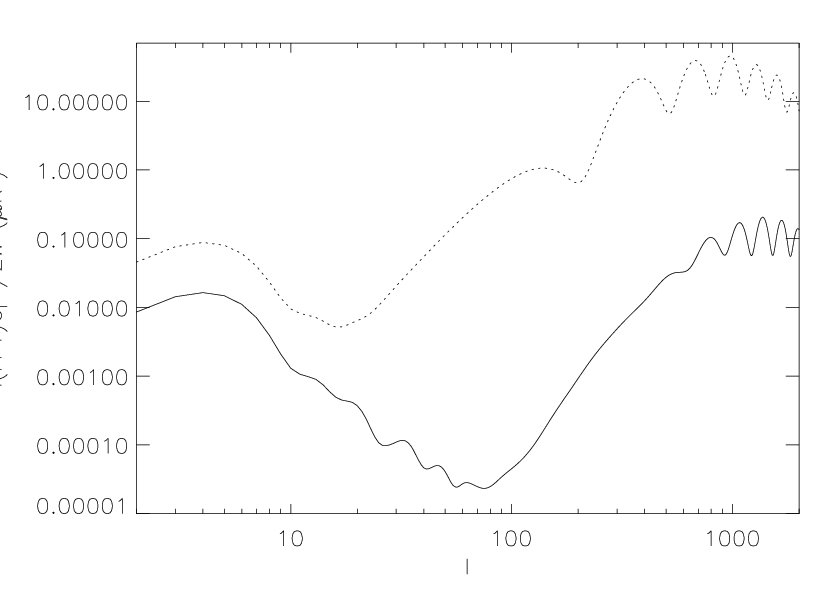
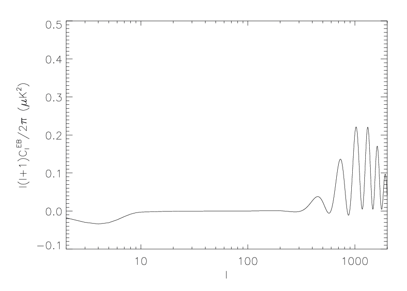
Figure 3: E​EE\,E (a), B​BB\,B (b), T​ET\,E (c), T​BT\,B (d), and E​BE\,B (e) angular power spectra for m=10−22m=10^{-22} eV and gϕ=10−20​eV−1g_{\phi}=10^{-20}\,\mbox{eV}^{-1} (black solid line), the black dotted line is the standard case in which there is no coupling between photons and pseudoscalars (θ=0\theta=0). For the B​BB\,B power spectrum (b) we plot for comparison also the polarization signal induced by gravitational lensing (black dotted line), and primordial B​BBB signal if r=0.1r=0.1 (blue dot-dashed line). The cosmological parameters of the flat Λ​C​D​M\Lambda CDM model used here are Ωb​h2=0.022\Omega_{b}\,h^{2}=0.022, Ωc​h2=0.123\Omega_{c}\,h^{2}=0.123, τ=0.09\tau=0.09, ns=1n_{s}=1, As=2.3×10⁻⁹A_{s}=2.3\times 10^{-9}, H0=100​h​km​s−1​Mpc−1=72​km​s−1​Mpc−1H_{0}=100\,h\,{\rm km\,s}^{-1}\,\mathrm{Mpc}^{-1}=72\,\mathrm{km\,s}^{-1}\,\mathrm{Mpc}^{-1}.

The linear polarization angle is not constant in time, but it oscillates with varying amplitude. If the field represents a fraction ΩMAT\Omega_{\mathrm{MAT}} of the universe energy density, then the amplitude of these oscillations is:

θA​(ΩMAT,m,gϕ)\displaystyle\theta_{A}(\Omega_{\mathrm{MAT}},m,g_{\phi}) =\displaystyle= 14​3​ΩMATπ​gϕ​Mpl​H0m​(1a03/2−1arec3/2)\displaystyle\frac{1}{4}\sqrt{\frac{3\Omega_{\mathrm{MAT}}}{\pi}}\frac{g_{\phi}M_{\mathrm{pl}}H_{0}}{m}\left(\frac{1}{a_{0}^{3/2}}-\frac{1}{a_{\mathrm{rec}}^{3/2}}\right) (90)
≃\displaystyle\simeq 14​3​ΩMATπ​gϕ​Mpl​H0m​zrec3/2.\displaystyle\frac{1}{4}\sqrt{\frac{3\Omega_{\mathrm{MAT}}}{\pi}}\frac{g_{\phi}M_{\mathrm{pl}}H_{0}}{m}z_{\mathrm{rec}}^{3/2}\,.

Fixed ΩMAT\Omega_{\mathrm{MAT}}, it is possible to constraint a certain region of the (m,gϕ)(m,g_{\phi})-plane requiring θA​(ΩMAT,m,gϕ)\theta_{A}(\Omega_{\mathrm{MAT}},m,g_{\phi}) to be smaller of a certain angle, typically of the order of few degrees (see Tab. 1). The excluded region considering current limits on CMB birefringence is shown in Fig. 2.

Fixed a particular value for the pseudoscalar field mass and for its coupling with photons we can also estimate how the polarization angular power spectra are modified by a rotation of the linear polarization plane. We modified the source term for linear polarization in the public Boltzmann code CAMB [31] following Eqs. (45) and (46). The linear polarization rotation angle is given by Eq. (88) and the evolution of the pseudoscalar field by Eq. (87). The new power spectra are compared with the standard unrotated ones in Fig. 3 fixed m=10−22m=10^{-22} eV and gϕ=10−20​eV−1g_{\phi}=10^{-20}\,\mbox{eV}^{-1}.

In Section VI we compare the power spectra modified version of CAMB obtained starting by Eqs. (45,46) which takes into account the time dependence of the pseudoscalar field in the integral along the line of sight with the approximated spectra obtained following Eqs. (55-59).

IV.3 Comments for axion cosmology

For axions the coupling constant with photons gϕg_{\phi} and the energy scale faf_{a} at which the new symmetry is broken are related [4]:

|gϕ|=αE​M2​π​fa​34​ξwith0.1≲ξ≲1,\left|g_{\phi}\right|=\frac{\alpha_{EM}}{2\pi f_{a}}\frac{3}{4}\xi\quad\mbox{with}\quad 0.1\lesssim\xi\lesssim 1\,, (91)

where the value for ξ\xi depends on the particular model considered for the axion. By using this relation a limit on the coupling constant is turned into a limit on the energy of symmetry breaking.

The critical density associated with the misalignment production of axions strongly depends on the initial misalignment angle associated with the axion field Θi\Theta_{i} through the following relation [3, 4]:

Ωm​i​s​h2∼0.23×10±0.6​(fa1012​GeV)1.175​Θi2​F​(Θi),\Omega_{mis}h^{2}\sim 0.23\times 10^{\pm 0.6}\left(\frac{f_{a}}{10^{12}\,\mbox{GeV}}\right)^{1.175}\Theta_{i}^{2}F\left(\Theta_{i}\right)\,, (92)

where hh encodes the actual value of the Hubble parameter (H0=100​h​km​s−1​Mpc−1H_{0}=100h\,\mbox{km}\,\mbox{s}^{-1}\,\mbox{Mpc}^{-1}) and F⁡(Θi)F(\Theta_{i}) accounts for anharmonic effects if Θi≫1\Theta_{i}\gg 1. The demand Ωm​i​s≤ΩD​M\Omega_{mis}\leq\Omega_{DM} provides an upper bound on fa1.175​Θi2f_{a}^{1.175}\Theta_{i}^{2} (assuming F⁡(Θi)≃1F\left(\Theta_{i}\right)\simeq 1) [26, 32, 33]:

fa​Θi1.7≤2×10¹¹÷12​GeV.f_{a}\Theta_{i}^{1.7}\leq 2\times 10^{11\div 12}\,\mbox{GeV}\,. (93)

This condition becomes also an upper bound for faf_{a} under the assumption that inflation occurred before the breaking of PQ-symmetry (fa≤fI​N​Ff_{a}\leq f_{INF}) [3]: in this scenario different regions have different values for Θi\Theta_{i}, so averaging over all observable universe the value of Θi\Theta_{i} in equation can replaced by its r​m​srms value (π/3\pi/\sqrt{3}) and the limit fa≤1011÷12​GeVf_{a}\leq 10^{11\div 12}\,\mbox{GeV} is obtained. As can be seen from Fig. 2, CAST disfavors values of gϕ∼10−11÷−12GeV−1g_{\phi}\sim 10^{-11\div-12}\,\mbox{GeV}^{-1} with a mass up to 0.02​eV0.02\mbox{eV}. Note however that our calculation cannot be applied directly to this case since we assume ϕ\phi homogeneous in our universe, whereas it is not if the PQ symmetry breaking occurs after inflation: although taking into account space inhomogeneities were a second order effect in cosmological perturbation theory, cosmological birefringence might be larger than the one computed in this paper.

Our calculations apply without modifications to the case in which inflation occurs after PQ-symmetry breaking: the initial misalignment angle Θi\Theta_{i} is homogeneous throughout our universe and can be much smaller than π/3\pi/\sqrt{3}. Such possibility allow the scale of PQ-symmetry breaking faf_{a} to be much higher than 1011÷12​GeV10^{11\div 12}\,\mbox{GeV} and is motivated by anthropic considerations [34, 35, 36, 37]. These smaller values of gϕg_{\phi} can be constrained by present data in CMB polarization in a much better way than CAST, in particular for small masses.

V Exponential potential

We consider in this section a pseudoscalar field with an exponential potential:

V⁡(ϕ)=V0​exp⁡(−λ​κ​ϕ),V\left(\phi\right)=V_{0}\exp\left(-\lambda\kappa\phi\right)\,, (94)

with κ2≡8​π​G.\kappa^{2}\equiv 8\pi G\,. Theoretical motivations to this kind of potential are certainly weaker than the ones for the potential presented in Eq. (60). However it is interesting to show how the kinematics of the pseudoscalar field is important for the resulting spectra of CMB anisotropies in polarization. Whereas the time derivative of the pseudoscalar field in the previous case contains oscillations about a vanishing value (see Eq. (69)), we study here a case where the behaviour is monotonous.

It is known [38] that exponential potential with λ2>3​(1+wF)\lambda^{2}>3(1+w_{\rm F}) leads to a component which tracks the dominant background fluid with equation of state pϕ=wϕ​ρϕp_{\phi}=w_{\phi}\rho_{\phi}. In order to satisfy the nucleosynthesis bound we choose λ=4.5\lambda=4.5. During the matter dominated era the scalar field behaves as:

ρϕ\displaystyle\rho_{\phi} =\displaystyle= ϕ˙22+V0​exp⁡(−λ​κ​ϕ)=f​ρMAT≡f​ρMAT,0a3,\displaystyle\frac{\dot{\phi}^{2}}{2}+V_{0}\exp\left(-\lambda\kappa\phi\right)=f\,\rho_{\rm MAT}\equiv f\frac{\rho_{\rm MAT,0}}{a^{3}}, (95)
Pϕ\displaystyle P_{\phi} =\displaystyle= ϕ˙22−V0​exp⁡(−λ​κ​ϕ),\displaystyle\frac{\dot{\phi}^{2}}{2}-V_{0}\exp\left(-\lambda\kappa\phi\right), (96)

where ρMAT=ρDM+ρbaryons+ρϕ\rho_{\rm MAT}=\rho_{\rm DM}+\rho_{\rm baryons}+\rho_{\phi}.

For λ=4.5\lambda=4.5 the contribution of the pseudoscalar field to universe energy density is shown in Fig. 4. The value of Ωϕ\Omega_{\phi} changes with time, but it is almost constant (Ωϕ≃Ωϕ,0=0.148\Omega_{\phi}\simeq\Omega_{\phi\,,0}=0.148) from recombination (log⁡arec≃−7\log a_{\rm rec}\simeq-7) to nowadays.

Refer to caption
Figure 4: For λ=4.5\lambda=4.5 Dashed line: ΩDM+Ωbaryons\Omega_{\rm DM}+\Omega_{\rm baryons}, dotted line: ΩRAD\Omega_{\rm RAD}, thin continuous line: Ωϕ\Omega_{\rm\phi}, thick continuous line: wϕw_{\rm\phi}, in terms of the natural logarithm of the scale factor (from log⁡a≃−40\log a\simeq-40 to nowadays log⁡a0=0\log a_{0}=0). Here ΩDM,0+Ωbaryons,0=0.852\Omega_{\rm DM,0}+\Omega_{\rm baryons,0}=0.852 and Ωϕ,0=0.148\Omega_{\rm\phi,0}=0.148.

The derivative of the pseudoscalar field respect to conformal time is proportional to a−1/2a^{-1/2} and the evolution of the scale factor in the matter dominated phase is a⁡(η)=(η/η0)2a(\eta)=(\eta/\eta_{0})^{2} so:

ϕ′=f​ρMAT,0​η0η.\phi^{\prime}=\sqrt{f\,\rho_{\rm MAT,0}}\frac{\eta_{0}}{\eta}\,. (97)

Substituting this relation in Eq. (14) we obtain the following expression for the evolution of the electromagnetic potential:

A~±′′+(k2±gϕ​f​ρMAT,0​η0η​k)​A~±=0.\tilde{A}_{\pm}^{\prime\prime}+\left(k^{2}\pm g_{\phi}\sqrt{f\,\rho_{\rm MAT,0}}\frac{\eta_{0}}{\eta}k\right)\tilde{A}_{\pm}=0\,. (98)

This is a particular differential equation, called Coulomb wave equation; defining q±≡∓gϕf​ρMAT,0η0/2=∓qq_{\pm}\equiv\mp g_{\phi}\sqrt{f\,\rho_{\rm MAT,0}}\eta_{0}/2=\mp q and x≡k​ηx\equiv k\eta it becomes:

d2​A~±d​x2+(1−2​q±x)​A~±=0.\frac{d^{2}\tilde{A}_{\pm}}{dx^{2}}+\left(1-\frac{2q_{\pm}}{x}\right)\tilde{A}_{\pm}=0\,. (99)

The solution of this particular equation can be written in terms of regular (F0​(q,x)F_{0}(q,x)) and irregular (G0​(q,x)G_{0}(q,x)) Coulomb wave functions [39, 40]:

A~+\displaystyle\tilde{A}_{+} =\displaystyle= f+​F0​(q+,x)+g+​G0​(q+,x)\displaystyle f_{+}F_{0}(q_{+},x)+g_{+}G_{0}(q_{+},x)
=\displaystyle= f+​F0​(−q,x)+g+​G0​(−q,x),\displaystyle f_{+}F_{0}(-q,x)+g_{+}G_{0}(-q,x)\,,
A~−\displaystyle\tilde{A}_{-} =\displaystyle= f−​F0​(q−,x)+g−​G0​(q−,x)\displaystyle f_{-}F_{0}(q_{-},x)+g_{-}G_{0}(q_{-},x)
=\displaystyle= f−​F0​(q,x)+g−​G0​(q,x),\displaystyle f_{-}F_{0}(q,x)+g_{-}G_{0}(q,x)\,,

where f+,f−,g+,g−∈ℂf_{+},f_{-},g_{+},g_{-}\in\mathbb{C}; in a compact notation:

A~±​(q,x)\displaystyle\tilde{A}_{\pm}(q,x) =\displaystyle= f±​F0​(∓q,x)+g±​G0​(∓q,x).\displaystyle f_{\pm}F_{0}(\mp q,x)+g_{\pm}G_{0}(\mp q,x)\,. (100)

The Stokes parameters contain the derivative respect to conformal time η\eta, so we evaluate:

A~±′​(q,x)\displaystyle\tilde{A}_{\pm}^{\prime}(q,x) =\displaystyle= k⁡[f±​∂F0​(∓q,x)∂x+g±​∂G0​(∓q,x)∂x].\displaystyle k\left[f_{\pm}\frac{\partial F_{0}(\mp q,x)}{\partial x}+g_{\pm}\frac{\partial G_{0}(\mp q,x)}{\partial\,x}\right]\,. (101)

The solution given in Eq. (100) verifies the Wronskian condition (A~±​A~±′⁣∗−A~±′​A~±∗=i\tilde{A}_{\pm}\tilde{A}_{\pm}^{\prime*}-\tilde{A}_{\pm}^{\prime}\tilde{A}_{\pm}^{*}=i) if the following relation holds:

f±∗​g±−f±​g±∗=ik⟹ℑ⁡(f±∗​g±)=12​k.f_{\pm}^{*}g_{\pm}-f_{\pm}g_{\pm}^{*}=\frac{i}{k}\quad\Longrightarrow\quad\Im\left(f_{\pm}^{*}g_{\pm}\right)=\frac{1}{2k}\,. (102)

In the general case, when the coupling does not vanishes (gϕ≠0g_{\phi}\neq 0), we expand the solution (100) for large value of xx neglecting terms proportional to 𝒪⁡(x−2)\mathcal{O}(x^{-2}) (see Appendix):

A~±​(q,x)\displaystyle\tilde{A}_{\pm}(q,x) ≃\displaystyle\simeq f±​[q22​x​cos⁡(x±α⁡(q,x))+(1∓q2​x)​sin⁡(x±α⁡(q,x))]\displaystyle f_{\pm}\left[\frac{q^{2}}{2x}\cos\left(x\pm\alpha\left(q,x\right)\right)+\left(1\mp\frac{q}{2x}\right)\sin\left(x\pm\alpha\left(q,x\right)\right)\right] (103)
+g±​[(1∓q2​x)​cos⁡(x±α⁡(q,x))−q22​x​sin⁡(x±α⁡(q,x))],\displaystyle+g_{\pm}\left[\left(1\mp\frac{q}{2x}\right)\cos\left(x\pm\alpha\left(q,x\right)\right)-\frac{q^{2}}{2x}\sin\left(x\pm\alpha\left(q,x\right)\right)\right]\,,

where α⁡(q,x)≡q​ln⁡2​x−arg⁡Γ⁡(1+i​q)\alpha\left(q,x\right)\equiv q\ln 2x-\arg\Gamma(1+iq). The derivative respect to conformal time is:

A~±′​(q,x)\displaystyle\tilde{A}_{\pm}^{\prime}(q,x) ≃\displaystyle\simeq k{f±[(1±q2​x)cos(x±α(q,x))−q22​xsin(x±α(q,x))]\displaystyle k\left\{f_{\pm}\left[\left(1\pm\frac{q}{2x}\right)\cos\left(x\pm\alpha\left(q,x\right)\right)-\frac{q^{2}}{2x}\sin\left(x\pm\alpha\left(q,x\right)\right)\right]\right. (104)
+g±[−q22​xcos(x±α(q,x))−(1±q2​x)sin(x±α(q,x))]}\displaystyle\left.+g_{\pm}\left[-\frac{q^{2}}{2x}\cos\left(x\pm\alpha\left(q,x\right)\right)-\left(1\pm\frac{q}{2x}\right)\sin\left(x\pm\alpha\left(q,x\right)\right)\right]\right\}
=k2[ei⁡(x±α⁡(q,x))(1±q2​x+iq22​x)(f±+ig±)\displaystyle=\frac{k}{2}\left[e^{i\left(x\pm\alpha\left(q,x\right)\right)}\left(1\pm\frac{q}{2x}+i\frac{q^{2}}{2x}\right)\left(f_{\pm}+ig_{\pm}\right)\right.
e−i⁡(x±α⁡(q,x))(1±q2​x−iq22​x)(f±−ig±)].\displaystyle\left.e^{-i\left(x\pm\alpha\left(q,x\right)\right)}\left(1\pm\frac{q}{2x}-i\frac{q^{2}}{2x}\right)\left(f_{\pm}-ig_{\pm}\right)\right]\,.

In general both forward moving waves (A~±∝e−i​k​η\tilde{A}_{\pm}\propto e^{-ik\eta}) and backward moving waves (A~±∝ei​k​η\tilde{A}_{\pm}\propto e^{ik\eta}) must be taken into account for propagation of light in a medium. Chosen a particular value for the constants f±f_{\pm} and g±g_{\pm} that verifies the Wronskian relation (102) the evolution of polarization is fixed.

If we assume, according with [41, 42], that the photon pseudoscalar conversion is a small effect due to low energy of CMB photons, the production of backward moving waves can be neglected (see [43] for the use of this approximation). The Eq. (104) setting f±=−i​g±f_{\pm}=-ig_{\pm} becomes:

A~±′​(q,x)≃−i​k​g±​(1±q2​x−i​q22​x)​e−i⁡(x±α⁡(q,x)),\tilde{A}^{\prime}_{\pm}\left(q,x\right)\simeq-ikg_{\pm}\left(1\pm\frac{q}{2x}-i\frac{q^{2}}{2x}\right)e^{-i\left(x\pm\alpha(q,x)\right)}\,, (105)

and in terms of the value at recombination time:

A~±′(q,x)≃A~±′(q,xrec)[1±q2(1x−1xrec)\displaystyle\tilde{A}^{\prime}_{\pm}\left(q,x\right)\simeq\tilde{A}^{\prime}_{\pm}\left(q,x_{\rm rec}\right)\left[1\pm\frac{q}{2}\left(\frac{1}{x}-\frac{1}{x_{\rm rec}}\right)\right.
−iq22(1x−1xrec)]exp{−i[x−xrec±Δα]},\displaystyle\left.-i\frac{q^{2}}{2}\left(\frac{1}{x}-\frac{1}{x_{\rm rec}}\right)\right]\exp\left\{-i\left[x-x_{\rm rec}\pm\Delta\alpha\right]\right\}\,, (106)

where we have introduced

Δ​α\displaystyle\Delta\alpha ≡\displaystyle\equiv α⁡(q,x)−α⁡(q,xrec)=q​ln⁡(η/ηrec)\displaystyle\alpha(q,x)-\alpha(q,x_{\rm rec})=q\ln\left(\eta/\eta_{\rm rec}\right) (107)
=\displaystyle= q2​ln⁡(a/arec).\displaystyle\frac{q}{2}\ln\left(a/a_{\rm rec}\right)\,.

We observe that also in this exact case the plane of linear polarization is rotated of an angle Δ​α\Delta\alpha independent on kk whose dependence on the difference between the present value of ϕ\phi and the corresponding one at recombination is the same of the adiabatic approximation and of Eq. (59).

Refer to caption Refer to caption
Refer to caption
Figure 5: E​EE\,E (a), B​BB\,B (b), T​ET\,E (c), T​BT\,B (d) and E​BE\,B (e) angular power spectra for gϕ=10−28​eV−1g_{\phi}=10^{-28}\,\mbox{eV}^{-1} (black solid line); the black dotted line is the standard case in which there is no coupling (θ=0\theta=0). For the B​BB\,B power spectrum (b) we plot for comparison also the polarization signal induced by gravitational lensing (black dotted line), and primordial B​BBB signal if r=0.1r=0.1 (blue dot-dashed line). The cosmological parameters of the flat C​D​MCDM model used here are Ωb=0.0462\Omega_{b}=0.0462, Ωc=0.9538\Omega_{c}=0.9538 (Ωϕ≃0.148\Omega_{\phi}\simeq 0.148), τ=0.09\tau=0.09, ns=1n_{s}=1, As=2.3×10⁻⁹A_{s}=2.3\times 10^{-9}, H0=72​km​s−1​Mpc−1H_{0}=72\,\mathrm{km\,s}^{-1}\,\mathrm{Mpc}^{-1}.

Current measures and constraints on the polarization pattern of CMB anisotropies produce an upper limit on the linear polarization rotation angle of the order of few degrees (see Tab. 1). We now use these constraints and our analytic expression:

|θ|\displaystyle\left|\theta\right| =\displaystyle= |q|2​ln⁡(1+zrec)\displaystyle\frac{|q|}{2}\ln(1+z_{\mathrm{rec}}) (108)
≃\displaystyle\simeq 14​32​π​Ωϕ,0​|gϕ|​Mpl​ln⁡(1+zrec),\displaystyle\frac{1}{4}\sqrt{\frac{3}{2\pi}\Omega_{\phi,0}}\left|g_{\phi}\right|M_{\mathrm{pl}}\ln(1+z_{\mathrm{rec}})\,,

to obtain an upper bound for qq, which can be turned into a upper bound on gϕg_{\phi}; if |θ|≲6\left|\theta\right|\lesssim 6 deg, then:

|gϕ|≲10−30​eV−1,\left|g_{\phi}\right|\lesssim 10^{-30}\,\mbox{eV}^{-1}\,, (109)

where we have assumed: Ωϕ,0≃0.148\Omega_{\phi,0}\simeq 0.148 and zrec≃1100z_{\mathrm{rec}}\simeq 1100.

The angle of linear polarization θ⁡(η)\theta(\eta) appearing in Eqs. (45) and (46) can be replaced with:

|θ⁡(η)|≃12​32​π​Ωϕ,0​|gϕ|​Mpl​ln⁡(ηηrec),\left|\theta(\eta)\right|\simeq\frac{1}{2}\sqrt{\frac{3}{2\pi}\Omega_{\phi,0}}\left|g_{\phi}\right|M_{\mathrm{pl}}\ln\left(\frac{\eta}{\eta_{\mathrm{rec}}}\right)\,, (110)

and the polarization power spectra are evaluated using the expression given in Section III.2, see angular power spectra of Fig. 5.

In Section VI we compare the power spectra modified version of CAMB obtained starting by Eqs. (45,46) which takes into account the time dependence of the pseudoscalar field in the integral along the line of sight with the approximated spectra obtained following Eqs. (55-60).

VI Comparison with constant rotation angle approximation
Refer to caption Refer to caption
Refer to caption
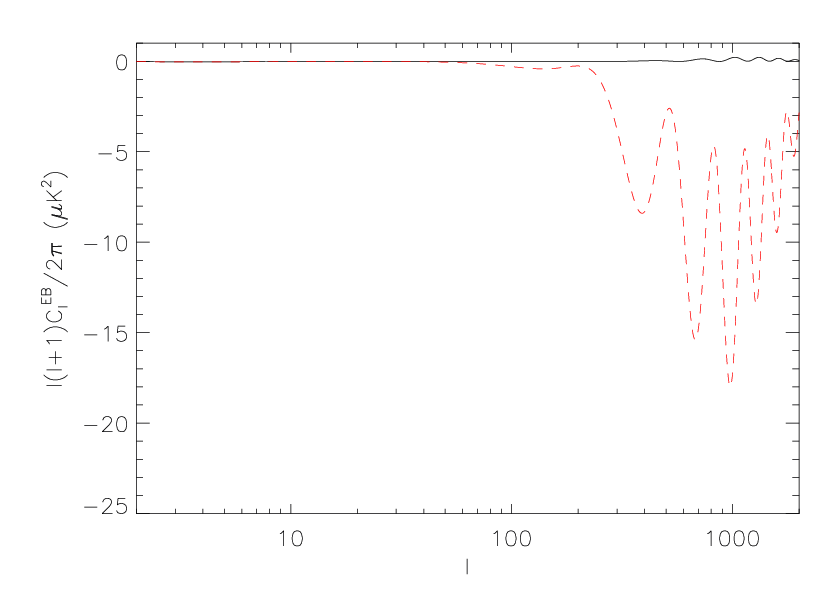
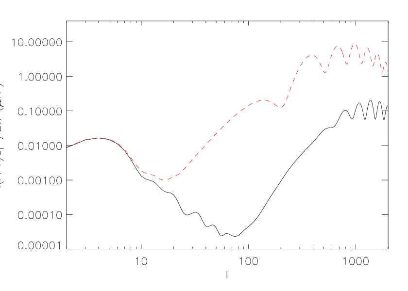
Figure 6: E​EE\,E (a), B​BB\,B (b), T​ET\,E (c), T​BT\,B (d) and E​BE\,B (e) angular power spectra for m=10−22m=10^{-22} eV and gϕ=10−20​eV−1g_{\phi}=10^{-20}\,\mbox{eV}^{-1} (black solid line) and approximating the rotation angle with the constant value θrec\theta_{\mathrm{rec}} (red dashed line). The cosmological parameters of the flat Λ​C​D​M\Lambda CDM model used here are Ωb​h2=0.022\Omega_{b}\,h^{2}=0.022, Ωc​h2=0.123\Omega_{c}\,h^{2}=0.123, τ=0.09\tau=0.09, ns=1n_{s}=1, As=2.3×10⁻⁹A_{s}=2.3\times 10^{-9}, H0=100​h​km​s−1​Mpc−1=72​km​s−1​Mpc−1H_{0}=100\,h\,{\rm km\,s}^{-1}\,\mathrm{Mpc}^{-1}=72\,\mathrm{km\,s}^{-1}\,\mathrm{Mpc}^{-1}.
Refer to caption Refer to caption
Refer to caption
Figure 7: E​EE\,E (a), B​BB\,B (b), T​ET\,E (c), T​BT\,B (d) and E​BE\,B (e) angular power spectra for gϕ=10−28​eV−1g_{\phi}=10^{-28}\,\mbox{eV}^{-1} (black solid line) and approximating the rotation angle with the constant value θrec\theta_{\mathrm{rec}} (red dashed line); the black dotted line is the standard case in which there is no coupling. The cosmological parameters of the flat C​D​MCDM model used here are Ωb=0.0462\Omega_{b}=0.0462, Ωc=0.9538\Omega_{c}=0.9538 (Ωϕ≃0.148\Omega_{\phi}\simeq 0.148), τ=0.09\tau=0.09, ns=1n_{s}=1, As=2.3×10⁻⁹A_{s}=2.3\times 10^{-9}, H0=72​km​s−1​Mpc−1H_{0}=72\,\mathrm{km\,s}^{-1}\,\mathrm{Mpc}^{-1}.

In this section we compare the angular power spectra obtained modifying the public code CAMB [31] considering the correct dynamic of the pseudoscalar field (θ=θ⁡(η)\theta=\theta(\eta)) as described in Section III.2, with the ones obtained in the constant rotation angle approximation (θ=const\theta=\mbox{const}) for the two different potential considered in the previous sections: see Figs. 6 and 7.

In Section III.2 we have already shown how the power spectra in the constant rotation angle approximation [Eqs. (54)-(58)] can be obtained from the general expressions [Eqs. (47)-(51)].

Power spectrum modifications obtained starting directly form the Boltzmann equations and taking into account the temporal evolution of the pseudoscalar field are usually smaller than effects predicted considering a constant rotation angle equal to the total rotation angle from last scattering to nowadays. If the cosmological pseudoscalar field evolves quickly, then the constant rotation angle approximation clearly leads to an overestimate of the effects.

It is important to stress that the constant rotation angle approximation is just an operative approximation. The additional term in the Boltzmann equations which rotates the linear polarization plane is (see Eq. 38):

∓i​2​θ′​(η)​ΔQ±i​U​(k,η),\mp i2\theta^{\prime}(\eta)\Delta_{Q\pm iU}(k,\eta)\,, (111)

which clearly vanishes for θ=const\theta=\mbox{const}.

VII Conclusions

We have studied the impact of a pseudoscalar field acting as dark matter on CMBP. We have shown that such pseudoscalar interaction with photons rotates the plane of linear polarization and generates circular polarization. In absence of measures for the VV mode of CMBP, the existing upper limits on an isotropic T​BT\,B and E​BE\,B correlations can constrain the coupling constants of photons with the pseudoscalar field.

We have examined two representative examples for the dynamics of a pseudo-Goldstone field behaving as dark matter: the oscillating and the monotonic decreasing behavior. In the monotonic decreasing behavior, by neglecting backward moving waves, we have shown how present CMB observations can constrain the coupling constant gϕg_{\phi} to small values as 𝒪⁡(10−30)\mathcal{O}\left(10^{-30}\right) eV. For the more physically motivated axion case which leads to an oscillating behaviour, we have shown how constraints from CMB cosmological birefringence can become important for small masses for the axion.

We have also shown how the use of integral solution of the Boltzmann function may improve the estimate obtained by multiplying the CMB power spectrum by the suitable trigonometric functions of the rotation angle as in Eqs. (54-58).

Acknowledgements

We wish to thank Daniela Paoletti, Günter Sigl and Guido Zavattini for discussions. FF and MG are partially supported by INFN IS PD51 and by the ASI contract ‘Planck LFI Activity of Phase E2’. FF is partially supported by INFN IS BO11.

Coulomb wave equation

The Coulomb wave equation is [39]:

d2​wd​x2−[1−2​qx−L⁡(L+1)x2]​w=0,\frac{d^{2}w}{dx^{2}}-\left[1-\frac{2q}{x}-\frac{L(L+1)}{x^{2}}\right]w=0\,, (112)

with x>0,−∞<q<∞,Lx>0,-\infty<q<\infty,L a non negative integer. Here, in order to solve Eq. (99), we are particular interested to the particular case when L=0.

The solution can be written in terms of regular (FL​(q,x)F_{L}(q,x)) and irregular (GL​(q,x)G_{L}(q,x)) Coulomb wave function:

w=c1​FL​(q,x)+c2​GL​(q,x).w=c_{1}F_{L}(q,x)+c_{2}G_{L}(q,x)\,. (113)

The Coulomb functions can be expanded for large values of xx [39]:

F0\displaystyle F_{0} =\displaystyle= g​cos⁡θ+f​sin⁡θ,\displaystyle g\cos\theta+f\sin\theta\,, (114)
G0\displaystyle G_{0} =\displaystyle= f​cos⁡θ−g​sin⁡θ,\displaystyle f\cos\theta-g\sin\theta\,, (115)

similarly for the first derivative respect to xx

F0′\displaystyle F_{0}^{\prime} =\displaystyle= g∗​cos⁡θ+f∗​sin⁡θ,\displaystyle g^{*}\cos\theta+f^{*}\sin\theta\,, (116)
G0′\displaystyle G_{0}^{\prime} =\displaystyle= f∗​cos⁡θ−g∗​sin⁡θ,\displaystyle f^{*}\cos\theta-g^{*}\sin\theta\,, (117)

with θ≡x−q​ln⁡2​x+arg⁡Γ⁡(1+i​q)\theta\equiv x-q\ln 2x+\arg\Gamma(1+iq) and:

f=∑k=0∞fk,\displaystyle f=\sum_{k=0}^{\infty}f_{k}\,, g=∑k=0∞gk,\displaystyle g=\sum_{k=0}^{\infty}g_{k}\,,
f∗=∑k=0∞fk∗,\displaystyle\quad f^{*}=\sum_{k=0}^{\infty}f^{*}_{k}\,, g∗=∑k=0∞gk∗,\displaystyle g^{*}=\sum_{k=0}^{\infty}g^{*}_{k}\,,

where:

f0=1,fk+1=ak​fk−bk​gk;\displaystyle f_{0}=1\,,\quad f_{k+1}=a_{k}f_{k}-b_{k}g_{k}\,; (118)
g0=0,gk+1=ak​gk+bk​fk;\displaystyle g_{0}=0\,,\quad g_{k+1}=a_{k}g_{k}+b_{k}f_{k}\,; (119)
f0∗=0,fk+1∗=ak​fk∗−bk​gk∗−fk+1x;\displaystyle f_{0}^{*}=0\,,\quad f_{k+1}^{*}=a_{k}f_{k}^{*}-b_{k}g_{k}^{*}-\frac{f_{k+1}}{x}\,; (120)
g0∗=1−qx,gk+1∗=ak​gk∗+bk​fk∗−gk+1x;\displaystyle g_{0}^{*}=1-\frac{q}{x}\,,\quad g_{k+1}^{*}=a_{k}g_{k}^{*}+b_{k}f_{k}^{*}-\frac{g_{k+1}}{x}\,; (121)
ak=(2​k+1)​q2​(k+1)​x,bk=q2−k⁡(k+1)2​(k+1)​x.\displaystyle a_{k}=\frac{(2k+1)q}{2(k+1)x}\,,\quad b_{k}=\frac{q^{2}-k(k+1)}{2(k+1)x}\,. (122)

Restricting to the first order:

f=1+q2​x+𝒪⁡(1x2),\displaystyle f=1+\frac{q}{2x}+\mathcal{O}\left(\frac{1}{x^{2}}\right)\,, (123)
g=q22​x+𝒪⁡(1x2),\displaystyle g=\frac{q^{2}}{2x}+\mathcal{O}\left(\frac{1}{x^{2}}\right)\,, (124)
f∗=−q22​x+𝒪⁡(1x2),\displaystyle f^{*}=-\frac{q^{2}}{2x}+\mathcal{O}\left(\frac{1}{x^{2}}\right)\,, (125)
g∗=1−q2​x+𝒪⁡(1x2).\displaystyle g^{*}=1-\frac{q}{2x}+\mathcal{O}\left(\frac{1}{x^{2}}\right)\,. (126)

Summarizing the asymptotic expansion of FL​(q,x)F_{L}(q,x) and FL​(q,x)F_{L}(q,x) for large values of xx is:

F0​(q,x)≃q22​x​cos⁡θ+(1+q2​x)​sin⁡θ,\displaystyle F_{0}(q,x)\simeq\frac{q^{2}}{2x}\cos\theta+\left(1+\frac{q}{2x}\right)\sin\theta\,, (127)
G0​(q,x)≃(1+q2​x)​cos⁡θ−q22​x​sin⁡θ,\displaystyle G_{0}(q,x)\simeq\left(1+\frac{q}{2x}\right)\cos\theta-\frac{q^{2}}{2x}\sin\theta\,, (128)

and for the first derivative:

F0′​(q,x)≃(1−q2​x)​cos⁡θ−q22​x​sin⁡θ,\displaystyle F_{0}^{\prime}(q,x)\simeq\left(1-\frac{q}{2x}\right)\cos\theta-\frac{q^{2}}{2x}\sin\theta\,, (129)
G0′​(q,x)≃−q22​x​cos⁡θ−(1−q2​x)​sin⁡θ.\displaystyle G_{0}^{\prime}(q,x)\simeq-\frac{q^{2}}{2x}\cos\theta-\left(1-\frac{q}{2x}\right)\sin\theta\,. (130)

References

  • [1] R. D. Peccei and H. R. Quinn, Phys. Rev. Lett. 38 (1977) 1440.
  • [2] J. E. Kim, Phys. Rept. 150 (1987) 1.
  • [3] E. W. Kolb and M. S. Turner, “The Early universe,” Front. Phys. 69 (1990) 1.
  • [4] G. G. Raffelt, “Stars As Laboratories For Fundamental Physics: The Astrophysics Of Neutrinos, Axions, And Other Weakly Interacting Particles,”, 1996 Chicago, USA: Univ. Pr.
  • [5] P. Sikivie, Lect. Notes Phys. 741, 19 (2008) [arXiv:astro-ph/0610440].
  • [6] S. Andriamonje et al. [CAST Collaboration], JCAP 0704 (2007) 010 [arXiv:hep-ex/0702006].
  • [7] G. G. Raffelt, Lect. Notes Phys. 741, 51 (2008) [arXiv:hep-ph/0611350].
  • [8] D. Harari and P. Sikivie, Phys. Lett. B 289 (1992) 67.
  • [9] S. M. Carroll and G. B. Field, Phys. Rev. D 43 (1991) 3789.
  • [10] S. M. Carroll and G. B. Field, Phys. Rev. Lett. 79 (1997) 2394 [arXiv:astro-ph/9704263].
  • [11] A. Lue, L. M. Wang and M. Kamionkowski, Phys. Rev. Lett. 83 (1999) 1506 [arXiv:astro-ph/9812088].
  • [12] M. Zaldarriaga and U. Seljak, Phys. Rev. D 55 (1997) 1830 [arXiv:astro-ph/9609170].
  • [13] M. Zaldarriaga, arXiv:astro-ph/9806122.
  • [14] W. Hu and M. J. White, New Astron. 2 (1997) 323 [arXiv:astro-ph/9706147].
  • [15] B. Feng, M. Li, J. Q. Xia, X. Chen and X. Zhang, Phys. Rev. Lett. 96 (2006) 221302 [arXiv:astro-ph/0601095].
  • [16] P. Cabella, P. Natoli and J. Silk, Phys. Rev. D 76, 123014 (2007) [arXiv:0705.0810 [astro-ph]].
  • [17] E. Komatsu et al. [WMAP Collaboration], arXiv:0803.0547 [astro-ph].
  • [18] G. C. Liu, S. Lee and K. W. Ng, Phys. Rev. Lett. 97, 161303 (2006) [arXiv:astro-ph/0606248].
  • [19] K. R. S. Balaji, R. H. Brandenberger and D. A. Easson, JCAP 0312, 008 (2003) [arXiv:hep-ph/0310368].
  • [20] W. D. Garretson, G. B. Field and S. M. Carroll, Phys. Rev. D 46 (1992) 5346 [arXiv:hep-ph/9209238].
  • [21] F. Finelli and A. Gruppuso, Phys. Lett. B 502, 216 (2001) [arXiv:hep-ph/0001231].
  • [22] C. W. Misner, K. S. Thorne and J. A. Wheeler, “Gravitation,”,1973 San Francisco
  • [23] A. Kosowsky, Annals Phys. 246 (1996) 49 [arXiv:astro-ph/9501045].
  • [24] G. C. Liu, N. Sugiyama, A. J. Benson, C. G. Lacey and A. Nusser, Astrophys. J. 561, 504 (2001) [arXiv:astro-ph/0101368].
  • [25] E. Y. Wu et al. [QUaD Collaboration], arXiv:0811.0618 [astro-ph].
  • [26] M. Dine and W. Fischler, Phys. Lett. B 120, 137 (1983).
  • [27] M. S. Turner, Phys. Rev. D 28, 1243 (1983).
  • [28] Note that if we had included k2​(|A~+′|2−|A~−′|2)k^{2}(|\tilde{A}_{+}^{\prime}|^{2}-|\tilde{A}_{-}^{\prime}|^{2}) in the definition of VV in Eq. (34), the ratio in Eq. (81) would be proportional to 𝒪⁡(k−3){\cal O}(k^{-3}).
  • [29] D. S. Lee and K. W. Ng, Phys. Rev. D 61, 085003 (2000) [arXiv:hep-ph/9909282].
  • [30] A. Gruppuso and F. Finelli, Phys. Rev. D 73, 023512 (2006) [arXiv:astro-ph/0512641].
  • [31] A. Lewis, A. Challinor and A. Lasenby, Astrophys. J. 538, 473 (2000) [arXiv:astro-ph/9911177].
  • [32] L. F. Abbott and P. Sikivie, Phys. Lett. B 120, 133 (1983).
  • [33] J. Preskill, M. B. Wise and F. Wilczek, Phys. Lett. B 120, 127 (1983).
  • [34] S. Y. Pi, Phys. Rev. Lett. 52, 1725 (1984).
  • [35] A. D. Linde, Phys. Lett. B 201, 437 (1988).
  • [36] M. Tegmark, A. Aguirre, M. Rees and F. Wilczek, Phys. Rev. D 73, 023505 (2006) [arXiv:astro-ph/0511774].
  • [37] M. P. Hertzberg, M. Tegmark and F. Wilczek, arXiv:0807.1726 [astro-ph].
  • [38] E. J. Copeland, A. R. Liddle and D. Wands, Phys. Rev. D 57, 4686 (1998) [arXiv:gr-qc/9711068].
  • [39] M. Abramowitz and I. A. Stegun, “Handbook of Mathematical Functions with Formulas, Graphs, and Mathematical Tables”, (Dover, New York, USA, 1964).
  • [40] M. M. Anber and L. Sorbo, JCAP 0610 (2006) 018 [arXiv:astro-ph/0606534].
  • [41] P. Jain, S. Panda and S. Sarala, Phys. Rev. D 66 (2002) 085007 [arXiv:hep-ph/0206046].
  • [42] A. Mirizzi, G. G. Raffelt and P. D. Serpico, Lect. Notes Phys. 741, 115 (2008) [arXiv:astro-ph/0607415].
  • [43] S. Das, P. Jain, J. P. Ralston and R. Saha, JCAP 0506 (2005) 002 [arXiv:hep-ph/0408198].