Study of the top reconstruction in top-partner events at the LHC
Abstract
In the Littlest Higgs model with T-parity (LHT), top-partners () are produced in pairs at the Large Hadron Collider (LHC). Each top-partner decays into a top quark () and the lightest -odd gauge partner . We demonstrate reconstruction of the system decaying hadronically, and measurement of the top-partner mass from the distribution. A top quark from a decay is polarized, and we discuss the effect of this polarization on the decay distributions. Because the events consist of highly collinear jets which occasionally overlap each other, we compare distributions using different jet reconstruction algorithms (Snowmass cone, kt, Cambridge, SISCone). We find clustering algorithms are advantageous for studying top polarization effects.
I Introduction
In spite of the success of the Standard Model (SM) in explaining the particle interactions, there are yet two unsolved questions in the SM. One is the fine tuning problem and the other is the existence of the dark matter (DM) in our universe.
The fine tuning problem is the question why the Higgs is likely to be so light as expected from the LEP data ( at the 95% confidence level [1]), while naturally the Higgs mass is the order of the cut off scale of the theory due to radiative corrections. Some mechanism should protect the Higgs mass, and interactions involving the Higgs sector should be extended from the SM one.
The existence of the DM is now established by the cosmological observations such as WMAP, SDSS and SN-Ia [2, 3, 4, 5, 6]. The SM should be extended to include the DM, which should be a neutral stable particle. Moreover, provided that the DM is a thermal relic whose strength of the coupling to the SM particles of the order of the weak interaction, the mass can be a few 100 GeV from a rough dimensional analysis.
To solve the fine tuning problem, many models have been proposed. However, a so-called “little hierarchy problem” [7, 8] arises in these models, once constraints from precision measurements are imposed. New operators arising from these models naively have the cut off scale TeV to be consistent to the experimental data [9].
Some successful models solving the little hierarchy problem have parity structures, for example the MSSM with R-parity [10, 11, 12], the little Higgs model with T-parity (LHT) [16, 17, 13, 14, 15], or the universal extra dimensional model (UED) with KK-parity [18, 19]. Such a model which has a parity structure predicts the stable lightest parity odd particle as a candidate of the DM. The cut off scale of new operators in the model can be as low as a few TeV [20], and the mass of the lightest parity odd particle can be on the order of a few 100 GeV.
The LHC is starting soon, and it is likely to discover new particles with masses up to a few TeV [21, 22]. The models mentioned above are studied intensively by many authors. All of these models have partners of the SM colored particles which decay into the stable lightest parity odd particle through the parity conserving interactions.
At the LHC, these partners are produced in pairs. The signal is multiple high jets and high leptons, each accompanied by missing transverse momentum . Among the signals studied so far, the signals with high leptons are very promising [23, 24], because the SM backgrounds are smaller. However, branching ratios of new particles into leptons strongly depend on model parameters. In addition, Jets + leptons signals are often accompanied by undetectable neutrinos, which are also the source of missing momentum. They sometimes reduce the significance of the kinematical endpoints of the signal distributions for mass reconstructions. And even in the case that the lepton branching ratios are small, events with multiple jets and no lepton are enormously produced.
In this paper, we focus on the top partner signal in the LHT. The top partner pair productions occur with sizable cross section [25] compared with stop pair productions in the MSSM because the top partner is a fermion. The event has simple kinematics, where top quarks are highly boosted11 1 Similar highly boosted signals have been discussed in the RS1 model [26]. However, it is different from the signal considered in this paper, because it is not accompanied by .. Decay products from a boosted top are collimated and they are easily identified as a jet system with mass with high probability using hemisphere analysis [27, 28]. On the other hand, by imposing lepton veto and top tagging, background events from jets can be reduced significantly.
The process above was partly studied in Ref. [28]. In the paper, COMPHEP [29] and HERWIG6.5 [30] are used for the event generation and AcerDET1.0 [32] is used for the detector simulation and jet reconstruction. AcerDET1.0 implements the Snowmass cone algorithm. However, the algorithm is not optimized in resolving the overlapping jets arising from boosted top quark correctly.
Recently, FastJet [33] was released. Infrared stable jet reconstruction algorithms (kt [34, 35, 36, 37], Cambridge [38, 39], SISCone [40]) are implemented in the code, which is significantly faster than previous codes. We study improvements with these advanced jet reconstruction algorithms. In this study, we interface AcerDET calorimeter information to FastJet and reanalyze the same process as in Ref. [28] to compare the results. We find the kt and Cambridge algorithm have advantage to resolve overlapping jets. We also generate the signal events with underlying events using HERWIG6.5 + Jimmy [41], and find the jet resolution with the kt algorithm is significantly affected by underlying events. This motivates us to show results with the Cambridge algorithm mainly in this paper.
We study the potential to measure the mass of the top partner using the reconstructed top candidates, although only the discovery potential is discussed in Ref. [28]. One of the important variable is a [42]. The is a function of two visible momenta, a missing transverse momentum and a test mass. In the case that the mass of the lightest -odd particle () is known, the endpoint of the distribution is equal to the top partner mass at . Therefore we can measure the top partner mass using this distribution. We also generate the Standard Model backgrounds using ALPGEN [43]+ HERWIG and conclude that they do not affect the endpoint of the distribution.
We also discuss top polarization effects. A typical LHT model predicts a top partner which decays dominantly into a right-handed top quark and a heavy photon . The polarization of tops can be measured through investigating decay distributions of tops. And we show that there are distinguishable difference between completely polarized case and non-polarized case in jet level analysis.
This paper is organized as follows. In Sec. II, we explain our simulation setup for studying a top partner at the LHC. And we show how to reconstruct momenta of top quarks arising from top partner decays and how to measure the top partner mass using a reconstructed distribution. In Sec. III, we discuss differences among the jet reconstruction algorithms. In Sec. IV, we study top polarization effects. Sec. V is devoted to the discussions and conclusions.
II Top partner reconstruction at the LHC
II.1 Event generation
In the following, we assume the top partner is the lightest in the fermion partners and decays exclusively to the lightest -odd particle and a top. The top partner may be produced in pairs at the LHC and decays as,
| (1) |
This process is similar to scalar top () pair production process in the MSSM. The production cross section of top partner is larger than that of scalar top in the case that the masses are the same, because top partner is a fermion. At the LHC, production cross section is 0.171 pb for GeV. In order to identify this process, it is important to tag top quarks, and measure missing transverse momentum arising from escaping ’s.
In the previous study [28], the events are generated by COMPHEP [29], and top quark momenta are interfaced to HERWIG6.5 [30]. In this paper, we also use COMPHEP and HERWIG6.5 for signal events generation. Our study is based on 8,550 signal events corresponding to fb-1.
The Standard Model background to the signal comes from the production of QCD, jets, jets, and jets events. In ATLAS study, it was shown that these four processes contribute to the background of the 0 lepton jets channel for SUSY search with approximately the same order of magnitude [31]. Among those, the QCD background arises due to the detector smearing and inefficiency, and we do not attempt to simulate it in this paper. Even if QCD background is taken into account, it will not affect the results significantly because we require top mass cuts for the event selection. We will discuss this point later. The other processes contributes to the background due to hard produced from and decay. They are generated by ALPGEN+HERWIG in the paper. To reduce the computational time, we generate jets () events corresponding to 5 fb-1 with GeV, jets () corresponding to 10fb-1 with GeV , and jets () corresponding to 12 fb-1 with GeV respectively. Parton shower and matrix element matching are performed using MLM scheme provided by ALPGEN. We require , GeV and for parton level event generation before the matching. The followed by events become irreducible backgrounds, and we have generated the events for roughly fb-1. We do not apply K-factor both for signal and background.
We use AcerDET1.0 for detector simulation, particle identification and jet reconstruction as in [28]. In addition, we interfaced calorimeter information of AcerDET1.0 to FastJet2.2beta [33] so that we can compare different jet reconstruction algorithms simultaneously, and model the detector granularity. Here the calorimeter information is the energy deposit to each cell centered at (, ) with the size and (0.2 in the forward directions) without smearing. They are interfaced as massless particles with momenta ) to FastJet 22 2 Effects of shower propagation to nearby cells are not taken into account.. In this paper, we study jet distributions in the infrared stable algorithms, (kt, Cambridge and SISCone), together in those for the Snowmass cone algorithm provided by AcerDET. To compare the four jet algorithms under the same conditions in Sec. III.1, we switch off the jet energy smearing. For the background, the smearing on might have the same impact on the estimation of the number of events after the cut, therefore we use the smeared by the AcerDET. Effects of Jet energy smearing are discussed in the Appendix A.1.
II.2 Event selection and Top reconstruction
| , | both | or | ||||||
|---|---|---|---|---|---|---|---|---|
| (signal) | ||||||||
| jets | ||||||||
| jets | ||||||||
| jets |
We describe our cuts to select events. The summary of the numbers of the events after the cuts is shown in Table 1. First, we impose our standard cuts for jet , and veto high isolated leptons,
| (2) |
Here,
| (3) |
is a number of jets whose is larger than 50 (100) GeV. is a number of isolated leptons () with GeV and . Missing transverse energy is calculated using the energy deposit to the calorimeter and isolated leptons. It is calculated with smearing for the Standard Model background calculation.
The lepton cut reduces jets and jets background, in which large is dominantly caused by neutrinos from leptonic decay. background still remains because can decay into .
We applied a hemisphere analysis to find top candidates [27]. Each of high jets ( GeV and ) is assigned to one of the two hemispheres which are defined as follows;
| (4) |
where
| (5) |
| (6) |
| (7) |
To find hemispheres, we first take the highest jet momentum as and take the jet momentum which maximizes among all as . We group jets into hemisphere according to the eq.(4). New ’s are then calculated from Eq.(5), and this process is repeated until the assignment converges. In this analysis, collinear objects tend to be assigned into the same hemisphere. Top quarks from decays are highly boosted, then the decay products from the two top quarks are correctly grouped into different hemispheres with high probability. In this situation, the dependence on the definition of the distance eq.(6) is weak. Change the definition of the distance as causes negligible differences of the acceptance and our analyses in this paper.
To assure the correct top reconstructions, we require both hemispheres’ transverse momenta are larger than a threshold,
| (8) |
After imposing these cuts, distributions of the invariant masses of the hemisphere momenta () for the and the Standard Model background events are shown in Fig. 1. We can see peaks at the top mass both for the and jets events in distributions (Fig. 1a, and 1c). On the other hand, such a peak is not seen in the distribution for jets events (Fig. 1d). This is because at least one of the two tops should decay leptonicaly to give large . We also plot the distribution for jets and jets with dashed and dotted lines respectively. We do not see any structure in the hemisphere mass distributions. Two dimensional scattering plots in vs. plane for the signal and jets events are also shown in Fig. 2, which show the clear difference between them.
We can reduce the events from jets, jets and jets with hemisphere mass cuts. In Table 1, the column shows the number of signal and background events after requiring GeV GeV. The number of events of jets ( jets, jets) decreases by approximately after the cut. In the second hemisphere, only the signal distribution (Fig. 1b) has a peak and background distributions (Fig. 1d) are flat.
We do not simulate QCD background in this paper. The magnitude of the QCD background for SUSY 0-lepton channel is approximately the same as that of the jets background [31]. The hemisphere mass distribution of QCD background should be similar to that of jets or jets background. Therefore the contribution of QCD background after the hemisphere mass cuts may be approximately the same as that of jets or jets background.
The column “both” shows the number of events after requiring the cut that both and are consistent with . The number of background becomes small by a factor of . However, the cut also reduces the signal events by a factor of . This is reasonable because we have the minimum jet energy cut for the hemisphere reconstruction ( GeV), and some of top decay products may not contribute to the hemisphere momentum. Additionally, in the case that a -quark decays semi-leptonically, the hemisphere momentum and the invariant mass are also reduced. Maybe the approach in Ref. [49] improves the mass resolution further. At this point, the background still dominate the signal, . If the sideband events can be used to estimate the background distribution, the significance of the signal events goes beyond 5 sigma.


To verify whether a momentum of a hemisphere whose mass is consistent with correctly matches a top momentum, we compare the with momentum of top partons . In Fig. 3, we show the distributions of the and to see the difference between the two momenta. Here, and is defined for one of the two top partons that gives smaller . The distribution has peak near 0, and for most of the events. We conclude that a momentum of a hemisphere with may be considered as a momentum of a top partons.


II.3 Measurement of the end point of
We now show that top partner mass () can be measured using the endpoint of the distribution of the Cambridge variable [42] for + system if we know the LTP mass (). First, only the signal distribution is considered and after that we will show that the background event does not contribute to the events near the endpoint and can be neglected for the determination of the endpoint. It turns to be the best discrimination between the signal and SM backgrounds.
This variable is defined in the event , where and have the same masses , and are visible objects, and and are invisible particles with the same mass . In such a event, variable is defined as follows,
| (9) |
Here, is an arbitrary chosen test mass and the transverse mass is defined as follows,
| (10) |
It is important that the following condition is satisfied in the case :
| (11) |
Thus can be extracted with measuring the upper endpoint of the distribution () in the case that the true is known.
In the case the true is not known, we can calculate for an arbitrary test mass . For each test mass , we can measure . The end point is expressed in terms of the following equation for the case that the masses of visible systems are the same () and there is neither initial nor final state radiation [44],
| (12) |
The endpoint contains the information on a combination of the relevant masses and . For a particle which undergoes more complicated decay process, can be various values. Therefore one can obtain more than two independent information on the masses. Practically, one can extract the true mass from a kink structure of the endpoint as a function of [44].
For our case, visible particles are two top quarks, and invisible particles are two ’s. It is, therefore, not possible to determine top partner mass itself from the kink method because is always and not to be various values. We show the 2-dimensional scattering plot in the Fig 4. The dashed line is the line defined by eq.(12) substituted with the nominal values. The test mass dependence of the endpoint is well described by eq.(12) and no detectable kink structure can be seen. Eventually, we can measure only a combination of masses;
| (13) |
In the case that a system of pair-produced particles has a net transverse momentum, the changes greater than the eq.(12) for all but for , therefore a kink structure might be seen [45]. However, system generally has a small net GeV in average, a kink structure is not seen in our case even at parton level. Then we cannot measure the unless the is known for our case. The may be determined if productions of the other -odd particles are observed. Alternatively, if we assume the thermal relic density of is consistent with the dark matter density in our universe, is related to the Higgs mass so that it is determined with two fold ambiguities [46].
Next, we show that can be measured using reconstructed tops at jet level assuming is known. Ideally we may regard hemisphere momenta as top momenta if both hemisphere masses satisfy the condition . There is, however, not enough number of events left under these cuts as mentioned in the previous subsection. Therefore in the following, we apply the cuts that one of the hemisphere masses satisfies GeV190 GeV while the other satisfy GeV GeV (the column “or” in the table) and regard the hemisphere momenta as top momenta.
The endpoint of the distribution does not change under the relaxed cut “or”. because is an increasing function of visible masses. Additional sources of missing momentum (such as neutrinos) do not affect the endpoint either. It is easy to understand this as follows, a system of a LTP and the other sources of missing momentum can be regarded as an invisible pseudo-particle. The invisible pseudo-particle’s invariant mass is always larger than the LTP mass (), and is nevertheless smaller than because the system comes from pair production. On the other hand, is a monotonically increasing function of , therefore, is satisfied.


The distributions for the nominal value GeV are shown in Fig. 4(right). The distribution after the “or” cut for the signal events are shown in the solid line. We fit the distribution near the endpoint by a linear function and obtain GeV. This value is consistent with the nominal value GeV.33 3 In Fig.4, we do not include the effects of jet energy smearing. In Appendix A.1, we discuss the point. The fact supports validity of the relaxed cut (“or” cut) in determination of the endpoint. The contribution from the events survived after “both” cut is shown in the dashed line and there are a few statistics.
The distribution for the SM backgrounds is also shown in a dark histogram, and they have lower values. After imposing the cut GeV, the SM background is significantly reduced but the signal is not reduced as in Table 1. Moreover, after imposing the cut GeV, the SM background becomes negligible. Therefore we can neglect them to fit the endpoint GeV in the present case.
In a case that is lighter, for example GeV, a top quark momentum arising from a top partner is approximately 200GeV (GeV is assumed). It is boosted enough and the decay products distribute within [47], then the hemisphere analysis may work well. And the is ten times larger than the case of GeV [25]. Therefore it is possible to measure the endpoint by the method we proposed above44 4 For discovery, we can also use lepton channels. In Ref. [48], it is found that can be discovered in the case of GeV..
III Comparison among jet reconstruction algorithms
III.1 Jet reconstruction algorithms
We now study a dependence of the signal distributions on jet reconstructing algorithms. The reason to study different jet reconstruction algorithms is as follows. Note that we need to study the jet system arising from a boosted top quark. In the rest frame of a top partner, a top quark momentum arising from top partner decay is expressed as
| (14) |
therefore, typical of a top quark is above 300 GeV. The jet angle separation is of the order of . If decay products of a top are aligned in the direction of the top momentum, the angle is even smaller. It is important to choose the algorithm that gives the best result in such a situation. Four algorithms (Snowmass cone, kt,Cambridge, SISCone) are used in the following analyses.
III.1.1 Cone algorithms
We take two cone-type algorithms. The first one is “Snowmass cone”,which is a simple algorithm implemented in AcerDET1.0. It defines a list of jets as follows,
1. Find the particle which has the maximum in all particles, and take it as a seed. If is less than some threshold then the process is finished. 2. Sum the four-momenta of the particles in the circle of whose center and radius are and respectively. Define the four-momentum as and redefine it as a new seed. 3. Repeat Step 2 until is converged.55 5 AcerDET jet finding algorithm skip this iteration. 4. Remove the constituents of the cone from the particle list and repeat from Step 1.
In this paper, we take cell momenta as massless particle momenta. As one can easily see from the algorithm, the highest jet in a region takes all activities within even if there are sub-dominant activities nearby . As we will see later, jet-parton energy matching is worse than the other algorithms.
The second one is SISCone [40]. This algorithm is a seedless cone search algorithm. It defines a list of jets as follows,
1. Find all “stable” cones seedlessly and calculate four-momenta of these cones. Here, a “stable” cone is defined with a set of particles satisfying the following condition, (15) is the distance in the plane. 2. Remove cones which have less energy than some threshold from the cone list. 3. If there are overlapping cones, determine to split or merge according to the overlap parameter . Namely if the fraction of overlapping activities of the two jets by the smaller jets is larger than two jets are merged, otherwise split the overlapping activities into the two jets. And update the cone list. If there is a cone which is not overlapping with other cones, remove it from the cone list and add it to the jet list. 4. Repeat Step 3 until there is no cone in the cone list.
The reconstruction algorithm is infrared safe, because the reconstruction does not relay on the highest cell in a cell list. The number of reconstructed jets depends sensitively on the overlap parameter . If we set smaller, the algorithm tends to merge jets. For our choice , which is the default value, jets from a top quark tend to be merged and efficiency of resolving the three jets in a hemisphere is rather low compared with the other algorithms.
III.1.2 Clustering algorithms
The other category of jet finding algorithms is a clustering algorithm. A typical algorithm in this category, the kt algorithm [34, 35, 36, 37] is defined as follows:
1. Work out the distance for each pair of particles with momentum and for each particle . (16) 2. Find the minimum of all the . If is a , merge the particles and into a single particle by summing their four-momenta. If the is a then regard the particle as a final jet and remove it from the list. 3. Repeat from Step 1 until no particles are left.
III.2 Hemisphere invariant mass distributions
In Table 2, we show the numbers of signal events for the four jet algorithms after the same hemisphere mass cuts as in Table 1. AcerDET has an option to rescale jet energy, the results for the Snowmass cone algorithm are given with jet calibration. The scale factor is determined so that an invariant mass distribution of the two jets from has the peak consistent with .
| For events | both | or | endpoint | ||
|---|---|---|---|---|---|
| Snowmass cone (calibrated) | 375 | 442 | 143 | 363 | GeV |
| kt | 420 | 415 | 135 | 411 | GeV |
| Cambridge | 404 | 396 | 130 | 398 | GeV |
| SISCone | 425 | 385 | 137 | 396 | GeV |
We obtained 375, 420, 404, 425 events after the cut for the Snowmass cone, kt, Cambridge, SISCone respectively66 6 As we mentioned already, the Snowmass cone algorithm in AcerDET ignores jet invariant masses, therefore jet energy calibration should increase a jet energy to compensate the missing jet mass. The calibration also compensate average energy of particles that fall outside jet cones. For our case, several jets go collinear, and the particles outside the cone often fall into other jet cones, leading overestimate of the jet energies..
![[Uncaptioned image]](0802.4142v4/toppartner_fig8.png)
|
The distributions of for four algorithms are shown in Fig. 5. The shaded regions denote the region satisfying . The kt, Cambridge and SISCone show nice resolutions in top mass. The peak for the Snowmass cone algorithm is dull and has broad tail. This is because AcerDET takes massless jets. This is rather an artificial difference as it is straight forward to define non-zero jet masses from calorimeter information. If such jet definitions are feasible at the LHC environment, the reconstruction efficiency may be increased significantly although we have not simulate the effect of mis-measurement of calorimeter energy. We regard the efficiency in the Snowmass cone as a conservative estimate. Fortunately, the endpoints of distributions are rather insensitive to the reconstruction algorithm. We find that they are GeV (Snowmass cone), GeV (kt), GeV (Cambridge), GeV (SISCone) with the statistical errors of the order of 10 GeV. The difference among the algorithms is not essential at this point.
III.3 Parton-jet matching

Fig. 6 shows deviation of a hemisphere momentum from a true top parton momentum for the four algorithms. We selected the signal events with 150 GeV 190 GeV. The is mainly distributed within % region for all algorithms. The for top parton and hemisphere momentum () is mainly distributed less than 0.03 for all algorithms. These agreements justify regarding a hemisphere momentum as a top momentum. The peak position is larger than 0 by approximately 2% for the Snowmass cone algorithm, because jet energy calibration by AcerDET leads over-estimate of the jet energy for collimated jets. The jet energy calibration compensates the activities outside the jet cone, but for the collimated jets they are taken into account by the other jets. For the other algorithms, the peak position is less than 0 due to semi-leptonic decays of -quark.

We now look into the matching between a -parton and a -jet in a selected hemisphere. The selected hemispheres satisfy the following conditions: 1) there are only three jets in the hemisphere and 150 GeV GeV, and 2) at least one jet pair satisfies GeV and the other jet is -tagged. Here, we define a jet with as a -jet (. In Fig. 7, the distributions are shown. The large tails found for come from a -parton decaying semi-leptonically. In addition, the distribution for the Snowmass cone algorithm shows a tail for . This tail arises because a locally highest jet takes over all energy in cone because the jet finding algorithm starts from the highest clusters. This feature cannot be improved with minor modifications of the algorithm. For the SISCone algorithm, the number of the three jet events is significantly small compared with the others because the algorithm actively merges overlapping jets. We will discuss this point in the next subsection. The algorithm is therefore not suitable for our analysis in the next section, in which we study the top spin dependence of -jet distributions.
III.4 Number of Jets distribution
In this subsection we compare clustering algorithms with the SISCone in terms of the number of jets in a hemisphere. The numbers of jets inside a hemisphere with 150 GeV 190 GeV are shown in the Table 3 and 4. Since kt algorithm behaves similar to Cambridge algorithm, only those for the Cambridge and SISCone are shown. The parameter for the clustering algorithms and for the SISCone have different meanings and SISCone has additional parameter as explained in Sec.III.1. We investigate the distribution of the number of jets varying these parameters ( and for SISCone).
In order to study the top decay distribution, it is better to choose the parameters which give higher 3-jets acceptance. With the Cambridge algorithm () 511 events are classified into a group of 3-jets events, while with the SISCone () 324 events are classified into it although the total numbers of hemispheres with 150 GeV 190 GeV are approximately the same. We can see or are optimal to enhance the number of 3-jets events with the SISCone for our model point. The distribution of numbers of jet at those parameters are similar to that with Cambridge (). For such a small , however, some activities are missed outside a jet cone leading worse parton-jet matching77 7 For such a small , detector granularity might not be enough to resolve the jet. Moreover, we found Cambridge with also gives higher acceptance for 3-jets events than with . We do not find the parameter which improves the results for SISCone over Cambridge by changing and , therefore, we use clustering algorithms for the further analysis.
Appropriate should be used depending on top to protect unnecessary merging. Sub-jet analysis based on clustering algorithms might be useful in such a case [49]. We do not discuss these points any more because it is beyond the scope of this paper.
| Cambridge | SISCone | |||
|---|---|---|---|---|
| 1 jet | 9 | 103 | 58 | 41 |
| 2 jet | 244 | 429 | 413 | 362 |
| 3 jet | 511 | 295 | 324 | 362 |
| 4 jet or more | 36 | 5 | 15 | 23 |
| total | 800 | 832 | 810 | 788 |
| Cambridge | SISCone | Cambridge | SISCone | |||||
|---|---|---|---|---|---|---|---|---|
| 1 jet | 2 | 51 | 16 | 12 | 1 | 10 | 2 | 2 |
| 2 jet | 138 | 335 | 294 | 235 | 47 | 135 | 106 | 84 |
| 3 jet | 574 | 419 | 430 | 462 | 467 | 477 | 440 | 430 |
| 4 jet or more | 85 | 36 | 55 | 71 | 136 | 107 | 122 | 115 |
| total | 799 | 841 | 795 | 780 | 651 | 729 | 670 | 631 |
III.5 Effects of Underlying Events to the reconstruction

Without underlying events

With underlying events
So far we have discussed the event distributions without underlying events. Underlying events come from the soft parton interactions which occur with a hard collision, and whose nature at the LHC has large theoretical uncertainty. The top reconstruction efficiency may become worse with them, because the number of hit cells significantly increases with underlying events. We have generated the signal events with underlying events and multiple scattering using HERWIG6.5 + JIMMY [41]. In Fig. 8 (left), we show the distributions of for the kt (dashed) and Cambridge (solid) algorithms without underlying events for , , , . The event selection cuts are the same as section II.2. We can see that the locations of the peaks increase as increasing for both the kt and Cambridge algorithms. The shapes of distributions are similar for all as top quarks are boosted enough so that the decay products are isolated from the other activities. However the kt algorithm tends to give higher invariant mass than the Cambridge algorithm.
In Fig. 8 (right), we show the same distributions with underlying events. We can see that the position of the peak for the kt algorithm is significantly larger than that for the Cambridge algorithm in all values. Even for , the peak position is larger than 175 GeV for the kt algorithm. The situation becomes worse for the kt algorithm as increases. The reconstruction efficiency is reduced significantly for . This is because the kt algorithm over-collects soft activities which are far from the jet direction (large ) due to the factor in the definition of the distance in Eq.(16), which is known as splash-in effects. On the other hand, the Cambridge distance measure does not have the factor, therefore, it is not too sensitive to the existence of the underlying events. The effect of the underlying events can be safely neglected for . Hence we take the Cambridge algorithm in Sec. II and IV.
IV Top polarization effects
In this section, we consider top polarization effects. In the Littlest Higgs model with T-parity, the Lagrangian relevant to a top partner decay is written as follows [15, 20, 50, 28, 46].
| (18) |
where,
| (19) |
A top partner decays dominantly into a top with if and , where is defined as the top helicity. It is the case in our model point, since . The amplitude is calculated in the Appendix A.2, and we find .
To simulate the top polarization effect we need to follow the decay cascade till the partons arising from top decay. Instead of generating using COMPHEP, we generate stop pair production followed by at a MSSM model point using HERWIG88 8 Note that the spin of the intermediate particle are different between these two processes. Especially, we expect spin correlation between and their decay products, which does not exist for . The correlation in principle appear in momentum distribution of and . However, the effect is rather small because is non-relativistic and also the system does not have enough kinematical constraints.. We take the MSSM parameter that the other sparticles are heavy and the decay vertex of is approximately proportional to , so that HERWIG generates stop pair efficiently and they decay into approximately completely polarized top quark ( for our model point).
HERWIG has an option to switch off polarization effects. For the MSSM point, we do not find any distinguishable difference between the distributions with/without polarization effects. Therefore the results shown in Sec.II may be valid even for the LHT because the spin correlation effects are not large.
Decay distributions of the top quark contains information on the interaction vertex [51]. The amplitudes for are expressed as follows,
| (20) |
The amplitudes for the other helicity combinations vanish. Here, is the energy of the bottom quark in the rest frame of the decaying top. And and are the polar and azimuthal angles of the momentum of boson defined in the rest frame of the decaying top. The is measured from the top momentum direction and the is a helicity of .
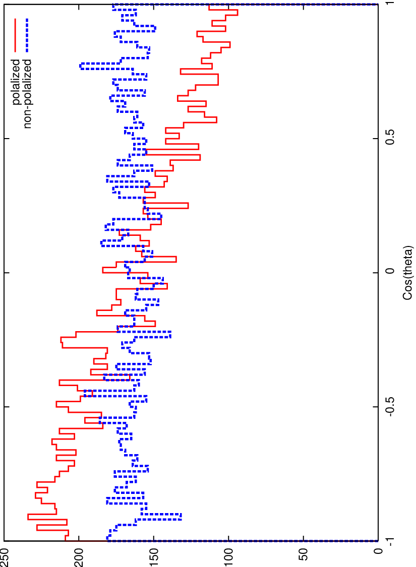

In Fig.9 (left), we show the parton level top decay distribution as the function of for the polarized and non-polarized cases, where is the angle between the -quark momentum and the -quark boost direction at the rest flame of the -quark. We find evident difference between the two cases. In the region around , the emission of quark is suppressed because the amplitude proportional to is suppressed for .
To see this at jet level, we study distributions of jets that are consistent to top decay products. Some parton configuration is difficult to resolve at jet level. We analyse only the hemispheres with GeV GeV. We require that two of the three jets are consistent with those coming from , that is GeV, and the other jet is -tagged. Here, we regard a jet as a -jet if the direction of the momentum is in a cone centered at a bottom parton momentum with GeV. The analysis of the hemisphere which consists of 2 jets is given in Appendix A.3.
In Fig.9 (right) we show the distribution of the angle between the b-jet momentum and the reconstructed top momentum . For the plot, we selected only the events with GeV. Under the cut, Standard Model backgrounds are negligible as seen in Sec.II. We use the measured hemisphere momentum to go back to the rest frame of the jet system. There is a distinguishable difference between polarized and non-polarized distributions. The ratio for the polarized case, while it is for the unpolarized one.
A polarized top quark decays into a polarized . Decay distribution of polarized () can be calculated and the amplitudes are written as follows,
| (21) | |||||
| (22) | |||||
| (23) |
Here, and are the polar and the azimuth angles of the momentum of one of the jets from a decay to the momentum direction. These momenta are defined at the rest frame of the . A longitudinally polarized () tends to decay transversely. On the other hand a transversely polarized () tends to decay along a direction of the momentum.
These differences may appear in the jet asymmetry , which defined as follows,
| (24) |
Jets from a decay tend to have while those from a give larger . This can be seen in Fig.10 (left). In this plot the distributions are shown for the events with . The ratio with is larger for polarized tops. Therefore, for polarized top is distributed more around 0 than for non-polarized top. Fig. 10 (right) shows distributions at jet level for . Unfortunately, It is difficult to see the differences only by the shape of the distribution due to the limited statistics.


V CONCLUSION
In this paper we have studied reconstruction of top quarks arising from productions and its subsequent decay into a top and a stable gauge partner in the LHT. We demonstrate the reconstruction of the top quarks through finding collinear jets whose invariant mass is consistent with using hemisphere analysis. Main SM background processes are jets, jets and jets productions, which can be reduced by imposing the cut on hemisphere momenta and variable.
We also investigate the dependence on jet reconstructing algorithms. The cone algorithm used in the previous study [28] is not optimal for the process. A top from is boosted, while the algorithm is designed so that the highest jets take all activities near the jet, mis-estimating the energy and the direction of the jets. An infrared safe version of the cone algorithms (SISCone) also has some disadvantage for our case, because they tend to merge overlapping jets. We also study distributions with modern clustering algorithms (kt and Cambridge), which in general give better results than the cone algorithms.
We also study effect of underlying events, and find the known tendency that the kt algorithm overestimates jet energies caused by collecting far and soft activities. Whereas the reconstruction efficiency in the Cambridge algorithm is not affected if .
We also discuss top polarization effects. A top quark arising from a top partner decay is naturally polarized. This can be studied through looking into a distribution of the -jet from decay especially the angle to a reconstructed top momentum in the rest frame of the top. We find that difference of the distributions between polarized and non-polarized top is still at detectable level with -tagging for reasonable integrated luminosity (50 fb-1 for GeV and GeV). These analyses are demonstrated using the Cambridge algorithm, which shows good -jet and -parton matching.
In many new physics scenarios, boosted gauge bosons and top quarks are produced at a significant rate. Our study shows that choosing a right jet reconstruction algorithm or studying the dependence on them is important to reveal the physics behind the signal.
Acknowledgement
This work is supported in part by the Grant-in-Aid for Science Research, Ministry of Education, Culture, Sports, Science and Technology, Japan (No.16081207, 18340060 for M.M.N.). This work is also supported by World Premier International Research Center Initiative (WPI Program), MEXT, Japan.
Appendix A Appendix
A.1 Jet smearing
In this paper, we show the distributions without jet energy smearing. In AcerDET, there is an option to smear jet and missing transverse energies. The smearing is introduced for each jet energy in the Snowmass cone algorithm and for a sum of the total transverse momentum (the missing transverse momentum) rather than for each calorimeter cell. We do not try to include smearing effects for the other three jet reconstruction algorithms (kt, Cambridge, SISCone) in this paper, because cells that jets consist of depend on the jet reconstruction algorithms, therefore comparison of smearing effects under the same condition is not easy.
To obtain a rough idea on the signal and background distributions with smearing, we show distributions with/without smearing and jet energy calibration in the Snowmass cone algorithm. The distribution near the end point is not significantly changed. The effect is rather small because we take the smearing based on ATLAS detector performance 50%. which is less than 10 % for jet with 30 GeV.


A.2 Top polarization
In this paper we took mass parameters GeV, GeV, and GeV. The Lagrangian relevant to our study is
| (25) |
Here, and is approximately expressed in terms of
| (26) |
therefore at our model point.
The amplitude of a top partner decay into a top with helicities can be calculated as follows,
| (27) | |||||
| (28) | |||||
| (30) | |||||
where at the rest frame of ,
| (31) | |||||
| (32) | |||||
| (33) | |||||
| (35) |
and,
| (36) | |||||
| (37) |
The is the Wigner’s function,
| (38) |
The square of the amplitudes are therefore expressed for each helicity eigenstate as follows;
| (39) |
Polarization of top quarks from top partner decays is given as follows,
| (40) | |||||
| (42) | |||||
| (44) |
We obtain for our model parameter.
A.3 Jets Configurations in Hemispheres


For hemispheres consistent with a top mass, some parton configurations are difficult to resolve at jet level. We categorize hemispheres with GeV GeV into the following four groups:
-
I. Only one jet in a hemisphere.
-
II. Only two jets in a hemisphere. One of the jets has mass consistent with ( GeV GeV) and the other is -tagged. ( decay products are merged into a jet and -jet is isolated)
-
III. Only two jets in a hemisphere. None of the jets has mass consistent with mass and at least one of jets is -tagged. (One of the partons from decay and a -parton are merged into a jet, and the other from is isolated. )
-
IV. Only three jets in a hemisphere. Invariant mass of two jets is consistent with and the other jet is -tagged.
Here, we regard a jet as a -jet if the direction of the momentum is in a cone centered at a bottom parton momentum with GeV.
In Fig. 12, we plot distribution of jets for each group, where is the angle between a -parton and a -parton momenta at the rest frame of the -parton. The left figure is for non-polarized top quarks and the right figure is for polarized top quarks.
For type IV events, the number of the events where a -parton goes in the forward direction is strongly suppressed for polarized events compared with non-polarized events, while the events for is significantly enhanced. It is consistent with parton level distributions. Note that the events near cannot be accepted as type IV for both polarized and non-polarized cases because of the -parton is too small, while the region is the most sensitive to polarization effects. The other distributions do not show clear dependence on the polarization.
References
- [1] R. Barate et al. [LEP Working Group for Higgs boson searches], Phys. Lett. B 565, 61 (2003) [arXiv:hep-ex/0306033].
- [2] D. N. Spergel et al. [WMAP Collaboration], Astrophys. J. Suppl. 148, 175 (2003) arXiv:astro-ph/0302209.
- [3] D. N. Spergel et al., arXiv:astro-ph/0603449.
- [4] D. G. York et al. [SDSS Collaboration], Astron. J. 120, 1579 (2000) [arXiv:astro-ph/0006396].
- [5] S. Perlmutter et al. [Supernova Cosmology Project Collaboration], Astrophys. J. 517, 565 (1999) [arXiv:astro-ph/9812133].
- [6] A. G. Riess et al. [Supernova Search Team Collaboration], Astron. J. 116, 1009 (1998) [arXiv:astro-ph/9805201].
- [7] R. Barbieri and A. Strumia, arXiv:hep-ph/0007265.
- [8] R. Barbieri and A. Strumia, Phys. Lett. B 462, 144 (1999) [arXiv:hep-ph/9905281].
- [9] C. Csaki, J. Hubisz, G. D. Kribs, P. Meade and J. Terning, Phys. Rev. D 67, 115002 (2003) [arXiv:hep-ph/0211124].
- [10] H. P. Nilles, Phys. Rept. 110, 1 (1984).
- [11] H. E. Haber and G. L. Kane, Phys. Rept. 117, 75 (1985).
- [12] S. P. Martin, arXiv:hep-ph/9709356.
- [13] H. C. Cheng and I. Low, JHEP 0309, 051 (2003) [arXiv:hep-ph/0308199].
- [14] H. C. Cheng and I. Low, JHEP 0408, 061 (2004) [arXiv:hep-ph/0405243].
- [15] I. Low, JHEP 0410, 067 (2004) [arXiv:hep-ph/0409025].
- [16] N. Arkani-Hamed, S. Dimopoulos and G. R. Dvali, Phys. Lett. B 429, 263 (1998) [arXiv:hep-ph/9803315].
- [17] I. Antoniadis, N. Arkani-Hamed, S. Dimopoulos and G. R. Dvali, Phys. Lett. B 436, 257 (1998) [arXiv:hep-ph/9804398].
- [18] I. Antoniadis, Phys. Lett. B 246, 377 (1990).
- [19] T. Appelquist, H. C. Cheng and B. A. Dobrescu, Phys. Rev. D 64, 035002 (2001) [arXiv:hep-ph/0012100].
- [20] J. Hubisz and P. Meade, Phys. Rev. D 71, 035016 (2005) [arXiv:hep-ph/0411264].
- [21] ALTAS Technical Design Report, CERN/LHCC-99-15, ATL-PHYS-98-131 (1998).
- [22] CMS Physics Technical Design Report, CERN/LHCC 2006-001, CMS TDR 8.1 02 February 2006.
- [23] H. Baer, X. Tata and J. Woodside, Phys. Rev. D 45, 142 (1992).
- [24] H. Baer, C. h. Chen, F. Paige and X. Tata, Phys. Rev. D 53, 6241 (1996) [arXiv:hep-ph/9512383].
- [25] A. Belyaev, C. R. Chen, K. Tobe and C. P. Yuan, Phys. Rev. D 74, 115020 (2006) [arXiv:hep-ph/0609179].
- [26] B. Lillie, L. Randall and L. T. Wang, JHEP 0709, 074 (2007) [arXiv:hep-ph/0701166].
- [27] F. Moortgat and L. Pape, CMS Physics TDR Chapter 13.4, p.400-403, CERN/LHCC/2006-021 (26 June 2006).
- [28] S. Matsumoto, M. M. Nojiri and D. Nomura, Phys. Rev. D 75, 055006 (2007) [arXiv:hep-ph/0612249].
- [29] A. Pukhov et al., arXiv:hep-ph/9908288.
- [30] G. Corcella et al., arXiv:hep-ph/0210213.
- [31] P. de Jong, talk at SUSY 2008, Seoul p.19, http://susy08.kias.re.kr/slide/pl/ATLAS_SUSY08_PdJ_bu.ppt
- [32] E. Richter-Was, arXiv:hep-ph/0207355.
- [33] M. Cacciari, arXiv:hep-ph/0607071.
- [34] S. Catani, Y. L. Dokshitzer, M. Olsson, G. Turnock and B. R. Webber, Phys. Lett. B 269, 432 (1991).
- [35] S. Catani, Y. L. Dokshitzer, M. H. Seymour and B. R. Webber, Nucl. Phys. B 406, 187 (1993).
- [36] S. D. Ellis and D. E. Soper, Phys. Rev. D 48, 3160 (1993) [arXiv:hep-ph/9305266].
- [37] M. Cacciari and G. P. Salam, Phys. Lett. B 641, 57 (2006) [arXiv:hep-ph/0512210].
- [38] Y. L. Dokshitzer, G. D. Leder, S. Moretti and B. R. Webber, JHEP 9708, 001 (1997) [arXiv:hep-ph/9707323].
- [39] S. Bentvelsen and I. Meyer, Eur. Phys. J. C 4, 623 (1998) [arXiv:hep-ph/9803322].
- [40] G. P. Salam and G. Soyez, JHEP 0705, 086 (2007) [arXiv:0704.0292 [hep-ph]].
- [41] J. M. Butterworth, J. R. Forshaw and M. H. Seymour, Z. Phys. C 72, 637 (1996) [arXiv:hep-ph/9601371].
- [42] A. Barr, C. Lester and P. Stephens, J. Phys. G 29, 2343 (2003) [arXiv:hep-ph/0304226].
- [43] M. L. Mangano, M. Moretti, F. Piccinini, R. Pittau and A. D. Polosa, JHEP 0307, 001 (2003) [arXiv:hep-ph/0206293].
- [44] W. S. Cho, K. Choi, Y. G. Kim and C. B. Park, arXiv:0711.4526 [].
- [45] A. J. Barr, B. Gripaios and C. G. Lester, JHEP 0802, 014 (2008) [arXiv:0711.4008 [hep-ph]].
- [46] M. Asano, S. Matsumoto, N. Okada and Y. Okada, Phys. Rev. D 75, 063506 (2007) [arXiv:hep-ph/0602157].
- [47] G. Brooijmans, ATLAS NOTE: ATL-COM-PHYS-2008-001
- [48] T. Han, R. Mahbubani, D. G. E. Walker and L. T. E. Wang, arXiv:0803.3820 [hep-ph].
- [49] J. M. Butterworth, A. R. Davison, M. Rubin and G. P. Salam, arXiv:0802.2470 [hep-ph].
- [50] J. Hubisz, P. Meade, A. Noble and M. Perelstein, JHEP 0601, 135 (2006) [arXiv:hep-ph/0506042].
- [51] G. L. Kane, G. A. Ladinsky and C. P. Yuan, Phys. Rev. D 45, 124 (1992).