Analysis of the Karmarkar-Karp Differencing Algorithm
Abstract
The Karmarkar-Karp differencing algorithm is the best known polynomial time heuristic for the number partitioning problem, fundamental in both theoretical computer science and statistical physics. We analyze the performance of the differencing algorithm on random instances by mapping it to a nonlinear rate equation. Our analysis reveals strong finite size effects that explain why the precise asymptotics of the differencing solution is hard to establish by simulations. The asymptotic series emerging from the rate equation satisfies all known bounds on the Karmarkar-Karp algorithm and projects a scaling , where . Our calculations reveal subtle relations between the algorithm and Fibonacci-like sequences, and we establish an explicit identity to that effect.
pacs
02.60.PnNumerical optimization and 89.75.DaSystems obeying scaling laws and 89.75.FbStructures and organization in complex systems1 Introduction
Consider a list of positive numbers. Replacing the two largest numbers by their difference yields a new list of numbers. Iterating this operation times leaves us with a single number. Intuitively we expect this number to be much smaller than all the numbers in the original list. But how small? This is the question that we address in the present paper.
The operation that replaces two numbers in a list by their difference is called differencing, and the procedure that iteratively selects the two largest numbers for differencing is known as largest differencing method or LDM. This method was introduced in 1982 by Karmarkar and Karp [1] as an algorithm for solving the number partitioning problem (Npp): Given a list of positive numbers, find a partition, i.e. a subset such that the discrepancy
| (1) |
is minimized. Obviously, LDM amounts to deciding iteratively that the two largest numbers will be put on different sides of the partition, but to defer the decision on what side to put each number. The final number then represents the discrepancy.
Despite its simple definition, the Npp is of considerable importance both in theoretical computer science and statistical physics. The Npp is NP-hard, which means (a) that no algorithm is known that is essentially faster than exhaustively searching through all partitions, and (b) that the Npp is computationally equivalent to many famous problems like the Traveling Salesman Problem or the Satisfiability Problem [2]. In fact, the Npp is one of Garey and Johnson’s six basic NP-hard problems that lie at the heart of the theory of NP-completeness [3], and it is the only one of these problems that actually deals with numbers. Hence it is often chosen as a base for NP-hardness proofs of other problems involving numbers, like bin packing, multiprocessor scheduling [4], quadratic programming or knapsack problems. The Npp was also the base of one of the first public key crypto systems [5].
In statistical physics, the significance of the Npp results from the fact that it was the first system for which the local REM scenario was established [6, 7]. The notion local REM scenario refers to systems which locally (on the energy scale) behaves like Derrida’s random energy model [8, 9]. It is conjectured to be a universal feature of random, discrete systems [10]. Recently, this conjecture has been proven for several spin glass models [11, 12] and for directed polymers in random media [13].
Considering the NP-hardness of the problem it is no surprise that LDM (which runs in polynomial time) will generally not find the optimal solution but an approximation. Our initial question asks for the quality of the LDM solution to Npp, and to address this question we will focus on random instances of the Npp where the numbers are independent, identically distributed (i.i.d.) random numbers, uniformly distributed in the unit interval. Let denote the output of LDM on such a list. Yakir [14] proved that the expectation is asymptotically bounded by
| (2) |
where and are (unknown) constants such that
| (3) |
In this contribution we will argue that .
The paper is organized as follows. We start with a comprehensive description of the differencing algorithm, a simple (but wrong) argument that yields the scaling (2) and a presentation of simulation data that seems to violate the asymptotic bound (3). In section 3 we reformulate LDM in terms of a stochastic recursion on parameters of exponential variates. This recursion will then be simplified to a deterministic, nonlinear rate equation in section 4. A numerical investigation of this rate equation reveals a structure in the dynamics of LDM that can be used as an Ansatz to simplify both the exact recursions and the rate equation. This will lead to a simple, Fibonacci like recursion (section 5) and to an analytic solution of the rate equation (section 6). In both cases we can derive the asymptotics including the corrections to scaling, and we claim that a similar asymptotic expansion holds for the original LDM. The latter claim is corroborated by fitting the asymptotic expansion to the available numerical data on LDM.
2 Differencing Algorithm
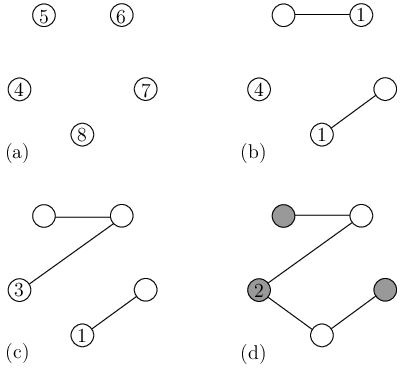
The differencing scheme as described in the introduction gives the value of the discrepancy, but not the actual partition. For that we need some additional bookkeeping, which is most easily implemented in terms of graphs (Fig. 1). The algorithm maintains a list of rooted trees where each root is labeled with a number. The algorithm starts with trees of size one and the roots labeled with the numbers . Then the following steps are iterated until a single rooted tree of size remains:
- 1.
Among all roots, find those with the largest () and second largest () label.
- 2.
Join nodes and with an edge, declare node as the root of the new tree and relabel it with .
After iterations all nodes are spanned by a tree whose root is labeled by the final discrepancy. This tree can easily be two-colored, and the colors represent the desired partition.
Fig. 1 illustrates this procedure on the instance . The final two coloring corresponds to the partition versus with discrepancy . Note that the optimum partition versus achieves discrepancy .
Technically, LDM boils down to deleting items from and inserting items into a sorted list of size . This can be done in time using an advanced data structure like a heap [15]. Hence LDM is very efficient, but how good is it? As we have already seen in the example, LDM can miss the optimal partition. And for random instances, the corridor (2) is far above the true optimum, which is known to scale like [7]. Yet LDM yields the best results that can be achieved in polynomial time. Many alternative algorithms have been investigated in the past [16, 17], but they all produce results worse than (2). The few algorithms that can actually compete with the Karmarkar-Karp procedure use the same elementary differencing operation [18, 19]. It seems as if the differencing scheme marks an inherent barrier for polynomial time algorithms.
The following argument explains the scaling (2). The typical distance between adjacent pairs of the numbers in the interval is . Hence after differencing operations we are left with numbers in the interval . The typical distance between pairs is now . After another round of differencing operations we get numbers in the range . In general, after differencing operations we are left with numbers in the range . Reducing the original list to a single number requires differencing operations, and applying the above argument all the way down suggests that
| (4) |
with
| (5) |
As we will see, this is the right scaling, yet the argument cannot be correct. This follows from the fact that it predicts the same scaling for the paired differencing method (PDM). Here in each round all pairs of adjacent numbers are replaced by their difference in parallel. This method, however, yields an average discrepancy of order [20]. Yet, our analysis below suggests that (4) and (5) indeed describe the asymptotic behavior correctly, although a far more subtle treatment is required.

An obvious approach to find the quality of LDM are simulations. We ran LDM on random instances of varying size , and Figure 2 shows the results for . Apparently scales like , in agreement with (2) and (4). A linear fit seems to yield
for the constant in (4), which clearly violates the bound . Apparently even is too small to see the true asymptotic behavior. This may be the reason why Monte Carlo studies of LDM never have been published.

A plot of the probability density function (pdf) of reveals a data collapse varying values of (Fig. 3). Apparently the complete statistics of is asymptotically dominated by a single scale .
Some technical notes about simulating LDM are appropriate. Differencing means subtracting numbers over and over again. The numerical precision must be adjusted carefully to support this and to be able to represent the final discrepancy of order . We used the freely available GMP library [21] for the required multiple precision arithmetic and ran all simulations on -bit integers where the number of bits ranges from (for ) to for . The integer discrepancies were then rescaled by . The pseudo random number generator was taken from the TRNG library [22].
3 Exact Recursions
A common problem in the average-case analysis of algorithms like LDM is that numbers become conditioned and cease to be independent as the algorithm proceeds. Lueker [20] proposed to use exponential instead of uniform variates to cope with this problem. Let be i.i.d. random exponentials with mean and consider the partial sums . Then the joint distribution of the ratios , , is the same as that of the order statistics of i.i.d. uniform variates from [23]. As a consequence, LDM will produce the same distribution of data no matter whether it is run on uniform variates or on . Let denote the result of LDM on the partial sums . Since the output of LDM is linear in its input, we have
| (6) |
where is the sum of i.i.d. exponential variates and the notation indicates that the random variable and have the same distribution. The probability density of is the gamma density
| (7) |
Taking expectations of both sides of (6) we get
| (8) |
This allows us to derive the asymptotics of from the asymptotics of .
Exponential variates are well suited for the analysis of LDM because the sum and difference of two exponential variates are again exponential variates. Once started on exponential variates, LDM keeps working on exponentials all the time. This allows us to express the operation of LDM in terms of a recursive equation for the parameters of exponential densities [14]. We start with the following Lemma:
Lemma 1
Let and be independent exponential random variables with parameter and , resp.. The probability of the event is given by
| (9) |
Furthermore, conditioned on the event , the variables and are independent exponentials with parameters (for ) and for .
The proof of Lemma 1 consists of trivial integrations of the exponential densities and is omitted here.
Next we consider generalized partial sums of exponentials, described by -tuples
This -tuple is shorthand for the sequence of partial sums
with .
Now let us look at the result of one iteration of LDM on . The two largest numbers are removed and replaced by their difference which is an variate. Lemma 1 tells us, that the probability that this number is the smallest in the list is
and conditioned on that event, the smallest number is an variate and the increment to the 2nd smallest number is an independent variate. Conditioned on we get another -tuple as the input for the next iteration:
The probability that is
and in this case is an variate, whereas the difference is an variate. Now the probability that the new number is second in the new list reads
and conditioned on that event the input for the new iteration is
This argument can be iterated to calculate the probability of becoming the -th number in the new list. Denoting the partial sums by we get
| (10) |
for and conditioned on that event the new list is
| (11) |
The final case is that becomes the largest number in the new list. This happens with probability
| (12) |
and leads to the list
| (13) |
In all cases we stay within the set of instances given by partial sums of independent exponentials, and we can apply Eqs. (10) to (13) recursively until we have reduced the original problem to a -instance which tells us that the final difference is an variate.

| 4 | 5 | 6 | 7 | 8 | |
|---|---|---|---|---|---|
| 1 | |||||
| 2 | |||||
| 3 | |||||
| 4 | |||||
| 5 | |||||
| 6 | |||||
| 7 | |||||
| 8 | |||||
| 9 | |||||
| 10 | |||||
| 11 | |||||
| 12 | |||||
| 13 |
Fig. 4 shows the result of this analysis on the input , our original problem with . We have to explore the tree that branches according to the position that is taken by the new number inserted in the shortened list. The numbers written on the edges of the tree are the probabilities for the corresponding transition. Note that we have combined the two branches emerging from the root that both lead to a -configuration into a single one by adding their probabilities. In the end we get
for the probability density function (pdf) of . In general, the pdf of is a sum of exponentials,
| (14) |
where is the probability of LDM returning an -variate. For small values of , this probabilities can be calculated by expanding the recursions explicitly (Table 1), but for larger values of this approach is prohibited by the exponential growths of the number of branches that have to be explored.

Alternatively we can explore the tree of -tuples by walking it randomly. Given a tuple , we generate a random integer with probability
| (15) |
and using this random we generate a new tuple of size according to Eqs. (11) or (13). This process is iterated until the tuple size is two, and the final value of is the parameter for the statistics of . The probability density of is shown in Fig. 5). Again the data collapse corroborates the claim that the statistics of is dominated by a single scale.
4 Rate Equation
We can turn the exact recursions from Sec. 3 into a set of rate equations for the time-evolution of the average -tuple. Let denote the value of after iterations, such that
| (16) |
As explained in Sec. 3, at “time” a number , is chosen with probability
| (17) |
Depending on the choice of , Eqs. (11) and (13) suggest that only takes on one of two possible values. For , these are
| (18) |
whereas for , the two values are
| (19) |
We introduce the shorthand
| (20) |
for the probability of at iteration . On average, the evolution of is given by the rate equation
| (21) |
for all , and at the upper boundary
| (22) |
These equations are defined on the triangular domain , . The initial conditions are
| (23) |
As described in Sec. 3, the process terminates at with characterizing the exponential variate for the final difference in LDM. Yet, Eq. (22) for implies , reflecting the final, trivial differencing step, and it will prove conceptually advantageous to focus on the asymptotic properties of instead.
Since the rate equation is an approximation to the exact recursion, we need to check how accurate it is. We have solved the rate equations (21-23) numerically up to . Fig. 8 shows
from the rate equation versus . If were calculated as an average from the exact recursion, it should be equal to
from the direct simulation of LDM. Fig. 8 shows this quantity, too. Apparently the error introduced by approximating the exact recursion by the rate equation vanishes for , and our conjecture is that the rate equation and the exact recursion are asymptotically equivalent. Judging from our numerical studies below, see Tab. 2, both asymptotic series have a relative difference of size .
The time to solve the rate equation numerically scales like , so it is actually more efficient to simulate LDM directly, not least because the sampling for the latter can be done efficiently on a parallel machine. For analytic approaches, however, the rate equation is more convenient.

The initial probabilities decay exponentially,
| (24) |
which implies that only the first values increase. Everywhere else, is essentially zero, and those entries will not increase until the first term of (21) has copied the values from the low index boundary. Hence we expect a “wavefront” of increased -values to travel with a velocity one index per time step toward the upper boundary, which in turn travels with the same velocity towards the lower boundary. As can be seen from Fig. 6, this traveling wavefronts of increasing heights are a hallmark of the rate equation for all times . We will use this intuitive picture for an Ansatz to analyze both the exact recursion and the rate equation in the next two sections.
5 Fibonacci Model
Both the exact recursion and the rate equations yield
| (25) |
for the lower boundary that we are ultimately interested in. This recursion connects the lower and the upper boundaries at and at . Unfortunately, depends in a complicated way on entries of the -tuple at different times and different places. However, Fig. 6 suggests a similarity Ansatz
| (26) |
which makes the upper boundary readily available:
| (27) | |||||
Note that we have extended the initial conditions to hold for all negative times, too.

It turns out that one can express the final value of this recursion in terms of the corresponding values in smaller systems, which leads to a simple recursion in . To derive this recursion it is convenient to visualize (27) in terms of paths in a right-angled triangle (Fig. 7). The hypotenuse of represents and ranges from to , the height is . Let us discuss the basic mechanism for the example . The final recursion reads
and the two terms on the right hand side correspond to two paths: one that connects 6 with 7 along the hypotenuse, the other connects 5 with 7 along the path that is “reflected” at the right leg of . In our case a reflected path moves diagonally upward until it touches the right leg above point . From there it moves downward to point . This peculiar “law of refraction” implies that only every second point of the left half of the hypotenuse is connected to the right half by a reflected path.
We can apply the recursion again and write
Here we have connected with along the hypotenuse and with along a reflected path, and similarly for . We iterate this path finding process until all paths end on the left half of the hypotenuse (negative ). Here the paths collect the initial values , hence equals the number of different paths that connect the points to the point on the hypotenuse. Instead of considering each paths that starts on the left half of the hypotenuse separately we let all paths start in the leftmost point . The rule for path finding then is: if you are on an even index, move one unit to the right. If you are on an odd index, there are two branches: one to the right, the other 45 degrees upward and reflected down to the hypotenuse. Obviously, equals the number of different paths that connects the leftmost point of to the rightmost point according to this rules. Let denote the number of paths that connect the point with in . Then we have
Now, starting at , we have two choices: move upward for a reflection that will take us to point or move along the hypotenuse to point :
As we can see in Fig. 7 (top), the number of paths from to is exactly the same as the total number of paths in . Hence
Similarly, the number of paths from to equals the total number of paths in a slightly smaller triangle, as can be seen in Fig. 7 (bottom). Hence we have
and all three equations yield
The derivation of a corresponding equation for odd values of is straightforward. If we define
| (28) |
the recursion for translates into the Fibonacci like recursion
| (29) | ||||
where refers to the integer part of . The resulting sequence is known as A033485 in [24]. The generating function satisfies the functional equation
| (30) |
and is given by
| (31) |
can be evaluated numerically for values of that are larger than the values feasible for simulations of LDM or for solving the rate equation. The bottleneck for calculating is memory, not CPU time, since values must be stored to get . With 3 GByte of memory, we managed to calculate for . We will derive the asymptotics of in the next section.
Fig 8 shows within the same scaling as the simulations of LDM and the numerical solution of the rate equation. Apparently the similarity Ansatz does not capture the full complexity of the LDM algorithm or the rate equation. Yet it yields a very similar qualitative behavior. And in the next section we will show that
| (32) |

6 Continuum Limit
To analyze the rate equations (21-23), it is convenient to consider the continuum limit for . Asymptotically, a continuum solution may differ from the discrete problem in corrections of order . As we will see, such corrections are inaccessible, as the asymptotic expansion is a series in terms of .
We rewrite Eq. (21) in terms of discrete differences,
| (33) |
Setting
| (34) | |||||
we obtain for large
| (35) |
where we have set
| (36) |
with
| (37) |
The left-hand side of Eq. (35), as well as the numerical solution of the full rate equations (21-23) displayed in Fig. 6, again suggest a similarity Ansatz
| (38) |
This Ansatz yields immediately for Eq. (35):
| (39) |
For almost all , the right-hand side vanishes by virtue of , as indicated by Eq. (36) for and . Correspondingly, at the upper boundary, which justifies the similarity solution for the continuum limit of Eq. (22). Yet, for all , hence we are left with
| (40) |
which can be interpreted as the continuous version of (27). From the initial conditions of the discrete problem in (23) it is clear that . For the similarity solution, this implies that
| (41) |
Integrating (40), we formally obtain
| (42) |
Thus, we can evaluate the integral for to get
| (43) |
We can continue this process for , i. e., , exactly the domain of validity of (43), to obtain
| (44) | |||||
The emergent pattern is best represented by defining
| (45) |
for , where Eqs. (41-44) represent , and . In general, we find that
| (46) |
which is solved by
| (47) |
For any , we are interested in , hence
| (48) |
which concludes our solution of (40). The sum for still depends on , hence we define
| (49) |
Now can be evaluated numerically for very large values of . Fig. 8 shows the result for . Don’t try this at home unless you have a computer algebra system. Interestingly, asymptotically approaches a value that is extremely close to . In fact, an asymptotic analysis (see Appendix) reveals
| (50) | ||||
which is the dashed line in Fig. 8. The dotted lines are numerical least square fits of the terms of this scaling, i.e., fits of the form
| (51) | ||||
with values for as shown shown in Table 2.
7 Conclusion
The numerical data supports the claim that the complete statistics of LDM is dominated by a single scale , not just the expectation as described in (2). The available data is not sufficient to pin down the precise asymptotic scaling, however. In fact a naive extrapolation of the available data even contradicts the known asymptotic bound (3). With its complexity, LDM is a very efficient algorithm, but probing the asymptotics requires to be large. This discrepancy of scales eliminates simulations as a means to study the asymptotics of LDM and calls for alternative approaches.
We have taken a step in the direction of a rigorous asymptotic analysis by mapping the differencing algorithm onto a rate equation. The structure seen in the evolution of this rate equation (Fig. 6) suggests a similarity Ansatz (26). With the help of this Ansatz we could reduce the exact recursion in -space to the Fibonacci model (29). The asymptotics of this model can be calculated, and it agrees with (2) and (3). The same Ansatz plugged into the rate equation even allows us to calculate the first terms of an asymptotic expansion (50). Although our Ansatz does not yield a proof, the extracted asymptotic behavior satisfies all previous constraints and provides a consistent interpretation of the numerical results. Hence, our rate equations pave the way for further systematic investigations.
Acknowledgements.
We appreciate stimulating discussions George E. Hentschel and Cris Moore. S.M. enjoyed the hospitality of the Cherry L. Emerson Center for Scientific Computation at Emory University, where part of this work was done. Most simulations were run on the Linux-Cluster Tina at Magdeburg University. S.M. was sponsored by the European Community’s FP6 Information Society Technologies programme, contract IST-001935, EVERGROW.Appendix A Asymptotic Analysis
To evaluate the series (49) we apply Laplace’s saddle-point method for sums as described on p. 304 of Ref. [26]. For
the saddle point is determined by , i. e., , or
| (52) |
Hence, we obtain a moving (-dependent) saddle point at
| (53) |
including terms to the order needed to determine up to the correct prefactor. We keep the -corrections, since contains terms like . In particular, it is
| (54) |
As the saddle point is large for large , we can replace by its Stirling-series [26]. Then, we expand around the saddle point by substituting , keeping only terms to 2nd order in and those that are non-vanishing for . We find
with log-polynomial corrections
| (55) | ||||
We finally obtain for the asymptotic expansion of (50):
| (56) | |||||
References
- [1] Narendra Karmarkar and Richard M. Karp. The differencing method of set partitioning. Technical Report UCB/CSD 81/113, Computer Science Division, University of California, Berkeley, 1982.
- [2] Stephan Mertens and Cristopher Moore. The Nature of Computation. Oxford University Press, Oxford, 2008.
- [3] Michael R. Garey and David S. Johnson. Computers and Intractability. A Guide to the Theory of NP-Completeness. W.H. Freeman, New York, 1997.
- [4] Heiko Bauke, Stephan Mertens, and Andreas Engel. Phase transition in multiprocessor scheduling. Phys. Rev. Lett, 90(15):158701, 2003.
- [5] R. C. Merkle and M. E. Hellman. Hiding informations and signatures in trapdoor knapsacks. IEEE Transactions on Information Theory, 24:525–530, 1978.
- [6] Stephan Mertens. Random costs in combinatorial optimization. Phys. Rev. Lett., 84(6):1347–1350, February 2000.
- [7] Christian Borgs, Jennifer Chayes, and Boris Pittel. Phase transition and finite-size scaling for the integer partitioning problem. Rand. Struct. Alg., 19(3–4):247–288, 2001.
- [8] Bernard Derrida. Random-energy model: Limit of a family of disordered models. Phys. Rev. Lett., 45:79–82, 1980.
- [9] Bernard Derrida. Random-energy model: An exactly solvable model of disordered systems. Phys. Rev. B, 24(5):2613–2626, 1981.
- [10] Heiko Bauke and Stephan Mertens. Universality in the level statistics of disordered systems. Phys. Rev. E, 70:025102(R), 2004.
- [11] Anton Bovier and Irina Kurkova. Local energy statistics in disordered systems: a proof of the local REM conjecture. Commun. Math. Phys., 263:513–533, 2006.
- [12] Anton Bovier and Irina Kurkova. Local energy statistics in spin glasse. J. Stat. Phys., 126:933–949, 2007.
- [13] Irina Kurkova. Local energy statistics in directed polymers. Electronic Journal of Probability, 13:5–25, 2008.
- [14] Benjamin Yakir. The differencing algorithm LDM for partitioning: a proof of a conjecture of Karmarkar and Karp. Math. Oper. Res., 21(1):85–99, 1996.
- [15] Jon Kleinberg and Éva Tardos. Algorithm Design. Addison Wesley, Boston, 2006.
- [16] David S. Johnson, Cecicilia R. Aragon, Lyle A. McGeoch, and Catherine Schevron. Optimization by simulated annealing: an experimental evaluation; part II, graph coloring and number partitioning. Operations Research, 39(2):378–406, May-June 1991.
- [17] W. Ruml, J.T. Ngo, J. Marks, and S.M. Shieber. Easily searched encodings for number partitioning. Journal of Optimization Theory and Applications, 89(2):251–291, May 1996.
- [18] Richard E. Korf. A complete anytime algorithm for number partitioning. Artificial Intelligence, 106:181–203, 1998.
- [19] Robert H. Storer, Seth W. Flanders, and S. David Wu. Problem space local search for number partitioning. Annals of Operations Research, 63(4):465–487, 1996.
- [20] George S. Lueker. A note on the average-case behavior of a simple differencing method for partitioning. Oper. Res. Lett., 6(6):285–287, 1987.
- [21] The GNU Multiple Precision Arithmetic Library. http://gmplib.org.
- [22] TRNG - portable random number generators for parallel computing. http://trng.berlios.de/.
- [23] William Feller. An Introduction to Probability and Its Applications, volume 2. John Wiley & Sons, 2 edition, 1972.
- [24] N.J.A. Sloane. The on-line encyclopedia of integer sequences. http://www.research.att.com/~njas/sequences.
- [25] Cristopher Moore and Porus Lakdawala. Queues, stacks, and transcendentality at the transition to chaos. Physica D, 135:24–40, 2000.
- [26] Carl M. Bender and Steven A. Orszag. Advanced Mathematical Methods for Scientists and Engineers. McGraw-Hill, New York, 1978.