Generating functions for coluored 3D Young diagrams and the Donaldson-Thomas invariants of orbifolds
Abstract.
We derive two multivariate generating functions for three-dimensional Young diagrams (also called plane partitions). The variables correspond to a colouring of the boxes according to a finite abelian subgroup of . These generating functions turn out to be orbifold Donaldson–Thomas partition functions for the orbifold . We need only the vertex operator methods of Okounkov–Reshetikhin–Vafa for the easy case ; to handle the considerably more difficult case , we will also use a refinement of the author’s recent –enumeration of pyramid partitions.
In the appendix, we relate the diagram generating functions to the Donaldson-Thomas partition functions of the orbifold . We find a relationship between the Donaldson-Thomas partition functions of the orbifold and its -Hilbert scheme resolution. We formulate a crepant resolution conjecture for the Donaldson-Thomas theory of local orbifolds satisfying the Hard Lefschetz condition.
1. Introduction
A 3D Young diagram, or 3D diagram for short, is a stable pile of cubical boxes which sit in the corner of a large cubical room. More formally, a 3D Young diagram is a finite subset of such that if any of
are in , then . The ordered triples are the “boxes”; the closure condition means that the boxes of a 3D partition are stacked stably in the positive octant, with gravity pulling them in the direction .
3D Young diagrams are well–studied; they are also called plane partitions or 3D partitions elsewhere in the literature. The first result on 3D Young diagrams is due to Dr. Percy MacMahon [19]. MacMahon was the first to “–count” (i.e. to give a generating function for) 3D Young diagrams by volume:
| (1) |
where denotes the number of boxes in . Generating functions of this form will appear frequently, so we adopt the following notation:
Definition 1.1.
Let
We call and the MacMahon and MacMahon tilde functions, respectively. Strictly speaking, lies in the ring of formal power series . However, in all of our applications, we will specialize and in such a way that no negative powers of any variables appear in the formulae (see Theorems 1.4 and 1.5).
Since MacMahon, there have been many proofs of (1), spanning many fields: combinatorics, statistical mechanics, representation theory, and others. Recently, there has been a thorough study of the various symmetry classes of 3D Young diagrams [5], and of many macroscopic properties of large random 3D Young diagrams [25]. There is also active research in algebraic geometry which relies upon enumerations of various types of 3D partitions [20].
We will derive two refinements of MacMahon’s generating function. Fix a set of colours , and replace the variable with a set of variables,
We will need to assign a colour to each point of the first orthant. In particular, we will usually have , a finite Abelian group. In this case, addition in must respect the group law of .
Definition 1.2.
A colouring is a map
If is a finite Abelian group, then a –colouring is a colouring which is also a homomorphism of additive monoids.
Note that a –colouring is uniquely determined by , and , and that is the identity element of .
There is a simple way of defining a –colouring when is a three–dimensional matrix group . Decompose as a direct sum of one–dimensional representations . The set of irreducible representations of any Abelian forms a group under tensor product, so let be an isomorphism and define
Both of the colourings used in this paper are of this form.
We next define the multivariate generating function which “–counts” diagrams (that is, counts each diagram with the –weight of its boxes):
Definition 1.3.
For , let be the number of –coloured boxes in ,
Define the -coloured partition function
The question of determining , though completely combinatorial, has its genesis in a field of enumerative algebraic geometry called Donaldson-Thomas theory. When is a finite Abelian subgroup of (which forces or ), there is a colouring induced by the natural three dimensional representation for which the generating function is, up to signs of the variables, the orbifold Donaldson–Thomas partition function for the quotient stack (see Appendix A). Although it is not yet clear why, these seem to be precisely the groups for which has a product formula.
Theorem 1.4.
Let and let the colouring be given by
Let and for , let . Then
The proof of Theorem 1.4 is straightforward; it is essentially a simple modification of the methods used in [27] (or, indeed, a special case of the extremely general methods of [25]). We include it for completeness and as an introduction to the vertex operator calculus used to prove Theorem 1.5. There are several other ways to prove Theorem 1.4, some of which have (at least implicitly) appeared in the literature. For example, [1, 14] both compute a generating function with variables which can be easily specialized to . The result [1] is particularly notable, as it is a direct computer algebra implementation of MacMahon’s techniques of combinatory analysis. The following theorem, however, is new:
Theorem 1.5.
Let and let the colouring be given by
Let . Then
See Figure 1 for pictures of a partition coloured in the manner described by these theorems.


As an application of these theorems, we will compute the Donaldson-Thomas invariants of the orbifolds and . The orbifold Donaldson-Thomas partition function of has variables labeled by representations of (see Appendix) and hence has the same variables as the -coloured diagram partition function. In the Appendix, we prove that the diagram partition function and the Donaldson-Thomas partition function are related by simple sign changes on the variables:
Theorem 1.6.
There is a striking similarity between the Donaldson-Thomas partition functions of the orbifold and the crepant resolution given by the –Hilbert scheme. The following is proved in the Appendix:
Theorem 1.7.
Let be the crepant resolution of given by the -Hilbert scheme. has a natural basis of curve classes indexed by non-trivial elements of . The Donaldson-Thomas partition functions of and are given by
where and are the variables corresponding to curve classes and is the variable corresponding to Euler number.
We see from these theorems that the reduced partition function of the orbifold is obtained from the reduced partition function of the resolution by identifying the variables appropriately and then simply writing a tilde over every factor of in the formula! A similar phenomenon was observed by Szendrői for the partition function of the (non–commutative) conifold singularity and its crepant resolution [31].
It would be very desirable to have even a conjectural understanding of the relationship between the Donaldson–Thomas theory of an arbitrary Calabi–Yau orbifold and its crepant resolution(s). We formulate a conjecture for the case of a local orbifold satisfying the hard Lefschetz condition (see Conjecture A.6.
Theorem 1.5 is not straightforward to prove. Essentially none of the standard proofs of MacMahon’s colourless result can be modified to work in this situation. The generating function was first conjectured by Jim Bryan based on some related phenomena from Donaldson–Thomas theory; concurrently, Kenyon made an (unpublished) equivalent conjecture for –weighted dimer models on the hexagon lattice, based on computational evidence.
Having this conjectured formula was crucial for finding the proof of Theorem 1.5, which involves a somewhat bizarre detour: one must first –count pyramid partitions (see Figure 4). One then performs a computation with vertex operators to make emerge. We discovered this idea serendipitously while trying to generalize our earlier work on pyramid partitions [32].
2. Review: the infinite wedge space
Our general strategy will be to think of a 3D diagram as a set of diagonal slices, , where is the set of all bricks which lie in the plane . We will then analyze how one passes from one slice to the next. Since we will be summing over all 3D Young diagrams, it is very helpful to consider (possibly infinite) formal sums of the form
where is a power series in the elements of . A nice way of describing the set of all such sums is the charge–zero subspace of the infinite wedge space,
where is a vector space with a basis labeled by the elements of . This setting allows one to define, quite naturally, several useful operators on partitions.
The use of , and its associated operators, was in part popularized by [24, Appendix A], and we shall adhere to the notation established there. In this section, we have collected the minimum number of formulae necessary for our purposes. We will use Dirac’s “bra–ket” notation
to denote the inner product under which the partitions are orthonormal. We will need need the bosonic creation and annihilation operators , defined in [24, Appendix A] in the section on Bosons and Vertex Operators. The operators satisfy the Heisenberg commutation relations,
| (2) |
Concretely, acts on a 2D Young diagram by adding a single border strip of length onto in all possible ways, with sign , where is the height of the border strip (see Figure 2). The operator is adjoint to , and acts by deleting border strips.
Let be indeterminates; and define the homogeneous, elementary, and power sum symmetric functions as usual:
For a comprehensive reference on symmetric functions, see [30]. We next define the vertex operators :
Definition 2.1.
The matrix coefficients (with respect to the orthonormal basis formed by the 2D Young diagrams) of the operators turn out [24, A.15] to be the skew Schur functions,
We will need the following well-known theorem from representation theory (see, for example, [13, Chapter 8]) to work with and other exponentiated operators.
Theorem 2.2.
(Campbell-Baker-Hausdorff) If and are operators, then
where the higher–order terms are multiples of nested commutators of and .
It is certainly possible to give more terms in the expansion, but we shall only need the following two corollaries.
Corollary 2.3.
If and are commuting operators, then
Corollary 2.4.
If and are operators such that is a central element, then we have
3. The operators , , and
Our next goal is to define precisely what it means for two diagonal slices to sit next to one another in a 3D Young diagram, and to define operators for working with such slices.
Definition 3.1.
Let be two 2D Young diagrams. We say that interlaces with , and write , if and the skew diagram contains no vertical domino.
For example, , because the skew diagram has no two boxes in the same column. The following lemma is easy to check:
Lemma 3.2.
The following are equivalent:
- (1)
.
- (2)
The row lengths satisfy .
- (3)
, for each pair of columns .
- (4)
and are two adjacent diagonal slices of some 3D Young diagram.
Note that we have used the convenient, but slightly nonstandard, notation to denote the columns of .
Part (3) will become relevant in Section 5, when we will see that adjacent diagonal slices of a pyramid partition also interlace.
We are mainly interested in two specializations of which create interlacing partitions, and which depend only upon a single indeterminate . The first will be denoted , and is obtained by performing the specialization , for . Its formula is
| (3) |
Recall [30, Chapter 7] that if are partitions, then we may define the skew Schur function by , where runs over the set of semistandard tableaux of shape . Following [27], we see that
One can then show [26] that
| (4) |
For the second specialization, recall that there is an involution on the algebra of symmetric functions [30, Chapter 7.6], given by any one of the following equivalent definitions:
Here, is the transpose partition of . To obtain the second specialization, called , we first perform the involution and then specialize as before. We obtain the formula
| (5) |
with the property that
Lemma 3.3.
If and are commuting variables, then we have the following multiplicative commutators in :
Proof.
We next define diagonal operators for assigning weights to 2D partitions.
Definition 3.4.
For , define the weight operator by
The operator can be commuted past any of the operators, at the expense of changing the argument of :
4. Counting with colouring
As a motivating example, let us use (3) to write down a vertex operator expression which computes MacMahon’s generating function (1), using the variable . This formula appears in [27] with marginally different notation.
Consider a 3D Young diagram and its diagonal slices:
where denotes the empty partition. Each such contributes
to the generating function, so we have
This works because the operators and pass from one slice to the next larger (respectively smaller) slice in all possible ways, and the operators assign the proper weight to each slice. One then commutes all the operators to the left and all the operators to the right (following the method outlined in [27]) to compute the generating function.
Let us now write down a vertex operator expression which computes . Here, , , and . The computation is straightforward (following precisely the method of [27]) but awkward, so it is helpful to organize the work by collecting together vertex operators at a time. Note that the diagonal slices of are all monochrome (see Figure 3), so we define


Then, the following vertex operator product counts –coloured 3D diagrams:
| (6) |
Let , and let . We use the commutation relations of the previous section to compute
Next, set
From this expression, it is clear that
where is the following product of the commutators obtained by moving a past a :
We now follow the derivation of MacMahon’s formula in [27]. Starting with (6), we convert all of the into and move the resulting weight functions to the outside of the product (where they act trivially). This gives
We then commute all operators to the right and all to the left:
The vertex operator product in the final line is now equal to 1, because and . Finally, we rewrite the remaining product with MacMahon functions:
and Theorem 1.4 is proven.
5. Pyramid partitions


The methods of the Section 4 may also be used to -count a similar type of three-dimensional combinatorial object, called pyramid partitions. Essentially, we want to replace with the upside–down pyramid shaped stack of bricks shown in Figure 4. Note that the bricks have ridges and grooves set into them; this helps to remind us how the bricks are meant to stack.
Szendrői [31] introduced us to the ideas in this section, albeit in a different context. He proves that counting pyramid partitions with a slightly simpler colour scheme (namely specializing ) yields a certain noncommutative Donaldson–Thomas partition function. We shall borrow some of Szendrői’s terminology, but not much of the machinery that he developed.
We will start by giving a rather algebraic definition for the bricks in a pyramid partition. Consider the quiver (or directed graph) shown in Figure 5(a). The vertices of are the elements of . The edges are labelled .
Definition 5.1.
A word in is the concatenation of the edge labels of some directed path in . We may optionally associate a base to a word; the base is the starting vertex of the path.
Note that a word based at may also be based at , but not at or . Any path in is uniquely determined by its base and its word.
Definition 5.2.
Form the path algebra spanned by all words in , and define the noncommutative quotient ring , where
If is a word in , we write for its residue class in .
Definition 5.3.
A brick is an element of , where is a word based at the vertex 0. Let be the set of all bricks.

To understand how to draw Figure 4, we interpret the edge labels of as vectors in .
Definition 5.4.
Let
The position of a brick is the sum of the vectors corresponding to the edge labels in . The brick corresponding to the empty walk, , is located at the origin.
We next define a “colouring” on .
Definition 5.5.
Define
by setting to be the final vertex of any path whose word is . We call the colour of .
For an example of all of these concepts, define the brick by the word . The brick is based at the vertex , ending at the vertex . The position of is ; is the -coloured brick in the top layer of Figure 5b.
Note that the colour is completely determined by the and coordinates of ; Figure 6 shows the colouring as viewed from along the axis.
Definition 5.6.
A pyramid partition is a subset of such that if then every prefix of also represents a brick in .
Note that pyramid partitions may also be defined algebraically, although it is unnecessary to do so for this paper. A pyramid partition corresponds to a framed cyclic –module based at 0, much in the same way that a 3D Young diagram corresponds to a monomial ideal in . We refer the reader to [31] for further details of this approach.
Our next goal is to show that the diagonal slices of a pyramid partition interlace with one another. This will allow us to reuse the strategy of Section 4 to obtain a nice generating function for pyramid partitions.
Definition 5.7.
Let be a pyramid partition. Define the th diagonal slice of , written , to be the set of all bricks in whose position satisfies .
Lemma 5.8.
Let . Then
where runs over all words in and , and
where runs over all words in and . Moreover, the bricks of form a 2D Young diagram; the slices are single–coloured, as follows:
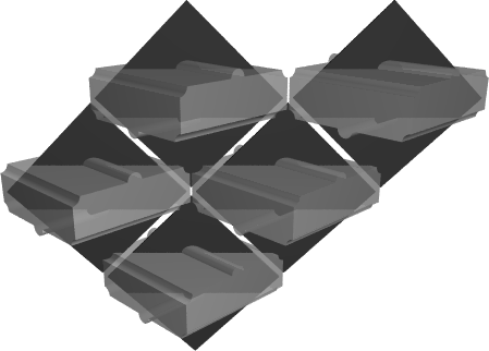
Proof.
Let us prove the first equation; the other three are similar. Note that the brick represented by the word is in position and thus lies in the th diagonal. Appending or to this word adds or to the position, which does not alter .
To see that the bricks of form a 2D Young diagram, observe that and commute in . The suffix corresponds to the box in the Young diagram. Again, the other cases are similar. The colours are easy to check directly. ∎
Figure 7 shows the central slice of the pyramid partition of Figure 5b. Every brick has been replaced with a square tile to make the orientation of the 2D Young diagram clear.
Lemma 5.9.
For , we have the following interlacing properties (where the prime denotes transposition of 2D Young diagrams):
Proof.
Let us handle the first case. Let be the set of bricks in the th column of , and suppose that . Explicitly,
In particular, each of the bricks in may be represented as some prefix of the word
Informally speaking, and form a chain of bricks, each of which rests on the previous one (see Figure 8). It follows from Definition 5.6 that ; then part (3) of Lemma 3.2 says that .

Next let us see that . Let be the th row of , with . We have
from which it follows that . This means that . See Figure 9 for an illustration of the difference between the row–interlacing and column–interlacing behaviour.
The remaining cases are similar. ∎


6. A generating function for pyramid partitions
We will now compute the following generating function for pyramid partitions.
Definition 6.1.
Let be a pyramid partition. For , let
denote the number of boxes coloured in . Define
Theorem 6.2.
where .
Theorem 6.2 may seem unrelated to the other theorems in this paper, but it will turn out that it is the key to computing . The proof is much like that of Theorem 1.4.
Proof.
We define a vertex operator product which counts pyramid partitions. Let us first define an operator which sweeps out four slices of the pyramid partition at the same time. Let
so that
It is simple to check this product against Lemmas 5.9 and 5.8 to be sure that it describes the correct colouring and interlacing behaviour. Set
Commuting the weight operators past the vertex operators gives
and
so that
| (7) |
The commutation relation for these operators is
Because of the mixed and operators, some of the commutation factors now appear in the numerator. We now move the operators in (7) to the left of the expression, while moving the operators to the right. As in the proof of Theorem 1.4, all of the vanish, and we are left with the commutator
where . ∎
Note that this method gives an alternate proof of the result in [32], when we specialize , .
7. Counting –coloured 3D Young diagrams
We will now prove Theorem 1.5. Let us name the elements of as in the previous section, and recall the definition of from Theorem 1.5. Our set of indeterminates is . Let .
Before we proceed to compute this generating function, consider the th diagonal slice of the positive octant. Note that we have
In particular, the box is coloured if , and otherwise. In other words, each diagonal slice of is now coloured in a checkerboard fashion, whereas in the case, they were single–coloured (see Figure 10). We need to introduce a two–coloured weight function if we are to use vertex operators to compute .


Definition 7.1.
For , let
We may write down a vertex operator product which sweeps out a 3D diagram in diagonal slices, according to the colouring. It is
| (8) |
Unfortunately, no longer commutes nicely with the operators, so our usual approach to computing with vertex operators fails here. The problem is fundamental, and it does not appear that we can resolve it in a natural way. We need a new idea.
However, there are two clues which tell us how to proceed. The first clue is that the desired formula for is very close to , so it would suffice to prove the following:
Lemma 7.2.
The second clue is that if we attempt to compute by slicing along lines , rather than , then the slices of the pyramid partition are checkerboard–coloured as well! See Figure 6, which shows the colouring scheme from below. The heavy black lines represent two edges of the pyramid, corresponding to prefixes of the words and , so bricks which lie on these lines represent the corners of the slices.
So, using our checkerboard coloured weight operators, we can write down a different vertex operator product which still counts pyramid partitions.
Lemma 7.3.
Proof.
Observe that (8) is very similar to the product in Lemma 7.3, so we shall look for a way to transform into .
Definition 7.4.
Define
Lemma 7.5.
The operators have the following properties:
In fact, unlike , also commutes nicely with the checkerboard weight operators .
Lemma 7.6.
Proof.
The operator has the effect of adding all possible border strips of length to the boundary of a 2D Young diagram. Since the length of the strips is even, any such has the same –weight. Indeed,
It follows that
and thus
The case of is similar. ∎
Finally, we have the following property of , inherited from the corresponding property of :
Proof of Lemma 7.2. Let us alter the first line of (8) by transforming half of the operators into operators,
Now, continue to move the term to the right through the second line of (8). We have
where is the product of the commutators generated by Lemma 7.5. Next, change half of the to in the above expression,
and commute them out to the left. This time, we pick up the multiplicative factor
and the factors cancel. We have shown that
8. Future work
It would obviously be wonderful to have a combinatorial proof of these identities; such a proof might be analagous to the “–quotient” on 2D Young diagrams, which decomposes a Young diagram into smaller Young diagrams and an –core. The authors suspect, however, that such a proof would be rather difficult to find. One indication of this is that there are formulae for 3D Young tableaux which fit inside an box, but computational evidence suggests that there is no such nice formula for –coloured partitions.
One could attempt to compute the Donaldson–Thomas partition functions of arbitrary toric Calabi-Yau orbifolds. To this aim, it should be possible to develop an orbifold version of the topological vertex formalism following [20]; this is a work in progress. It would also be interesting to try to extend Szendrői’s work [31] in noncommutative Donaldson–Thomas theory using the results of this paper.
One box counting problem which is of great interest is to take and the colouring given by
However, this problem appears to be rather difficult. The group representation does not naturally embed into or , so Donaldson–Thomas theory does not generate any conjectures as to what the answer might look like. Indeed, Kenyon [16] conjectures that there is no nice product formula in this example.
One unifying theme between 3D diagrams and pyramid partitions is quivers: both objects arise from a quiver path algebra modulo an ideal generated by a superpotential [31]. Perhaps one can extend the methods to other quivers and superpotentials.
However, the most intriguing direction for future work is simply to try to understand these proofs more fully. The reader may perhaps have noticed that the appearance of pyramid partitions seems somewhat unmotivated. Undoubtedly, there is some underlying geometric or representation-theoretic reason why these product formulae exist.
Appendix A Donaldson-Thomas theory of and its crepant resolution (by Dr. Jim Bryan)
A.1. Review of Donaldson-Thomas theory
Donaldson-Thomas theory, in its incarnation due Maulik, Okounkov, Nekrasov, and Pandharipande, constructs subtle integer valued deformation invariants of a threefold out of the Hilbert scheme of subschemes of . If is a Calabi-Yau threefold, i.e., is trivial, then this invariant has a simple formulation due to Behrend. It is given by the weighted topological Euler characteristic of the Hilbert scheme where the weighting is by , an integer valued constructible function which is canonically associated to any scheme [2].
Let be a (not necessarily compact) threefold with trivial canonical class. Let be the Hilbert scheme of subschemes having proper support of dimension less than or equal to one and with and . We define the Donaldson-Thomas invariant to be
where denotes topological Euler characteristic and is Behrend’s constructible function .
The invariants are assembled into the partition function as follows. Let be a basis for such that any effective curve class is given by with . Let be corresponding variables and let . The Donaldson-Thomas partition function of is defined by
Define the reduced partition function by
where the second equality is a theorem proved by [3, 17, 18].
Maulik, Nekrasov, Okounkov, and Pandharipande conjecture that Donaldson-Thomas theory is equivalent to Gromov-Witten theory. We assemble , the genus Gromov-Witten invariants of non-zero degree into the reduced Gromov-Witten partition function as follows:
Conjecture A.1.
[21] Under the change of variables the reduced partition functions of Donaldson-Thomas and Gromov-Witten theory are equal:
A.2. Orbifold Donaldson-Thomas theory of
Extending Donaldson-Thomas theory to the case of three dimensional orbifolds is expected to be routine since the Hilbert scheme of substacks of a Deligne-Mumford stack has been constructed by Olsson and Starr [28], although it isn’t clear how best to choose the discrete data in general.
The orbifolds that we consider are simple enough that we can identify the Hilbert scheme directly. Let be a finite subgroup of . A substack of may be regarded as a -invariant subscheme of , and consequently we can regard the Hilbert scheme of as a subset of the Hilbert scheme of . Since we require our substacks to have proper support, we need only consider zero dimensional subschemes of . For any -representation of dimension we identify as follows:
This Hilbert scheme has a symmetric perfect obstruction theory induced by the -invariant part of the of the perfect obstruction theory on . However, we do not need this construction since we can define the Donaldson-Thomas invariants directly using Behrend’s constructible function.
Definition A.2.
The Donaldson-Thomas invariants of are indexed by representations of and are given by the Euler characteristics of the Hilbert schemes, weighted by Behrend’s function:
Let be variables corresponding to , the irreducible representations of . For a representation , let denote . We define the orbifold Donaldson-Thomas partition function by
where runs over all representations of .
We now restrict our attention to groups which are subgroups of and are Abelian. Finite subgroups of admit an ADE classification. They are the cyclic groups, the dihedral groups, and the platonic groups. The only Abelian groups from this list are the cyclic groups and the Klein 4-group . The action of on is given by
where . The action of on is given by
As in the introduction, we choose an isomorphism of the group of representations with . Explicitly, we identify with , the representation of where acts by multiplication by . For we identify , and with the representations , , and given by the action on the , , and coordinates of respectively.
Theorem A.3.
Let be the variable corresponding to the group element and the character . Then
where is the -coloured 3D diagram partition function introduced and computed in the main body of the paper (Theorem 1.4).
Let be variables corresponding to , the group elements of , and , the characters of . Then
where is the -coloured 3D diagram partition function introduced and computed in the main body of the paper (Theorem 1.5).
Proof: Let be or and let be the subtorus with . The action of on commutes with the action of and hence defines a -action on and on . The fixed points of in are isolated, even infinitesimally [3, Lemma 4.1], and they correspond to monomial ideals in . The monomial ideals in turn correspond to 3D Young diagrams where if denotes the -fixed subscheme of , then
as a -representation viewed as a polynomial in modulo the relation . Following [21], we adopt the notation
By [3, Prop. 3.3], the -weighted Euler characteristic of is given by a sum over the -fixed points, counted with sign given by the parity of the dimension of the Zariski tangent space of at a fixed point corresponding to 3D diagram . Hence both the Donaldson-Thomas and the diagram partition functions are given by a sum over 3D diagrams, weighted, up to a sign, by the same variables. Thus our main task is to determine the sign.
Let be a 3D diagram having boxes and having boxes of colour . Let denote the Zariski tangent space of at the subscheme corresponding to . Let
be the Zariski tangent space of at the same point. can be regarded as both a -representation and a -representation. is given by the -invariant subspace of .
The difference of and its dual , regarded as a virtual -representation, is computed in [21, equation (13)] and given by
where
Using the relation to eliminate from the above expression, we can regard as an element in
the virtual representation ring of .
Following [21], we let
which satisfies the easily verified equation
| (9) |
in , and also has the crucial property that the constant term of is even [21, Lemma 10]. These facts allow us to use as a surrogate for when computing the parity of the dimension:
Lemma A.4.
Let and denote the -invariant part of and respectively, then
Proof: From equation (9) we see that is self-dual. Thus all non-constant monomials occur in pairs of the form . Moreover, the constant term of is even [21, Lemma 10] and the constant term of is zero [3, Lemma 4.1]. Thus we have
Indeed, the above argument shows that if we restrict to any self-dual collection of weights, the virtual dimension will be even. In particular, the -invariant part of has even virtual dimension, which proves the lemma. ∎
To compute the parity of the -invariant part of , we work in the representation ring of with mod 2 coefficients. The restriction map
is explicitly given by
in the case where , and by
in the case where .
For any and any irreducible representation , let denote the coefficient of in . We compute in
as follows.
Since is equal to the dimension of the -invariant part of modulo 2, the 3D diagram is counted with sign in the Donaldson-Thomas partition function of . This proves first part of Theorem A.3.
We now compute in
We use the fact that in this ring, the square of an arbitrary element is equal to the sum of its coefficients:
and we compute as follows.
Since is equal to the dimension of the -invariant part of modulo 2, the 3D diagram is counted with sign in the Donaldson-Thomas partition function of . This proves the remaining part of Theorem A.3 and so the proof of Theorem is complete.∎
Remark A.5.
For any finite Abelian subgroup , the Donaldson-Thomas invariants of are given by a signed count of boxes coloured by . However, it is not always true that this sign is obtained by simply changing the signs of some of the variables. For example, consider the case of acting on with equal weights on all three factors. The sign associated to a 3D partition can be computed by the methods of this appendix and is given by , where
Thus the coloured 3D diagram partition function and the Donaldson-Thomas partition function are not related in an obvious way.
A.3. The Donaldson-Thomas crepant resolution conjecture
A well known principle in physics asserts that string theory on a Calabi-Yau orbifold is equivalent to string theory on any crepant resolution . Consequently, it is expected that mathematical counterparts of string theory, such as Gromov-Witten theory or Donaldson-Thomas theory, should be equivalent on and . Precise formulations of these equivalences are known as crepant resolution conjectures. The crepant resolution conjecture in Gromov-Witten theory goes back to Ruan, and has recently undergone successive refinements [29, 8, 11, 12].
In this section we formulate a crepant resolution conjecture for Donaldson-Thomas theory. Our conjecture has somewhat limited scope: we stick to the “local case” where is of the form , and (for reasons explained below) we impose the hard Lefschetz condition [8, Defn 1.1], which implies [7] that is a finite subgroup of either or .
The most straightforward formulation of the crepant resolution conjecture in Donaldson-Thomas theory posits that the partition functions of the orbifold and its resolution are equal after some natural change of variables. For the orbifold , we saw in the previous section that the partition function has variables naturally indexed by irreducible -representations. By the classical McKay correspondence, the crepant resolution given by the -Hilbert scheme has a basis of also labelled by irreducible -representations [6, 22]. However, the variables of the Donaldson-Thomas partition function of correspond to a basis of . So in order to get the number of variables of and to match, we need
This occurs if and only if is a semi-small resolution. This condition is equivalent to the orbifold satisfying the hard Lefschetz condition.
Conjecture A.6.
Let be a local, 3 dimensional, Calabi-Yau orbifold satisfying the hard Lefschetz condition, namely, where is a finite subgroup of either or .
Let be variables corresponding to the irreducible -representations where is the trivial representation. Let be the crepant resolution given by the -Hilbert scheme and let be the variables corresponding to the basis of curve classes in labelled by the non-trivial -representations .
Then the Donaldson-Thomas partition functions of and are related by the formula
under the identification of the variables
Proposition A.7.
Conjecture A.6 holds for Abelian, namely for or .
Remark A.8.
Szendrői proved [31] that a similar relationship holds between the Donaldson-Thomas partition functions of the non-commutative conifold singularity and its small resolution.
Remark A.9.
The Gromov-Witten partition function of has been computed for all in or in [7] (see also Remark A.10). This provides, via the MNOP conjecture, a prediction for and hence our conjecture A.6 gives a prediction for which can be tested term by term. Verification of this prediction for terms of low order has been obtained by D. Steinberg in the case where is the quaternion 8 group.
In light of Theorems 1.4, 1.5, and A.3, Proposition A.7 is equivalent to Theorem 1.7 which we prove here.
A.3.1. Proof of Proposition A.7 / Theorem 1.7:
Since is Abelian, is toric and so via [21, Theorems 2 and 3], the reduced Donaldson-Thomas partition function of is equal to the reduced Gromov-Witten partition function of after the change of variables . Thus it suffices to compute the Gromov-Witten partition function of 11 1 In [21] it is shown that the reduced Donaldson-Thomas partition function of a toric Calabi-Yau threefold can be computed via the topological vertex formalism. In general, the topological vertex formalism has been proven to compute the Gromov-Witten partition function only in the “two-leg” case. While is a local surface and can be computed with two-leg vertices, has the geometry of the closed topological vertex [9] and requires a three-leg vertex. However, in this case, the invariants have been computed by both the vertex formalism as well as by localization and have been shown to agree [15]. Thus we know that the Gromov-Witten/Donaldson-Thomas correspondence holds for both and .. The pithiest way to encode the Gromov-Witten invariants is in terms of Gopakumar-Vafa invariants, or so called BPS state counts. It is well know that each genus zero BPS state count contributes a factor of to the Gromov-Witten partition function (see for example the proof of Theorem 3.1 in [4]). Thus the content of Theorem 1.7 is that has genus 0 Gopakumar-Vafa invariants occurring in the classes for with value -1, and that has genus 0 Gopakumar-Vafa invariants occurring in the classes , , , and with value 1 and in the classes , , and with value -1. Moreover, all other Gopakumar-Vafa invariants are zero. These assertions are proved in [15]: the case of is Corollary 16 and Proposition 19 and the case of is Proposition 12. ∎
Remark A.10.
The Gromov-Witten and Donaldson-Thomas theories of are equivariant theories and so in general depend on the choice of the torus action. In this paper, we have assumed that the torus is chosen to act trivially on the canonical class. This choice is required to apply the topological vertex formalism as we have done in the above proof. We warn the reader that the computation of the Gromov-Witten invariants of for general done in [7] is done using the action induced from the diagonal action on . This does not change which classes carry Gopakumar-Vafa invariants, but it can change the values of the invariants in those curve classes that admit deformations to infinity.
References
- [1] George G. Andrews and Peter Paule, MacMahon’s dream, Preprint, http://www.math.psu.edu/andrews/preprints.html.
- [2] K. Behrend, Donaldson-Thomas type invariants via microlocal geometry, ArXiv: math.AG/0507523.
- [3] K. Behrend and B. Fantechi, Symmetric obstruction theories and Hilbert schemes of points on threefolds, ArXiv: math.AG/0512556.
- [4] Kai Behrend and Jim Bryan, Super-rigid Donaldson-Thomas invariants, Mathematical Research Letters 14 (2007), no. 4, 559–571, arXiv version: math.AG/0601203.
- [5] David M. Bressoud, Proofs and confirmations: the story of the alternating sign matrix conjecture, Cambridge University Press, Cambridge, 1999.
- [6] Tom Bridgeland, Alastair King, and Miles Reid, The McKay correspondence as an equivalence of derived categories, J. Amer. Math. Soc. 14 (2001), no. 3, 535–554 (electronic). MR MR1824990 (2002f:14023)
- [7] Jim Bryan and Amin Gholampour, The Quantum McKay correspondence for polyhedral singularities, In preparation.
- [8] Jim Bryan and Tom Graber, The crepant resolution conjecture, To appear in Algebraic Geometry — Seattle 2005 Proceedings, arXiv: math.AG/0610129.
- [9] Jim Bryan and Dagan Karp, The closed topological vertex via the Cremona transform, Journal of Algebraic Geometry 14 (2005), 529–542, arXiv version math.AG/0311208.
- [10] Jim Bryan and Rahul Pandharipande, The local Gromov-Witten theory of curves, J. Amer. Math. Soc. 21 (2008), no. 1, 101–136 (electronic), With an appendix by Bryan, C. Faber, A. Okounkov and Pandharipande. MR MR2350052
- [11] Tom Coates, Alessio Corti, Hiroshi Iritani, and Hsian-Hua Tseng, Wall-Crossings in Toric Gromov-Witten Theory I: Crepant Examples, arXiv:math.AG/0611550.
- [12] Tom Coates and Yongbin Ruan, Quantum Cohomology and Crepant Resolutions: A Conjecture, arXiv:0710.5901.
- [13] William Fulton and Joe Harris, Representation theory: A first course, Springer-Verlag New York, Inc., 175 Fifth Ave., New York NY, 10010, USA, 1991.
- [14] Emden R. Gansner, The enumeration of plane partitions via the Burge correspondence, Illinois J. Math 25 (1981), no. 2, 533–554.
- [15] Dagan Karp, Chiu-Chu Melissa Liu, and Marcos Marino, The local Gromov-Witten invariants of configurations of rational curves, arXiv:math.AG/0506488.
- [16] Richard Kenyon, Talk at the workshop on random partitions and Calabi-Yau crystals, Amsterdam, 2005. Available at http://www.math.brown.edu/rkenyon/talks/pyramids.pdf.
- [17] M. Levine and R. Pandharipande, Algebraic cobordism revisited, arXiv:math/0605196.
- [18] Jun Li, Zero dimensional Donaldson-Thomas invariants of threefolds, Geom. Topol. 10 (2006), 2117–2171 (electronic). MR MR2284053 (2007k:14116)
- [19] Percy A. MacMahon, Combinatory analysis, Cambridge University Press, The Edinburgh Building, Cambridge, UK, 1915-16.
- [20] D. Maulik, N. Nekrasov, A. Okounkov, and R. Pandharipande, Gromov-Witten Theory and Donaldson-Thomas Theory, Compos. Math 142 (2006), no. 5, 1263–1304.
- [21] D. Maulik, N. Nekrasov, A. Okounkov, and R. Pandharipande, Gromov-Witten theory and Donaldson-Thomas theory. I, Compos. Math. 142 (2006), no. 5, 1263–1285. MR MR2264664 (2007i:14061)
- [22] John McKay, Graphs, singularities, and finite groups, The Santa Cruz Conference on Finite Groups (Univ. California, Santa Cruz, Calif., 1979), Proc. Sympos. Pure Math., vol. 37, Amer. Math. Soc., Providence, R.I., 1980, pp. 183–186. MR MR604577 (82e:20014)
- [23] A. Okounkov and R. Pandharipande, The local Donaldson-Thomas theory of curves, arXiv:math.AG/0512573.
- [24] Andrei Okounkov, Infinite wedge and random partitions, Selecta Math. (N.S.) 7 (2001), no. 1, 57–81.
- [25] Andrei Okounkov and Nikolai Reshetikhin, Correlation function of Schur process with application to local geometry of a random 3-dimensional Young diagram, J. Amer. Math. Soc. 16 (2003), no. 3, 581–603.
- [26] by same author, Random skew plane partitions and the pearcey process, Communications in Mathematical Physics 269 (2007), no. 3, 571–609.
- [27] Andrei Okounkov, Nikolai Reshetikhin, and Cumrun Vafa, Quantum Calabi-Yau and classical crystals, Progress in Mathematics 244 (2006), 597–618.
- [28] Martin Olsson and Jason Starr, Quot functors for Deligne-Mumford stacks, Comm. Algebra 31 (2003), no. 8, 4069–4096, Special issue in honor of Steven L. Kleiman. MR MR2007396 (2004i:14002)
- [29] Yongbin Ruan, The cohomology ring of crepant resolutions of orbifolds, Gromov-Witten theory of spin curves and orbifolds, Contemp. Math., vol. 403, Amer. Math. Soc., Providence, RI, 2006, pp. 117–126. MR MR2234886
- [30] Richard P. Stanley, Enumerative combinatorics, vol. 2, Cambridge University Press, The Edinburgh Building, Cambridge, UK, 2001.
- [31] Balázs Szendrői, Non-commutative Donaldson-Thomas theory and the conifold, To appear in Geometry and Topology. arXiv:0705.3419v1 [math.AG].
- [32] Benjamin J. Young, Computing a pyramid partition generating function with dimer shuffling, Preprint: arXiv:0709.3079.