Joint Source Channel Coding with Side Information Using Hybrid Digital Analog CodesThanks: This work was supported by the National Science Foundation under grant CCR 0515296.
Abstract
We study the joint source channel coding problem of transmitting an analog source over a Gaussian channel in two cases - (i) the presence of interference known only to the transmitter and (ii) in the presence of side information known only to the receiver. We introduce hybrid digital analog forms of the Costa and Wyner-Ziv coding schemes. Our schemes are based on random coding arguments and are different from the nested lattice schemes by Kochman and Zamir that use dithered quantization. We also discuss superimposed digital and analog schemes for the above problems which show that there are infinitely many schemes for achieving the optimal distortion for these problems. This provides an extension of the schemes by Bross et al to the interference/side information case. We then discuss applications of the hybrid digital analog schemes for transmitting under a channel signal-to-noise ratio mismatch and for broadcasting a Gaussian source with bandwidth compression.
I Introduction and Problem Statement
Consider the classical problem of transmitting samples of a discrete-time independent identically distributed (i.i.d) real Gaussian source in uses of an additive white Gaussian noise (AWGN) channel such that the mean-squared error distortion is minimized. Let the source be encoded into the sequence which satisfies a power constraint . Let us first consider the case of and let the output of the AWGN channel be given by
where is a noise vector of i.i.d Gaussian random variables with zero mean and variance . If the source variance is , then the optimal mean-squared error distortion that can be achieved is . This optimal performance can be achieved by two very simple schemes. The first one is separate source and channel coding, where the source is first quantized and the quantization index is transmitted using an optimal code for the AWGN channel. The second scheme is uncoded (analog) transmission with power scaling [4, 5], where the source is not explicitly quantized. Recently, it was shown by Bross, Lapidoth and Tinguely [7] that there is a family of infinitely many schemes that are optimal, which contains the separation based scheme and uncoded (analog) transmission as special cases.
In this paper, we consider the problem of transmitting samples of an i.i.d Gaussian source through uses of an AWGN channel. We will refer to the ratio of as the bandwidth efficiency . We first consider the case of and the presence of an interference known only to the transmitter and/or side information available only at the receiver. We derive hybrid digital analog (HDA) coding schemes for these cases where the source is not explicitly quantized and show that they can obtain the optimal distortion. These can be viewed as the equivalent of uncoded transmission but in the presence of an interference or side information. Then, we show that there is a family of infinitely many schemes that are optimal for this problem which contain pure separation based schemes and HDA schemes as special cases. This can be viewed as the extension of Bross, Lapidoth and Tinguely’s [7] result in the presence of interference/side-information. An interesting aspect of the hybrid digital analog coding schemes proposed here is that they do not require binning unlike their separation based counterparts.
The HDA scheme proposed here for the case of interference known at the transmitter is closely related to the scheme considered by Kochman and Zamir in [8], although this was developed independently. The difference is that the proposed scheme is based only on random coding arguments and does not use nested lattices like in [8]. As a result, the relationship between the auxiliary random variable and the source is made more explicit. We also consider several applications of the HDA schemes which are not considered in [8]. We consider the non-asymptotic SNR case unlike in [8]. Further, the performance of this scheme in the presence of SNR mismatch is analyzed. Finally, the use of a HDA Costa based scheme for broadcasting a Gaussian source to two users with bandwidth compression, where is discussed. In the case of side-information available only at the receiver, the proposed scheme is similar to the scheme in [3] and again uses random coding arguments instead of nested lattices.
The paper is organized as follows. First in Section II, we discuss the problem of transmitting an i.i.d Gaussian source in the presence of a Gaussian interference known only to the transmitter. We introduce a hybrid digital analog (HDA) Costa coding scheme where the source is not explicitly quantized and show that this is optimal. We then discuss a generalized HDA Costa coding scheme and show that there infinitely many schemes that are optimal. In Section III, we discuss similar schemes and results for the case of having side information available only at the receiver (Wyner-Ziv problem) and in Section IV, briefly consider the situation having interference known only to the transmitter and side-information available only at the receiver. In [12], Merhav and Shamai have shown that separate Wyner-Ziv coding followed by Gelfand-Pinsker coding is optimal for this problem. However, we show that there is a joint source-channel coding scheme for the case of Gaussian source, interference and side information. This result in Section IV is a fairly straightforward extension of the results in Section II and Section III, but is included for completeness and to make the exposition clear. In Section V, we study the performance of these schemes when the SNR of the channel is different from the designed SNR and in Section VI the distortion exponents of these schemes are analyzed. In Section VII, we consider the problem of transmitting a Gaussian source in the absence of an interference, but when the channel bandwidth is smaller than the source bandwidth and show how the HDA Costa coding scheme is useful. Finally, in Section VIII, we consider the problem of broadcasting a Gaussian source to two users through AWGN channels and propose a joint source channel coding scheme based on HDA Costa coding.
We use the following notation in this paper. Vectors are denoted by bold face letters such as . Upper case letters are used to denote scalar random variables. When considering a sequence of i.i.d random variables, a single upper case letter is used to denote each component of the random vector.
II Transmission of a Gaussian source over a Gaussian channel with interference known only at the transmitter
We first consider the problem of transmitting samples of a real analog source (this corresponds to ) , with components which are independent Gaussian random variables with in uses of an AWGN channel with noise variance in the presence of an interference which is known to the transmitter but unknown to the receiver. Further, let us assume that ’s are a sequence of real i.i.d Gaussian random variables with zero mean and variance and let the input power to the channel be constrained to be . The problem setup is shown schematically in Fig. 1. The received signal is given by
| (1) |
where is the interference and is the AWGN.
The optimal distortion of can be obtained even in the presence of the interference by using the following (obvious) separate source and channel coding scheme.
II-A Separation based scheme with Costa coding (Digital Costa Coding)
We first quantize the source using an optimal quantizer to produce an index , where . Then, the index is transmitted using Costa’s writing on dirty paper coding scheme [10]. Since the quantizer output is digital information, we refer to this scheme as digital Costa coding. We briefly review this here to make it easier to describe our proposed techniques later on.
Let be an auxiliary random variable given by
| (2) |
where is independent of and .
We first create an -length i.i.d Gaussian code book with codewords, where each component of the codeword is Gaussian with zero mean and variance . Then evenly (randomly) distribute these over bins. For each , let be the index of the bin containing . For a given , we look for an such that and are jointly typical. Then, we transmit . Note that since are jointly typical, from (2), we can see that and satisfies the power constraint.
The received sequence is given by
| (3) |
At the decoder, we look for a that is jointly typical with and declare to be the decoded message. Since , the distortion in given by , where is the distortion rate function. For a Gaussian source and mean squared error distortion and, hence, the overall distortion can be made to be arbitrarily close to by a proper choice of and .
While the above scheme is straightforward, in the following three sections we show that there are a few other joint source channel coding schemes, which are also optimal. In fact, there are infinitely many schemes which are optimal. Although, these schemes are all optimal when the channel SNR is known at the transmitter, their performance is in general different when there is an SNR mismatch. The joint source channel coding schemes to be discussed in the next sections have advantages over the separation based scheme discussed in such a situation.
II-B Hybrid Digital Analog Costa Coding
Let us now describe a joint source-channel coding scheme where the source is not explicitly quantized. We refer to this scheme as hybrid digital analog (HDA) Costa coding for which the code construction, encoding and decoding procedures are as follows.
We first define an auxiliary random variable given by
| (4) |
where and , and are pairwise independent.
- 1.
Codebook generation: Generate a random i.i.d code book with sequences, where each component of each codeword is Gaussian with zero mean and variance .
- 2.
Encoding: Given an and , find a such that are jointly typical with respect to the distribution obtained from the model in (4) and transmit . If such an cannot be found, we declare an encoder failure. Let be the probability of an encoder failure.
From standard arguments on typicality and its extensions to the infinite alphabet case [16], it follows that as provided
(5) (6) (7) (8) (9) where the results follow because and . Notice that when a that is jointly typical with and is found, satisfies the power constraint.
- 3.
Decoding : The received signal is . At the decoder, we look for an that is jointly typical with . If such a unique can be found, we declare as the decoder output or, else, we declare a decoder failure. Let be the probability of the event that the decoder output is not equal to the encoded (this includes the probability of decoder failure as well as the probability of a decoder error).
In order to analyze , consider the equivalent communication channel between and . Notice that we have in effect transmitted a codeword from a random i.i.d codebook for with codewords through the equivalent channel whose output is . Again, from the extension of joint typicality to the infinite alphabet case, as provided that
(10) Now, let us choose
(11) (12) For the above choice of , it can be seen that
and, hence, (10) reduces to
(13) Hence, can be made arbitrarily small as long as
(14) Combining this with the condition for encoder failure, and can both be made arbitrarily small provided
(15) Therefore, by choosing an , and we can satisfy (15) and make and as .
- 4.
Estimation: If there is no decoding failure, we form the final estimate of as an MMSE estimate of from . After some algebra this is given by ,
(16) The distortion is then given by,
(17) with is vanishing for arbitrarily small . If an encoder or decoder failure was declared, we set the estimate of to be the zero vector. However, as shown above the probability of these events can be made arbitrarily small and, hence, they do not contribute to the overall distortion, which can be seen to be arbitrarily close to the optimal distortion achievable in the absence of the interference.
We have presented a joint source channel coding scheme in the presence of an interference known only to the transmitter. The use of the term hybrid digital analog Costa coding needs some explanation. The scheme is not entirely analog in that the auxiliary random variable is from a discrete codebook. However, in contrast to digital Costa coding, the source is not explicitly quantized and is embedded into the transmitted signal in an analog fashion. This is the reason for calling this as HDA Costa coding and this has some interesting consequences which are discussed in the following section.
Another feature of the HDA Costa coding scheme is that it does not make use of binning, rather it needs a single quantizer codebook that is also a good channel code. In practice, this may have some impact on the design since there are ensembles of codes that are provably good quantizers and channel codes [14]. In the Gaussian case, good lattices that are both good for coding and for quantization are known. The binning approach however, requires a nesting condition. That is, the fine code much be a good channel code, but it much contain a subcode (or a coarse code) and its cosets that must be good quantizers. This may be a more difficult condition to obtain in practice.
II-C Superimposed digital and HDA Costa coding scheme
Recently in [7], Bross, Lapidoth and Tinguely considered the problem of transmitting samples of a Gaussian source in uses of an AWGN channel, in the absence of the interferer. They showed that there are infinitely many superposition based schemes, which contain pure separation based scheme and uncoded transmission as special cases. In this section, we show that the same is true in the presence of an interference also and show the corresponding scheme, which is given in Fig. 2.
The transmitted signal is a superposition of two signals and , which are the outputs of a digital Costa encoder and an HDA encoder, respectively.
The source is first quantized at a rate of using an optimal source code and let the quantization error be , where is the reconstruction. The quantization error has a variance . The first stream in Fig. 2 is a digital Costa encoder that encodes the quantization index by treating as interference and produces the signal , which has a power of . The second stream is a HDA Costa encoder of rate which treats and as interference and produces , which has a power of . The transmitted signal is the superposition (sum) of and .
In the digital Costa encoder in the first stream, the auxiliary random variable is given by with . A power of is used in the first stream and is chosen as . Note that this corresponds to treating as noise in addition to the channel noise.
In the second stream, the quantization error is encoded using an HDA Costa coding scheme and a power of is used. Note that since , the power is always positive. The auxiliary random variable is chosen as , where acts as the net interference. Hence, is chosen to be independent of , and , and is chosen to be . is chosen similar to (12) which gives .
At the decoder the quantization index from the first stream is first decoded and the reconstruction is obtained. Then, an estimate of the quantization error is obtained from the second stream using the HDA costa decoder. The overall distortion is the distortion in estimating . Using the analysis of the HDA Costa scheme in Section II-B, this can be seen to be
| (18) |
By choosing to be arbitrarily small we can make and achievable a distortion of , which is the optimal distortion.
Note that for any source coding rate chosen in the first stream namely , the resulting distortion is optimal. By varying , we can get an infinite family of optimal joint source channel coding schemes.
II-D Generalized Hybrid Costa coding
In the previous section, we described a superposition technique. In this section we show a scheme that does not explicitly do superposition. Moreover this also introduces an interesting scheme that is intermediate between HDA Costa having no bins to the digital Costa having bins corresponding to the capacity of the channel.
Once again we quantize the source to at a rate , that is strictly lesser than the channel capacity, using an optimal vector quantizer. Let be the quantization error vector. Note that for an optimal quantizer, as the Rate-Distortion limit is approached, the quantization error will be Gaussian.
We next define an auxiliary random variable given by
| (19) |
where , and , and are independent of each other. and are constants, the choice of which is discussed below
- 1.
Codebook generation: Generate a random i.i.d code book with sequences, where each component of each codeword is Gaussian with zero mean and variance . These codewords are uniformly distributed in bins and this is shared between the encoder and the decoder.
- 2.
Encoding: Let be the quantization index corresponding to the quantized source . Let represent the index of a bin that contains . For a given find an such that and are jointly typical with respect to the distribution in model (19). We next transmit the vector . Note that since are jointly typical, from (19), we can see that and satisfies the power constraint.
- 3.
Decoding : The received signal is . At the decoder, we look for an that is jointly typical with . If such a unique can be found, we declare as the decoder output or, else, we declare a decoder failure. Next we make an estimate of from and .
We can see by similar Gelfand-Pinsker coding arguments that . Note
(20) In (20) we choose and . The choice of ensures is orthogonal to to get the equality in (a). is chosen as above to satisfy the inequality in (b). This shows that we can decode the codeword with a very high probability and we can decode the message and .
- 4.
Estimation: If there is no decoding failure, we form the final estimate of as an MMSE estimate of from . The estimate can be obtained as follows. Let us define . Let be the covariance matrix of and let be the correlation vector between and . Then, and are given by
.
The coefficients of the linear MMSE estimate are given by and the minimum mean-squared error is given by
where as . Thus, in the limit of , .
It must be noted that this scheme is an intermediate between digital Costa coding scheme with the maximum possible bins equal to the capacity of the channel and the analog Costa coding scheme with no bins. Thus we can get a family of schemes with varying bins for the Gaussian channel.
The generalized hybrid Costa coding scheme appears to be closely related to the superimposed digital and HDA Costa coding schemes. The subtle difference however is in the generalized hybrid Costa coding scheme, the transmitted signal is not a superposition of two streams as seen in the superposition case.
III Transmission of a Gaussian source through a channel with side information available only at the receiver
In this section we consider the problem of transmitting a discrete-time analog source over a Gaussian noise channel when the receiver has some side information about the source. This problem is a dual of the problem considered in the previous section and is considered here for the sake of completeness. Consider the system model as follows. Let be the discrete-time analog source where ’s are independent Gaussian random variables with . Let be the side information that is known only at the receiver. The correlation between the source and the side information is modeled as
| (21) |
where and is i.i.d Gaussian. Here and are mutually independent random variables. The source must be encoded into and transmitted over an AWGN channel and the received signal is
| (22) |
where satisfies a power constraint and is AWGN having a noise variance of . The following schemes can be shown to be optimal for this case.
III-A Separation Based Scheme with Wyner Ziv Coding (Digital Wyner Ziv Coding)
One strategy is using a separation scheme with an optimal Wyner-Ziv code of rate followed by a channel code. We also refer to this scheme as the digital Wyner-Ziv scheme. We briefly explain the digital Wyner-Ziv scheme and then establish our information theoretic model for the HDA Wyner-Ziv coding scheme.
Suppose the side information is available both at the encoder as well as the receiver, the best possible distortion is . The same distortion can be achieved using the following scheme and is a direct consequence of Wyner and Ziv’s result [17]. This can be achieved as follows,
Let be an auxiliary random variable given by
| (23) |
where and . We create an -length i.i.d Gaussian code book with codewords, where each component of the codeword is Gaussian with zero mean and variance and evenly distribute them over bins. Let be the index of the bin containing . For each , find an such that are jointly typical. The index is the Wyner-Ziv source coded index. The index is encoded using an optimal channel code of rate arbitrarily close to and transmitted over the channel. At the receiver decoding of the index is possible with high probability as an optimal code book for the channel is used. Next for the decoded we look for an in the bin whose index is such that are jointly typical. From and the decoded we make an estimate of the source as follows.
| (24) |
This yields the optimal distortion D.
III-B Hybrid Digital Analog Wyner Ziv Coding
In this section, we discuss a different joint source channel coding scheme that does not involve quantizing the source explicitly. This scheme is quite similar to the modulo lattice modulation scheme in [3]; the difference being that a nested lattice is not used. The auxiliary random variable is generated as follows.
| (25) |
where is defined as and .
- 1.
Codebook generation: Generate a random i.i.d code book with sequences, where each component of each codeword is Gaussian with zero mean and variance . This codebook is shared between the encoder and the decoder.
- 2.
Encoding: For a given find an such that are jointly typical and transmit . This is possible with arbitrarily high probability if
- 3.
Decoding: The received signal is . Find an such that are jointly typical. A unique such can be found with arbitrarily high probability if . We next show below that we can choose an to satisfy . This requires which can be shown as follows
(26) In (26), (a) follows because is independent of and . (b) follows because we can always find a for the choice of . Hence from knowing , and we can make an estimate of . Since all random variables are Gaussian, the optimal estimate is a linear MMSE estimate which can be computed as follows.
Let be the covariance matrix of and let be the correlation between and . and are given by
.
The coefficients of the linear MMSE estimate are given by and this yields the optimal MMSE estimate which is given below as,
(27) The distortion is given by
Here, (a) follows by using the appropriate values of and . We once again obtain the optimal distortion by making arbitrarily small and .
It is instructive to compare the performance of this scheme with that of the following naive scheme that would be optimal in the absence of side-information at the receiver. In the naive scheme, the is transmitted directly (analog transmission). At the receiver, an MMSE estimate of is formed from the received signal and the available side information . The distortion for this naive scheme can be seen to be .
Notice that , whereas for the Wyner-Ziv scheme, . At , both and are zero. i.e. the optimal scheme and the naive scheme approach zero distortion with different slopes.
III-C Superimposed digital and HDA Wyner-Ziv scheme
The above results could also be extended to a form of superimposed digital and analog coding. This is similar to the superimposed digital and HDA Costa coding case discussed in section II-C. We once again have two streams as shown in Fig 4. The first stream uses a rate Wyner Ziv code to quantize the source assuming the side information is known at the receiver and the discrete index is encoded using an optimal channel code to produce the codeword . The power allocated to this stream is . The second stream uses the HDA Wyner-Ziv scheme and produces the output . The auxiliary random variable of the HDA scheme is given by
| (29) |
with , where and and are independent. We also choose where .
The two streams ( and ) are superimposed and transmitted through the channel. The received signal is given by . At the receiver is decoded assuming as independent noise and this gives the Wyner-Ziv encoded bits (index). This along with the side information can be used to make an estimate of the source and we call the estimate as . The random variables corresponding to and are related as
| (30) |
with having a variance . When the digital part is first decoded and canceled from the received signal, we get an equivalent channel for the HDA Wyner-Ziv scheme with power constraint and channel noise . We next make a final estimate of using a HDA Wyner-Ziv decoder from the new side information , the observed equivalent channel and the decoded . Notice that since the choice of where is designed for the side information , this ensures decoding of with arbitrarily high probability. The achievable distortion is then given as follows.
Here in (III-C) (a) follows since we assume that the first stream is decoded with high probability and apply the results of HDA Wyner-Ziv decoding with the side information . Also (b) follows since . The optimal distortion can be obtained by making arbitrarily small and . Notice that for any rate , , where is the capacity of the AWGN channel, there is a corresponding power allocation for for which the overall scheme is optimal. Thus, there are infinitely many schemes which are optimal with the digital Wyner-Ziv corresponding to and the HDA Wyner-Ziv corresponding to and .
Further, we would like to mention that there is another way to get a family of optimal schemes using the HDA Wyner-Ziv scheme. Here, the source is encoded using a HDA Wyner-Ziv encoder to the sequence . The auxiliary random variable is given by
| (32) |
where . The sequence can be treated as an i.i.d Gaussian source and, hence, the family of schemes proposed by Bross, Lapidoth and Tinguely [7] can be applied on . The scheme proposed in [7] quantizes the analog source, which in this case is to a quantization index and is sent over the Gaussian channel along with the uncoded analog source (here ) with the appropriate power scaling. At the receiver we can obtain an optimal estimate of by first decoding the quantized index and then making an estimate on the analog source. Notice that the HDA Wyner-Ziv receiver only requires an optimal MMSE estimate of , which can be obtained using the family of schemes in [7]. Hence the resulting distortion in is still optimal. To establish this claim we need to show that can be decoded with arbitrarily high probability and an optimal estimate of must be made using and the MMSE estimate .
We next show below that . Hence, we can choose a codebook for with codewords such that . Since , we can find a that is jointly typical with with probability close to 1 and since , can decoded with high probability from .
| (33) | |||||
In (33), (a) follows because is orthogonal to and hence is independent of and , (b) follows because is Gaussian with variance and is orthogonal to . The estimate of is then given by
| (34) |
The resulting distortion can be obtained by following the steps similar to those in (3) which can be found to be optimal.
IV Transmission of a Gaussian Source with Interference at the Transmitter and Side Information at the Receiver
In this section, we consider the problem of transmitting a Gaussian source through an AWGN channel with channel noise variance in the presence of an interference known only at the transmitter and in the presence of side information known only at the receiver. The side information is assumed to be related to the source according to
where and is independent of .
A similar model has been considered by Merhav and Shamai [12] for a more general setup where the source and side information are not assumed to be Gaussian. They show that a separation based approach of Wyner-Ziv coding followed by Gelfand-Pinsker coding is optimal. Here, we propose a joint-source channel coding scheme when the source and channel noise are Gaussian. The proposed scheme is easily obtained by combining the results from the previous two sections. It must be noted that a similar joint source channel coding scheme using nested lattices and dither has been shown in [8]. However, our scheme is based only on random code books.
To establish our scheme we can combine the results from the previous two sections as follows. Choose the auxiliary random variable such that
| (35) |
with and . Further, let , and and let , and be pairwise independent. A codebook is obtained by generating code sequences for and this is shared between the encoder and decoder. At the encoder, the source is encoded by choosing an that is jointly typical with , and . Such a exists with high probability if we have chosen . Now is transmitted over the channel. The received signal vector is given as
At the decoder, is decoded by looking for a that is jointly typical with and the side information . Using standard arguments on joint-typicality, it can be seen that a unique such exists with high probability if . We now show that . This implies that there exists an , such that which satisfies the requirements at the encoder and the decoder.
| (36) | |||||
where (a) follows since is orthogonal to and . Then an optimal linear MMSE estimate of is formed from the side information , the received vector and the vector . By using the argument as in section. III-B, the MMSE estimate is given by
| (37) |
The resulting distortion can be obtained by following steps similar to (3) and can be seen to be , which is the optimal distortion.
V Analysis of the schemes for SNR mismatch
In this section, we consider the performance of the above JSCC schemes for the case of SNR mismatch where we design the scheme to be optimal for a channel noise variance of , but the actual noise variance is .
Separation based digital schemes suffer from a pronounced threshold effect. When the channel SNR is worse than the designed SNR, the index cannot be decoded and when the channel SNR is better than the designed SNR, the distortion is limited by the quantization and does not improve. However, the hybrid digital analog schemes considered offer better performance in this situation.
Let us consider the joint source channel coding setup with side information at both the transmitter and receiver and . We can decode at the receiver when the SNR is better than the designed SNR and make an estimate of the source from the various observations at the receiver as shown below.
| (38) |
| (39) |
| (40) |
where , , and . From now on, we drop the ’s in to improve clarity. Note that depends only on the assumed noise variance and not on .
From the observations , an optimal linear MMSE estimate of is obtained. Similar to the definition in section III-B let be the covariance of and be the correlation between and .
Hence
Then the distortion (in the presence of mismatch) is given by
| (41) |
This on further simplification yields
| (42) |
Let us now look at a few special cases
V-A Hybrid Digital Analog Costa Coding
In this setup there is side information only at the transmitter. The distortion achievable for the user under SNR mismatch with the actual SNR greater than the designed SNR is obtained by setting (42) and is given below.
| (43) |
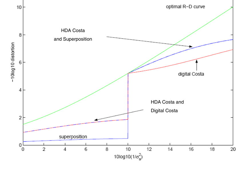
The distortion in the source is shown in Fig.5 for a designed SNR of 10 dB as the actual channel SNR () varies when the source and interference both have unit variance. It can be seen that the distortion in the source is smaller with the HDA Costa scheme than with the digital Costa scheme.
In some case, the distortion in estimating the interference at the receiver may also be of interest and can be obtained by estimating from (38) and (40). The distortion is given below,
| (44) |
It can be seen from Fig. 5 that the distortion in estimating the interference is better for the digital scheme than for the HDA Costa scheme.
In [15], Sutivong et al. have studied a somewhat related problem. They consider the transmission of a digital source in the presence of an interference known at the transmitter with a fixed channel SNR. They study the optimal tradeoff between the achievable rate and the error in estimating the interference at the designed SNR. The main result is that we can get a better estimate of the interference if we transmit the digital source at a rate lesser than the channel capacity. There are important differences our work and that in [15]. First of all, we consider transmission of an analog source instead of a digital source. Secondly, we consider mismatch in the channel, i.e., our schemes are designed to be optimal at the designed SNR and as we move away from the designed SNR, we study the tradeoff between the error in estimating the interference and the distortion in the reconstruction of the analog source. This tradeoff is discussed below.
V-B Generalized HDA Costa Coding under channel mismatch
Next we analyze the performance of the generalized HDA Costa coding under channel mismatch. This case leads to some interesting analysis. By changing the source coding rate of the digital part , we can tradeoff the distortion between the source and the interference in the presence of mismatch.
The different random variables and their relations are given below.
| (45) |
| (46) |
| (47) |
In the above equation (Again, we have dropped the in the expression for .) From the above equations an estimate of as well as is obtained by taking a linear MMSE estimate as all the random variables are Gaussian. The resulting expressions of estimation error and are given by
| (48) |
| (49) |
The performance of the generalized HDA Costa scheme and HDA Costa scheme in relation to digital scheme is shown in fig. 5. For example in separation using digital Costa there is no improvement in our estimate of the analog source, but we get a better estimate of the interference as shown in fig.5. On the contrary for the HDA Costa scheme there is only a small improvement in the estimate of the interference but a good improvement in the estimate of the analog source. The generalized HDA also shows a difference in the estimate for the source and the interference for different rates and performs as a digital Costa for the choice of and as HDA Costa for the choice of . In effect we can tradeoff the estimation error in interference with the source by choosing different values of when there is a channel mismatch.
V-C Hybrid Digital Analog Wyner Ziv
In this case the distortion could be obtained by setting in (42). The actual distortion is given by
| (50) |
This is clearly better than which is what is achievable with a separation based approach. However, we don’t know if this is the optimal distortion that is achievable in the presence of channel mismatch. A simple lower bound on the achievable distortion in the presence of mismatch is to assume that the transmitter knows the channel SNR. Based on this we can analyze the gap in dB between the distorion of HDA Wyner Ziv scheme and the lower bound as follows.
The lower bound on is given by
| (51) |
Now the gap between the analog Wyner-Ziv and the bound at high SNR can be easily calculated as . The gap in db, is hence given by
| (52) |
For example, if our designed SNR is say 10 db, for high SNRs, we loose at most db which is fairly close to the outer bound as shown in Fig. 6.
VI Distortion exponent for HDA Costa and Wyner-Ziv schemes
In this section, we consider the performance of the HDA joint source-channel coding schemes for transmitting a Gaussian source through a Gaussian channel when the actual channel noise variance is not known, but it is known that the variance is always smaller than . Since we are interested in the performance of a single encoding scheme over a wide range of noise variances, a useful measure of performance is the rate of decay of the distortion as a function of the actual noise variance in the limit . More precisely, we define a distortion exponent as
where is the distortion when the noise variance is . Notice that this exponent is quite different from the distortion signal-to-noise ratio (SNR) exponent considered in [18], [19] for the case of slow fading channels. In [18] and [19], the rate of decay of distortion with average SNR is studied by allowing for a family of coding schemes, one for each average SNR. In contrast, we fix the encoding scheme here and consider the rate of decay with the actual channel SNR (i.e., there is no fading).
An upper bound on the achievable can be obtained by assuming that a genie informs the transmitter of and the transmitter chooses an optimal encoding scheme for a noise variance of . Let us assume a general case where there is an interference () which is known at the transmitter and some side information which is related to according to , where is known at the receiver. Then, the distortion for the genie-aided scheme is since an optimal Wyner-Ziv encoder followed by an optimal Costa encoder can be chosen. In this case, the distortion exponent is 1. Notice that in the absence of any side information the distortion for the genie-aided scheme is which also results in an exponent of 1. In the absence of any interference also, the achievable distortion is and the exponent is 1. Thus, for any single encoding scheme, both in the presence and absence of interference and/or side information.
We will now consider the performance of the HDA schemes considered in Section IV. If a joint source channel coding scheme is designed to be optimal when the noise variance is , then the distortion when the noise variance is is given by (from (42) in Section V)
| (53) |
We now consider two cases.
VI-A Absence of Interference
When there is no interference at the transmitter, and, hence, from (53), we can see that the optimal distortion can be obtained for a noise variance of and the optimal distortion exponent of can be obtained. Thus, this scheme performs as well as the genie-aided receiver in the distortion exponent sense.
VI-B Presence of Interference
In the presence of an interference, , and from (53), can be seen to be zero. That is, some amount of residual interference is always present and, hence, in the high SNR limit , the performance is dominated by this residual interference. However, if optimal performance is not desired when the noise variance is , then the optimal exponent of can be obtained using a minor modification to the scheme discussed in Section IV. In the modified scheme, the auxiliary random variable is generated as follows
| (54) |
Note that is chosen to be 1, which is clearly not optimal for a noise variance of . The side information is
| (55) |
and the received signal is
| (56) |
Using arguments similar to those in Section IV, is chosen so as to satisfy . The required condition on can be obtained as follows
| (57) |
Note that and , where . For this choice of , and, hence, . Hence, we get the relation,
Hence, can be chosen to be arbitrarily close to . Now is transmitted and is received. The optimal distortion is obtained as an MMSE estimate of from . The final distortion is given by
| (58) |
It can be seen that as , and, hence, .
VII Applications to Transmitting a Gaussian source with Bandwidth Compression
We now consider the problem of transmitting samples of the i.i.d Gaussian source to a single user in () uses of an AWGN channel with noise variance where the transmit power is constrained to 1. There is no interference in the channel, but since , we will see that the techniques described in the previous sections are useful for this problem.
There at least three ways to achieve the optimal distortion in this case. One is to use a conventional separation based approach. The second one is to use superposition coding and the third one is to use Costa coding. Although, they are all optimal for the single user case, they perform differently when there is a mismatch in the channel SNR and, hence, the last two approaches are briefly described here.
VII-0a Superposition Coding
Here we split the source in two parts and take samples of the source , namely and scale it by creating the systematic signal . We take the other source samples and use a conventional source encoder followed by a capacity achieving channel code resulting in the dimensional vector , where denotes a channel encoding operation and denotes a source encoding operation. Then is normalized so that the average power is . The overall transmitted signal is and the received signal is . At the receiver, the digital part is first decoded assuming the systematic (analog) part is noise and then is subtracted from . Then an MMSE estimate of is formed. For the optimal choice of , the optimal overall distortion can be obtained given by
| (59) |
which is the optimal distortion.
VII-0b Digital Costa Coding

We split the source exactly as in the previous case and one stream is formed as . However, here the digital part assumes that is interference and uses Costa coding to produce with power as shown in Fig. 7. In Costa coding, we define an auxiliary random variable where is the optimum scaling coefficient. At the receiver, the digital part is decoded which means that can be obtained. In spite of knowing exactly, the optimal estimate of is obtained by simply treating as noise since for the optimal choice of , and are uncorrelated. Therefore, an MMSE estimate of is formed assuming were noise. Hence, the overall distortion becomes
| (60) |
Again, minimizing w.r.t. gives
| (61) |
which is the best possible distortion.
VII-0c Hybrid Digital Analog Costa Coding
For the case of , the digital Costa coding part can be replaced by a hybrid digital analog (HDA) Costa coding. We refer to such a scheme as HDA Costa coding. The same power allocation however, remains the same and hence, we can simply use without the need to differentiate the digital and HDA Costa coding. It is quite straightforward to show that for . Hence, the Costa coding approach allocates higher power to the systematic part than the superposition approach, since the systematic part is treated as interference.
VII-A Performance in the presence of SNR mismatch
Now, we consider the same set up as above, but when the actual channel noise variance is , whereas the designed noise variance is .
Case 1:
The distortion for the superposition code can be computed to be the sum of the distortions in the systematic part and the digital part. When , the digital part cannot be decoded and, hence, we assume that the distortion in the digital part is the variance of the source, 1.
| (62) |
Both the digital and HDA Costa coding schemes perform identically when and the distortion for the Costa code can be computed to be
| (63) |
Case 2: In this case, the digital part can be decoded exactly and, hence, the distortion for superposition coding is
| (64) |
For digital Costa coding, the decoder first decodes the digital part when the auxiliary random variable is perfectly known. In the case when , the receiver must form the MMSE estimate of from the channel observation and . Therefore, the overall distortion is
| (65) |
For the HDA Costa coding, we can decode and form MMSE estimates of and separately and, hence, the overall distortion is given by
| (66) |
The performance of the superposition scheme, digital Costa and HDA Costa scheme are shown for an example with in Fig. 8. The designed SNR is defined as whereas the actual SNR is defined as . In the example, the designed SNR is fixed at 10dB and the actual SNR is varied from 0 dB to 20 dB. It can be seen that the Costa coding approach is better than superposition coding when and worse for the other case. The HDA Costa coding scheme performs the best over the entire range of SNRs.
VIII Applications to Broadcasting with Bandwidth Compression
We now consider the problem of transmitting samples of a unit variance Gaussian source in uses of the channel to two users through AWGN channels with noise variances (weak user) and (strong user) with . The channel has the power constraint . We are interested in joint source channel coding schemes that provide a good region of pairs of distortion that are simultaneously achievable at the two users. This problem was considered in [2, 6, 9]. The best known region to date is given by the schemes therein.
Notice that when we design a source channel coding scheme to be optimal for the weak user, the strong user operates under the situation of SNR mismatch explained in Section VII-A with . Similarly, when the system is designed to be optimal for the strong user, for the weak user . Motivated by the fact that for , the HDA Costa coding scheme performs the best, we propose a scheme which is shown in Fig. 9.
There are three layers in the proposed coding scheme. The first layer is the systematic part where out of the samples of the source are scaled by . Let us call this as . The other samples of the Gaussian source are hybrid digital analog Costa coding, treating as the interference and transmits the signal with power in the second layer. So , where and are the optimal scaling coefficient to be used in the hybrid digital analog Costa coding process and is the auxiliary variable. This layer is meant to be decoded by the weak user and, hence, the scaling factor is set to be . That is, this layer sees the third layer also as independent noise.

The third layer is first Wyner Ziv coded at a rate assuming the estimate of at the receiver as side information. The Wyner-Ziv index is then encoded using digital Costa coding assuming and are interference and uses power . Therefore, . This layer is meant for the strong user and, hence, the scaling factor . We then transmit .
At the receiver, from the second layer an estimate of is obtained. This estimate acts as side information that can be used in refining the estimate of for the strong user using the decoded Wyner-Ziv bits. The Wyner-Ziv bits are decoded from the third layer by Costa decoding procedure.
The users estimate the systematic part and non-systematic part by MMSE estimation from the received , the decoded and . So the overall distortion seen at the weak user is
The distortion for the strong user is given by
| (67) |
The corner points of the distortion region corresponding to being optimal for the strong and weak user respectively, can be obtained by setting and , respectively.
The distortion region for this scheme for the case of dB and dB is shown in Fig. 10. The distortion region for three other schemes are also shown. They are the scheme proposed by Mittal and Phamdo in [2], a different broadcasting scheme which uses digital Costa coding in both the layers proposed in [9] (details can be found there) and the broadcast scheme with one layer of superposition coding and one layer of digital Costa coding considered in [6, 9]. This scheme currently appears to be the best known scheme. Notice that in the third layer, instead of using a separate Wynzer-Ziv encoder followed by a Costa code, we could have used the HDA scheme discussed in Section IV with identical results.
The proposed broadcast scheme in Fig. 9 significantly outperforms the scheme in Mittal and Phamdo and the digital Costa based broadcast scheme for this example. The corner points of this scheme also coincide with those of the best known schemes reported in [6, 20].
IX Conclusion and future work
We discussed hybrid digital analog version of Costa coding and Wyner-Ziv coding for transmitting an analog Gaussian source through an AWGN channel in the presence of an interferer known only to the transmitter and side information available only to the receiver respectively. These schemes are closely related to the schemes by Reznic and Zamir [3] and [8], but make the auxiliary random variable model more explicit. We also showed that there are infinitely many schemes that are optimal for this problem, extending the work of Bross, Lapidoth and Tinguely [7] to the side information case. The HDA coding schemes have advantages over strictly digital schemes when there is a mismatch in the channel SNR. This makes them also useful for broadcasting a Gaussian source to two users with different SNRs.
References
- [2] U. Mittal and N. Phamdo, “Hybrid digital-analog HDA joint source-channel codes for broadcasting and robust communications,” IEEE Tran. Info. Theory, vol. 48,no. 5, pp. 1082–1102, May 2002.
- [3] Z. Reznic, M. Feder, and R. Zamir, “Distortion bounds for broadcasting with bandwidth expansion”, IEEE Tran. Info. Theory, vol. 52,no. 8, pp. 3778- 3788, August 2006.
- [4] T. J. Goblick Jr., “Theoretical limitations on the transmission of data from analog sources”,IEEE Tran. Info. Theory, vol. 11,no. 10, pp. 558-567, Oct 1965.
- [5] M. Gastpar, B. Rimoldi and M. Vetterli, “To code, or not to code: lossy source-channel communication revisited”,IEEE Tran. Info. Theory, vol. 49,no. 5 pp. 1147-1158, May 2003.
- [6] V. M. Prabhakaran, R. Puri, and K. Ramachandran, “Hybrid Analog-Digital Strategies for Source-Channel Broadcast” 43rd Allerton Conference on Communication, Control and Computing, Allerton, IL, September 2005.
- [7] S. Bross ,A. Lapidoth, and S. Tinguely, “Superimposed Coded and Uncoded Transmissions of a Gaussian Source over the Gaussian Channel,”Proceedings of the IEEE International Symposium on Information Theory (ISIT), Seattle, USA, 2006.
- [8] Y. Kochman and R. Zamir, “Analog Matching of Colored Sources to Colored Channels,” ISIT 2006, Seattle, USA, July 2006.
- [9] K. R. Narayanan, M. P. Wilson and G. Caire, “Hybrid Digital and Analog Costa Coding for Broadcasting with Bandwidth Compression,” Wireless Communications Lab Technical report, TR-06-107, Texas A&M University, http://wcl3.tamu.edu/research.html, August 25, 2006
- [10] M. Costa, “Writing on Dirty Paper,” IEEE Tran. Info. Theory, vol. 29, No. 3, pp. 439-441, May 1983.
- [11] S. Shamai, S. Verdu, and R. Zamir, “Systematic lossy source/channel coding,” IEEE Trans. Info. Theory, vol. 44, pp. 564–579, March 1998.
- [12] N. Merhav, and S. Shamai, “On joint source-channel coding for the Wyner-Ziv source and the Gel’fand-Pinsker channel,”IEEE Trans. Info. Theory, vol. 49, pp. 2844–2855, November 2003.
- [13] R. Zamir, S. Shamai, and U. Erez, “Nested linear/lattice codes for structured multiterminal binning,” IEEE Trans. Info. Theory, vol. 48, pp. 1250–1276, June 2002.
- [14] U. Erez, S. Litsyn, and R. Zamir, “Lattices which are good for (almost) everything,” IEEE Trans. Info. Theory, vol. 51, pp. 3401-3416, October 2005.
- [15] A. Sutivong, M. Chiang, T. M. Cover, and Y. Kim, “Channel Capacity and State Estimation for State-Dependent Gaussian Channels,” IEEE Tran. Info. Theory, vol. 51, No. 4, pp. 1486-1495, April 2005.
- [16] T. Cover and J. Thomas, Elements of Information Theory, Wiley, 2006
- [17] A. D. Wyner and J. Ziv, “The rate distortion function for source coding with side information at the decoder,” IEEE Tran. Info. Theory, vol. IT-22, no. 1, pp. 1-10, Jan. 1976.
- [18] J. N. Laneman, E. Martinian, G. W. Wornell, and J. G. Apostolopoulos, “Source channel diversity for parallel channels”, IEEE Transactions on Information Theory, vol. IT-51, no. 10, pp. 3518–3539, Oct 2005.
- [19] T. Holliday and A. J. Goldsmith, “Joint source and channel coding for mimo systems”, Allerton Conf. Commun. Control and Computing, pp. 1302–1311, Monticello IL, USA, Oct. 2004.
- [20] K. R. Narayanan, G. Caire and M. P. Wilson, “Duality Between Broadcasting with Bandwith Expansion and Bandwidth Compression”, Proc. Intl. Symp. Info. Theory, Nice, France 2007.