Composite self-similar solutions for relativistic shocks:
the transition to cold fluid temperatures

The energy and Lorentz factor that we expect in the ejecta in supernovae and gamma-ray bursts are important because they constrain the amount of energy that can be deposited in the photons we observe from these explosions. Previous work on the ejecta, notably [10], uses as a starting point the analytic solutions of [3] for a planar relativistic shock propagating into cold surroundings: by the time the shock reaches the outer envelope of the star, the likely source of the ejecta, it has accelerated to relativistic speeds and its geometry is planar. Several authors have described the reltivistic shock’s propagation and acceleration through this envelope [1, 8, 9, see, for example,], but the work of [3] and other analytic work on the flow from a relativistic shock that breaks out of a star [5, 7] show that significant acceleration also occurs after the fluid is shocked. As the hot fluid expands adiabatically, its thermal energy is converted to bulk kinetic energy.

Since all the above authors assume an ultrarelativistic equation of state for the fluid, the final Lorentz factor their solutions predict for the fluid is formally infinite as the fluid never cools. They avoid this difficulty by following fluid elements in the flow only to the point where the fluid temperature becomes nonrelativistic and approximating the final coasting Lorentz factor as the one given by their solutions at that point. They thus find that the final Lorentz factor of a given fluid element scales as $\gamma_{0}^{1+\sqrt{3}}$ where $\gamma_{0}$ is the Lorentz factor acquired by the fluid when it is shocked. This method cannot accurately account for acceleration that occurs around the time when the fluid cools to nonrelativistic temperatures and can only produce approximate relations for the energy and velocity of the ejecta. While [4] relax the assumption of an ultrarelativistic fluid in their work on this problem, they cannot completely characterize the acceleration while the fluid is cooling either.

We approach this problem by introducing a new kind of self-similar solution for the cooling and expanding fluid. In this solution, we require that the fluid move at relativistic speeds but relax the assumption that the fluid be hot. We place the characteristic position at the point where the fluid temperature is transrelativistic. We thus exploit the self-similarity of the transition between hot and cold fluid in the flow rather than the self-similarity in the acceleration of the hot fluid. Indeed, this flow when taken in its entirety is not self-similar: the size scales that characterize the acceleration and the hot/cold transition evolve with time according to different power laws. In other words, the entire flow is a composite of two distinct self-similar solutions. In §II we summarize the solution for the hot fluid, which gives the initial conditions for this new solution. In §III we derive the new solution, and in §IV we describe the behavior of fluid elements in the composite solution. In §V we explain changes in the flow’s behavior for very shallow initial density profiles in the stellar envelope. In §VI we discuss the behavior of the flow at late times and relate the elements’ final Lorentz factors and the Lorentz factors to which they were initially shocked. In §VII we find regions of the flow where spherical corrections are important, and in §VIII we summarize our findings and discuss them in the context of previous work. We take the speed of light to be $c=1$ throughout our discussion.

We are interested in the behavior at late times of a fluid flow which begins as a relativistic shock propagating through the outer layers of a star with a polytropic envelope. As long as the distance between the front of the flow and the original location of the star’s surface is small compared to the star’s radius, the geometry is planar. So we seek a self-similar solution to the following hydrodynamic equations representing energy, momentum, and mass conservation:

The solution we seek must be connected to the hot flow, whose behavior is well understood: [9] and [5] derive the self-similar solution before the shock breaks out of the star and [7] derives the post-breakout solution. Here we simply state these results. We take $R(t)$ to be the characteristic position in the solution, and we set $R=0$ and $t=0$ at breakout. We take $\Gamma$, $P$, and $N$ to be the characteristic Lorentz factor, pressure, and number density; $R$ and $\Gamma$ are related in that $\dot{R}=\sqrt{1-1/\Gamma^{2}}\simeq 1-1/\left(2\Gamma^{2}\right)$. We define

Here $k$ gives the unshocked density profile in the stellar envelope: assuming gravity is constant in the star’s outermost layers and unshocked pressure and density are related by a power law, the density is given by a power law $\rho\propto|x|^{-k}$ where $x$ is the position relative to the star’s surface. This implies $-3\leq k\leq-3/2$ for degenerate and convective envelopes and $k=-17/13$ for Kramers opacity envelopes. We consider here the regime $k<-\left(1+\sqrt{3}\right)/3$, which includes all of these profiles; we explain this choice of maximum $k$ in §III. We write the solutions in the form

where the similarity variable is

Note that this expression is equivalent to

taken in the limit where $\Gamma\gg 1$, or where $t\simeq R(1+1/\left(2(m+1)\Gamma^{2}\right)$, so that the flow’s characteristic length scale is $t-R=R/\left(2(m+1)\Gamma^{2}\right)$.

Mathematically, the pre- and post-breakout solutions differ only in the ranges in $\chi$ which apply. They are

where

These ranges differ because the sign of $R$ and the interpretation of the characteristic values $\Gamma$, $P$, $N$, and $R$ change at breakout. Before breakout, $R<0$ and $\Gamma$, $P$, $N$, and $R$ are associated with the shock front; after breakout, $R>0$ and $\Gamma$, $P$, $N$, and $R$ are associated with a fluid element which has expanded by a factor of order unity.

The solutions are then completely specified by an expression for $m$ in terms of $k$, which gives the time evolution of the flow, and expressions for $g$, $f$, and $h$ in terms of $\chi$, which give the spatial profiles for the hydrodynamic variables:

Thus defined, Eqs. 5, 6, 7 satisfy the hydrodynamic equations with the equation of state $p=e/3$. They are an accurate description of the flow with $k<-\left(1+\sqrt{3}\right)/3$ only where the fluid is hot, or where $p/n\gg 1$. As the fluid expands and accelerates after breakout, it cools adiabatically from the back of the flow towards the front [7]. As a result, the above post-breakout solution holds only for a region at the front of the flow, and this region shrinks with time. This solution sets the boundary conditions for the new solution we seek: as we approach the vacuum interface at $\chi=0$, where the fluid is still hot, the new and the old solutions must coincide.

We are interested in the behavior at late times of a fluid flow that begins as a relativistic shock propagating through the outer layers of a star with a polytropic envelope. We understand the behavior of the part of the flow that is hot ($p/n\gg 1$) and therefore obeys the equation of state $p=e/3$: it follows the self-similar solution given in Eqs. 4, 10–16. We note for convenience in our discussion below that the self-similar variable $\chi$, as given by Eq. 9, is equivalent to

taken in the limit where $\Gamma\gg 1$, or where $t\simeq R(1+1/(2(m+1)\Gamma^{2})$. The implied characteristic length scale is $t-R=R/(2(m+1)\Gamma^{2})$.

As the fluid expands and accelerates after breakout, it cools adiabatically from the back of the flow towards the front. At late times, then, the post-breakout solution of §2, which we will refer to here as the “hot solution,” holds only for a region at the very front of the flow, and this region shrinks with time. The hot solution sets the boundary conditions for the new solution we seek: as we approach the vacuum interface at $\chi=0$, the two solutions must coincide.

In the new solution, which we will refer to as the “cooling solution,” we must include cold fluid. We therefore use the equation of state

rather than the ultrarelativistic $p=e/3$. Although this equation of state applies only to fluids with adiabatic index 4/3, our analysis can be easily modified to accommodate an arbitrary equation of state of the form

where $F$ is an invertible function since the hydrodynamic equations can be written in self-similar form with any such equation of state.

We must also specify a characteristic scale and define the characteristic Lorentz factor, pressure, and number density to be consistent with this scale. We seek the profiles of the hydrodynamic variables in the region where the fluid temperature transitions from hot to cold; the natural scale for this transition is the distance $\delta$ between the vacuum interface, where the fluid is hottest, and the point where the fluid temperature becomes nonrelativistic. We set this point to be where $p/n=1$. Then the similarity variable is

and, by analogy with the hot solution, we express $\gamma$, $p$, and $n$ as

We choose $\bar{\Gamma}$, $\bar{P}$, and $\bar{N}$, the new characteristic values of the Lorentz factor, pressure, and number density, to match the $\gamma$, $p$, and $n$ values given by the hot solution where $p/n=1$. We take $\chi_{\mathrm{cold}}$ to be the value of the old similarity variable $\chi$ corresponding to $p/n=1$ in the hot solution:

This choice of characteristic values dictates

In the limit of late times, when $\delta\ll R/\Gamma^{2}$ and $g\chi-\left(g\chi\right)_{0}\ll\left(g\chi\right)_{0}$, Eqs. 24 and 17 give

Note that the characteristic scale $t-R\sim R/\Gamma^{2}$ in the post-breakout solution for the hot fluid is different from the new scale $\delta$. $R$ is the location of a fluid element that has expanded by a factor of order unity since breakout. Because $R$ evolves according to the finite characteristic Lorentz factor $\Gamma$, $R$ lags farther and farther behind the front of the flow, where the Lorentz factors are arbitrarily large. Since $\Gamma$ decreases with time as per Eq. 4, $t-R$ increases with time. In the limit of late times, then, $R$ lags far behind the portion of the flow where the fluid remains hot and $t-R$ becomes much larger than the space occupied by the hot fluid. In other words, the scale $t-R$ that characterizes the hot solution becomes irrelevant to the transition between hot and cold fluid that is of interest here.

To get $\bar{\Gamma}$ and $\delta$ as functions of time, we apply Eqs. 14–16 at the point $p/n=1$. We use $P/N=\Gamma/(3\sqrt{2})$, a relation that follows from the shock jump conditions applied in the pre-breakout solution.

This gives

at late times, when $g(\chi_{\mathrm{cold}})\cdot\chi_{\mathrm{cold}}\simeq\left(g\chi\right)_{0}$. Solving Eq. 30 for $f(\chi_{\mathrm{cold}})$ or $h(\chi_{\mathrm{cold}})/\sqrt{g(\chi_{\mathrm{cold}})}$ similarly gives

Note that $k=-\left(1+\sqrt{3}\right)/3\simeq-0.91$ makes $a$ and $b$ diverge in Eqs. 34 and 36. This $k$ marks a qualitative change in the behavior of the flow which we discuss further in § V.

We now proceed to solve the hydrodynamic equations for the relevant range in $k$. We use the equation of state Eq. 18 to rewrite Eq. 1, Eq. 3, and the difference equation obtained by subtracting Eq. 2 from Eq. 1. We take the limit $\gamma\gg 1$. We rewrite the differentiation operators as

and substitute these and Eqs. 24-27, 34, and 36 to get

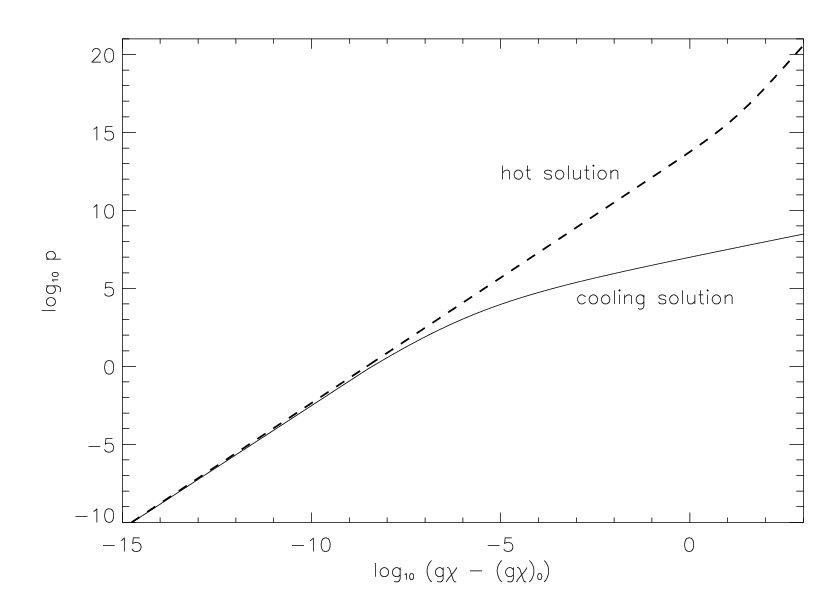
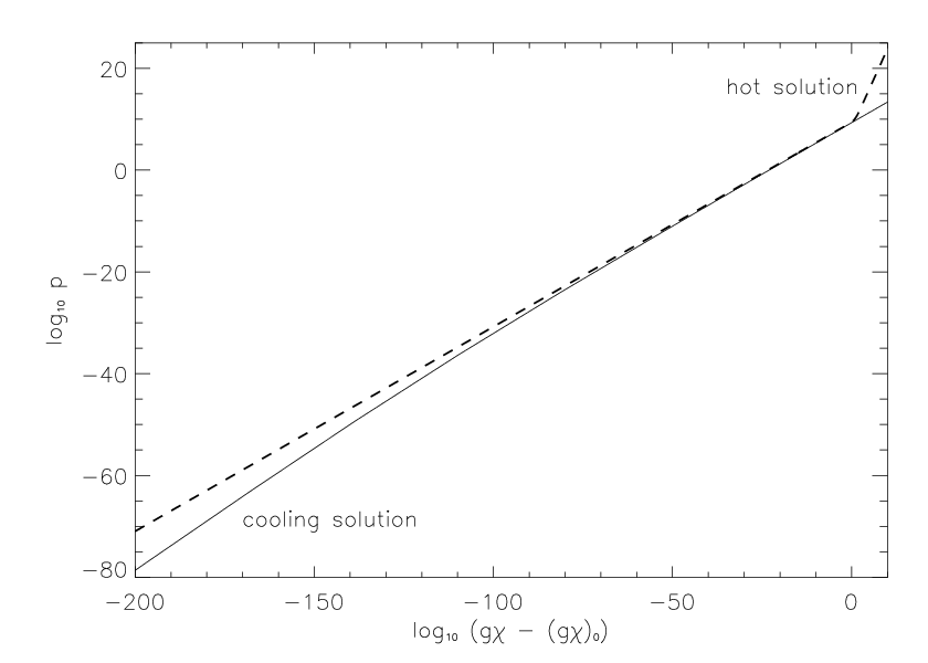
We substitute Eqs. 29 and 35 into Eqs. 39, 40, and 41 and integrate this ODE system numerically to produce the solution shown in Figures 1, 2, and 3. These figures also compare our solution to a one-dimensional numerical simulation of a relativistic planar shock wave which accelerates through and breaks out of a $k=-3$ medium and then expands and cools through the transrelativistic regime. The initial conditions used in the simulation represent the shock as an unresolved contact discontinuity with $\Gamma=5$ at $x=-10^{-5}$ at starting time $t=-1.0\times 10^{-5}$. The simulation grid contains 400 fluid elements spread logarithmically over two orders of magnitude in $x$; our calculation follows these elements until time $t=2.6\times 10^{8}$.

We can check that the behavior of this solution at large $\xi$—where the fluid is very cold and where the hot solution and cooling solution differ most—is physical. Consider a fluid element many distance scales $\delta$ behind the vacuum interface at position $t-x\gg\delta$. This fluid element must have become cold at some time $t_{\mathrm{cold}}\ll t$; as a result, it has long since stopped accelerating and has spent most of the time interval $t-t_{\mathrm{cold}}$ coasting at its current Lorentz factor $\gamma$. Then this fluid element has

so at large $\xi$ we expect

We cannot get exact relations for $\bar{f}$ and $\bar{h}$ in the large $\xi$ limit in this way because $p$ and $n$ change significantly while the fluid element finishes its acceleration. However, we can check the scalings of $\bar{f}$ and $\bar{h}$ with $\xi$. Because the fluid elements far behind the front are coasting with Lorentz factors that are virtually constant in time, the volume of each fluid element increases linearly with time. This implies

for a single fluid element. From the definitions of $\bar{\Gamma}$, $\bar{P}$, and $\bar{N}$ in Eqs. 24, 25, and 26, we know $\gamma(\xi=1)/\bar{\Gamma}$, $p(\xi=1)/\bar{P}$, and $n(\xi=1)/\bar{N}$ are constant in time. Then for a single fluid element,

Since

we have

A similar calculation yields

That the relations in Eqs. 43, 47, and 48 hold at large $\xi$ is shown in Figure 4.

As discussed in § II and III, the hot fluid close to the vacuum interface and the cooling fluid further back in the flow obey two different self-similar solutions in which both the time evolution and the physical interpretation of the characteristic length scale, Lorentz factor, pressure, and density differ. In other words, we describe the entire post-breakout flow—which, when taken as a whole, is not self-similar—by a composite of two self-similar solutions built up around the two different length scales which characterize different portions of the flow. This to our knowledge is the first such ‘composite solution’ found. [2], for example, also uses two self-similar solutions in a description of a single flow—specifically, the interaction between an expanding shell of fluid and a stationary external medium. However, his solutions have the same characteristic length scale and time evolution; they differ only in the shapes of their profiles and in the disjoint regions of the flow in which they operate. They may be considered as a single self-similar solution in which the pressure, velocity, and density profiles are piecewise functions of position.

We can check that the behaviors of fluid elements and sound waves in the hot solution and the cooling solution are consistent. The characteristic position $R$ in the hot solution moves backwards relative to the vacuum interface with time because $\Gamma$ decreases with time. By contrast, the characteristic position $t-\delta$ in the cooling solution moves forwards relative to $ct$ because fluid elements at the back of the solution cool faster than those at the front, and $t-\delta$ marks the location of a fluid element that has just cooled. We confirm the forward motion by looking at Eq. 35, which indeed gives $t\dot{\delta}/\delta<0$ for the range of $k$ of interest ($k<-\left(1+\sqrt{3}\right)/3$). We expect fluid elements in the cooling solution to move backwards in the solution, or towards larger $\xi$: every fluid element must eventually finish accelerating and become cold, so the point $t-\delta$ that marks the hot/cold transition must overtake every fluid element. Indeed, the time derivative of $\xi$ following a fluid element,

is always positive since $t\dot{\delta}/\delta<0$. Fluid elements in the hot solution move forwards with time, towards smaller $g\chi$, since they accelerate while $R$ decelerates. The advective time derivative of $\chi$,

is always negative since $g\chi\geq\left(g\chi\right)_{0}>4+2\sqrt{3}$ everywhere.

If the proper sound speed in the fluid is $\beta_{s}=\sqrt{4/3}\bar{f}^{1/2}\bar{g}^{1/4}\bar{h}^{-1/2}$, then the motion of a sound wave in the cooling solution is given by

where the signs denote forward- and backward-propagating sound waves. Again, $t\dot{\delta}/\delta<0$, so $d\xi_{\pm}/dt>0$ everywhere and all sound waves move backwards in the cooling solution. In other words, all fluid elements are disconnected from the vacuum interface. In the sense that the front is disconnected from the fluid far back in the flow, the cooling solution is similar to Type II solutions. However, in contrast to the usual Type II scenario, there is no sonic point constraining the solution.

There is a caveat in this composite view of the flow for the density profiles $k<-\left(1+\sqrt{3}\right)/3$ discussed in the preceding sections. At early times when $\Gamma\gg 1$, all the fluid elements which have accelerated by at least a factor of order unity are those with $p/n\gtrsim\Gamma$; slower and cooler fluid elements still have very nearly the same temperatures and speeds as they had just after being shocked. So the only fluid elements with $p/n$ of order unity or smaller are those which were never shocked to relativistic temperatures, and the part of the flow moving relativistically can be described with the hot solution alone. At late times when the cold solution is relevant, the hot solution applies only in a region at the front of the flow whose size is much smaller than the characteristic scale $R/\Gamma^{2}$. In this small region, the profiles of the hydrodynamic variables in hot solution appear very nearly scale free, and the cooling solution approaches the resulting power-law profiles toward the front of the flow, in the limit of small $\xi$. Then the hot solution is unnecessary to the description of the flow at these late times, so we can think of the flow as following the hot solution at early times and transitioning to the cooling solution when $\Gamma=1$. Figure 5 is a schematic of the composite flow at these late times.

However, a composite of the hot and cooling solutions is essential in describing the flow for density profiles $-\left(1+\sqrt{3}\right)/3\leq k<0$, which we discuss in the next section.

We restricted our discussion of the hot and cooling solutions in § II, III, IV to initial density profiles $k<-\left(1+\sqrt{3}\right)/3$. That the initial density decrease toward the star’s surface requires $k<0$, but so far we have neglected the interval $-\left(1+\sqrt{3}\right)/3\leq k<0$. To describe the flow for these $k$, we return to the singularity at $k=-\left(1+\sqrt{3}\right)/3$ noted in § III and examine the behavior of $\left(g\chi\right)_{\mathrm{cold}}=g(\chi_{\mathrm{cold}})\cdot\chi_{\mathrm{cold}}$.

Eq. 30 implies

For $-\left(1+\sqrt{3}\right)/3<k<0$, integration of Eq. 52 shows that $\left(g\chi\right)_{\mathrm{cold}}$ is a double-valued function of time until the entire flow cools. As $t\rightarrow 0$ from above, $\left(g\chi\right)_{\mathrm{cold}}\rightarrow\{\left(g\chi\right)_{0},\infty\}$; for positive times, the smaller value of $\left(g\chi\right)_{\mathrm{cold}}$ increases and the larger value decreases with time until $\left(g\chi\right)_{\mathrm{cold}}$ becomes single-valued at $\left(g\chi\right)_{\mathrm{cold}}=2\left(3+4/\sqrt{3}\right)$, which occurs at a finite time. In other words, fluid cools quickly both at the front, where the expansion timescale is shortest, and at the very back, where the shocked fluid is coldest.

Since $\left(g\chi\right)_{\mathrm{cold}}$ becomes single-valued at a $\left(g\chi\right)_{\mathrm{cold}}$ of order unity, the value of $g$ corresponding to the larger value of $\left(g\chi\right)_{\mathrm{cold}}$ is always of order unity or smaller. But $g=1$ for a fluid element which has accelerated by a factor of order unity, so this larger $\left(g\chi\right)_{\mathrm{cold}}$ tracks fluid elements which cool before or just as they manage to accelerate by a factor of order unity. These fluid elements cannot have been shocked to relativistic temperatures, so we focus on the evolution of the smaller value of $\left(g\chi\right)_{\mathrm{cold}}$ as it moves through the front of the solution. In contrast to the $k<-\left(1+\sqrt{3}\right)/3$ case, the fluid near the front cools from the vacuum interface backwards, from the fastest-moving toward slower-moving fluid, and the fluid farthest forward is coldest: $\bar{\Gamma}$ decreases with time and $\bar{P}$, $\bar{N}$, $\delta$ increase with time. Fluid elements just behind the front—specifically, those with $g\chi-\left(g\chi\right)_{0}\ll 2+2/\sqrt{3}+2k\sqrt{3}$ —always have $\left(g\chi\right)_{\mathrm{cold}}\simeq\left(g\chi\right)_{0}$, so they obey Eqs. 34-36. Then the discussion of the cooling solution in § III applies in the limit of small positive times, when the front of the flow is cooling, except in that the initial conditions used to integrate Eqs. 39-41 are set by matching to the hot solution far back in the cooling flow, at $\xi\gg 1$, rather than at the vacuum interface. Between breakout and the time when all the fluid cools, the flow contains both hot and cold fluid moving at relativistic bulk speeds; it therefore follows a true composite of the hot and cooling solutions. Figure 6 shows a schematic of this composite solution.

As in the $k<-\left(1+\sqrt{3}\right)/3$ case, fluid elements move forwards in the hot solution with time according to Eq. 50. No qualitative change in the time evolution of the scale $R$ —or, therefore, in the behavior of fluid in the hot solution—occurs as $k$ increases through $-\left(1+\sqrt{3}\right)/3$. In contrast to the $k<-\left(1+\sqrt{3}\right)/3$ case, fluid elements move forwards in the cooling solution as well. Eq. 42, which still holds in the limit $t-x\ll\delta$, implies $\bar{g}\xi\geq 2-\sqrt{3}$, while Eq. 35 implies $t\dot{\delta}/\delta>1$. Then from Eq. 49 we have $D\xi/Dt<0$.

For $k=-\left(1+\sqrt{3}\right)/3$, $\left(g\chi\right)_{0}=3\left(2+4/\sqrt{3}\right)$, so $\left(g\chi\right)_{\mathrm{cold}}$ is single-valued and $\left(g\chi\right)_{\mathrm{cold}}-2\propto t^{-1}$. Then there is a finite time at which $\left(g\chi\right)_{\mathrm{cold}}$ reaches $\left(g\chi\right)_{0}$, $\delta$ shrinks to 0, and the entire flow cools. Also, at any $t>0$, Eq. 15, 16 imply that the temperature at the front of the flow, where $g\chi-\left(g\chi\right)_{0}\ll\left(g\chi\right)_{0}$, is roughly independent of position, and the temperature at the vacuum interface is finite; all the fluid at the front cools at the same rate. Though Eq. 35 does not work for this $k$, we know $\delta$ decreases monotonically to 0 with time, so Eq. 49 gives $D\xi/Dt>0$. So fluid elements move backwards in the cooling solution until $\left(g\chi\right)_{\mathrm{cold}}=\left(g\chi\right)_{0}$ and $\delta=0$.

Earlier analytic work has established that the final Lorentz factor $\gamma_{\mathrm{final}}$ of a given fluid element should scale according to

where $\gamma_{\mathrm{shocked}}$ is the fluid element’s Lorentz factor immediately after it is shocked in the pre-breakout flow and the coefficient $K$ is independent of $\gamma_{\mathrm{shocked}}$ [3, 7]. [10] have found numerically that $K\simeq 2.6$ for $k=-3$. They note, and we confirm from our own experience, that it is difficult to continue numerical simulations until the very end of the fluid acceleration since the conversion of thermal to bulk kinetic energy is quite slow: Figure 4 indicates significant acceleration until $\xi\sim 10^{10}$. To estimate the coefficient, [10] applied correction factors to their simulation results of up to $\sim$50% for fluid elements with final Lorentz factors of order $\sim 10^{3}$.

We can find $\gamma_{\mathrm{final}}$ for a given fluid element directly from our pre- and post-breakout solutions. To track the acceleration of the fluid element while it is hot, we take the advective time derivative of $\gamma$ in the pre- and post-breakout solutions for the hot fluid and integrate with the proper limits.

Before breakout, the fluid element’s $g\chi$ goes from $g\chi=1$ when it is shocked to $g\chi\rightarrow-\infty$ at breakout. After breakout, the fluid element’s $g\chi$ goes from $g\chi\rightarrow\infty$ to $g\chi\simeq\left(g\chi\right)_{\mathrm{cold}}$. So when the fluid becomes cold, we have

To find the correct $g\chi$ at which to evaluate the above, we set $C=\gamma f/h$ to be the temperature (up to a factor of 3) at the $g\chi$ of interest and use Eqs. 15, 16 to express $(g\chi-2)/(g\chi-\left(g\chi\right)_{0})$ in terms of $C$. This gives

To this we add the extra factor given by the cooling solution to get the coefficients $K$ shown in Figure 7. In particular,

This result is close to the results of [10], who find a coefficient of $\sim 2.6$ when $k=-3$. Note that $p/n=1$ corresponds to $C^{-\sqrt{3}}=0.149$: $\gamma$ grows by a factor of $\sim 15$ after the fluid element becomes nominally cold.

The growth of $\gamma$ as a function of the temperature for a single fluid element is shown in Figure 8, which also shows good agreement between the cooling solution and direct numerical simulations of the hydrodynamic equations. Because the Lorentz factors near the front of the flow in particular become very large at late times, it is difficult to produce numerical simulations that remain accurate as the fluid cools all the way to $p/n\ll 1$. As a result, the numerical simulation shown in Figure 8 cuts off while the fluid Lorentz factor is 9% smaller than the final Lorentz factor predicted by the cooling solution.

We can estimate the ranges of initial positions and Lorentz factors for which corrections to our planar solutions due to the star’s spherical geometry are important. Spherical geometry significantly affects a given fluid element’s acceleration if the distance between the fluid element and the star’s center doubles before the fluid element finishes accelerating. Once the fluid element has traveled a distance comparable to $R_{*}$, the star’s radius, it has expanded significantly in directions perpendicular to its motion; planar solutions cannot account for this transverse expansion. For our estimate we therefore check which fluid elements have cooled to $p/n\sim 1$ by time $t\sim R_{*}$.

Consider a fluid element whose position before being shocked is $x_{\mathrm{init}}<0$. According to the relativistic shock jump conditions, immediately after this fluid element is shocked it has

where $\Gamma$ is the shock Lorentz factor in the pre-breakout solution and $x_{\mathrm{rel}}$ is the position of the shock when it first becomes relativistic, or when $\Gamma\simeq\sqrt{2}$. Right after breakout our fluid element follows the hot solution; when it reaches $\chi=1$, it has accelerated and expanded by a factor of order unity since being shocked, so it still has $p/n\sim(x_{\mathrm{init}}/x_{\mathrm{rel}})^{-m/2}$. Also, at this point $\Gamma\sim\gamma_{\mathrm{init}}$ so the time is$\sim|x_{\mathrm{init}}|$. We track the temperature of the fluid element over time until it reaches $p/n=1$ by taking the advective time derivative of $p/n$:

where the final equality holds while the fluid element is at $g\chi-\left(g\chi\right)_{0}\ll\left(g\chi\right)_{0}$ —that is, near the front of the flow, where most of the acceleration takes place. We then have

We now impose the condition $p/n\sim 1$ at or before $t\sim R_{*}$ to get the scaling

Sphericity corrections are unimportant for fluid elements which satisfy this condition. For $0>k\geq-\left(1+\sqrt{3}\right)/3$, the exponent on the right hand side is not positive, so spherical corrections are unimportant as long as $|x_{\mathrm{rel}}|<R_{*}$. On the other hand, for $k<-\left(1+\sqrt{3}\right)/3$ spherical corrections are important for a layer of fluid initially adjacent to the star’s surface: in our self-similar solutions for these $k$ values, fluid elements that start arbitrarily close to the star’s surface will take arbitrarily long to cool.

The equivalent condition on $\gamma_{\mathrm{init}}$, the Lorentz factor of a given fluid element just after being shocked, is

the one for $\gamma_{\mathrm{final}}$, the fluid element’s Lorentz factor after it finishes accelerating, is

We have derived a new self-similar solution, the cooling solution, for the flow that results when a relativistic shock breaks out of a polytropic envelope. The cooling solution is based on our identification of the characteristic position with the point where the fluid cools to nonrelativistic temperatures. The cooling solution shows that the transition between hot and cold fluid in the flow is self-similar even though this transition is not included—indeed, is not self-similar—in the old post-breakout solution for the hot fluid alone. We present a description of a non-self-similar flow using a composite of two distinct self-similar solutions in which the time evolution and physical interpretation of the characteristic scales differ. As the envelope’s original density profile $k$ increases past $k=-\left(1+\sqrt{3}\right)/3$, the flow dictated by the composite solution changes qualitatively from one where the slowest fluid at the back of the flow cools most quickly to one where the fastest fluid at the front of the flow cools most quickly.

The cooling solution allows accurate calculation of the final Lorentz factors of the shocked fluid elements. Given a stellar model for a core-collapse supernova progenitor and an input explosion energy, we can extract the initial density profile of the progenitor envelope and the initial shock velocity and use the cooling solution to find the Lorentz factor and kinetic energy profiles in the relativistic ejecta after the ejecta finish accelerating. This provides an accurate value for the energy available to produce observable lightcurves via interaction between the ejecta from the model explosion and the progenitor’s surroundings.

[4] also investigate cooling in the flow produced after a relativistic shock breakout. They focus on a $k=-3$ density profile and use as starting point the work of [5], who found a numerical self-similar solution for the hot planar flow in a Lagrangian framework. While [4] also describe the cooling flow with a system of ODEs, they conclude that no self-similar solution exists for the cooling flow: instead of adopting a new characteristic scale in writing the ODEs for the cooling flow, they retain the characteristic scale relevant to the hot solution. Because they do not recognize the self-similarity of the flow, and because they do not integrate until the fluid has cooled enough, they find that initially hot fluid does not stop accelerating. As a result they cannot express the final Lorentz factors of given fluid elements in terms of the initial ones.

In addition, [4] focus on corrections to their planar flow due to spherical geometry. They perturb the hydrodynamical equations to lowest order in a new variable equal to the position coordinate scaled to the stellar radius. Their non-self-similar solutions to the perturbed equations agree well with their numerical simulations only at very early times, before the fluid has expanded by a factor of $\sim$2. They look at sphericity effects in the cooling flow using numerical simulations and find that for fluid whose initial fractional distances from the star’s surface to its center lie between about $4\times 10^{-4}$ and $3\times 10^{-3}$, sphericity effects change the final velocities by factors of order unity in simulations with $k=-3$, $\Gamma=10^{5}$ and $10^{6}$ at $t=1$, and $R_{*}=3.3$ in units where $c=1$. Although such a fast shock is unrealistic since it would have $\Gamma\sim 10^{4}$ or $10^{5}$ at the star’s center, our scaling in §VII also indicates that sphericity corrections would be important for these parameters.

[10] also consider sphericity corrections for the density profile $k=-3$, but they treat the opposite limit of mildly relativistic shocks with $\Gamma-1$ ranging from about $7\times 10^{-3}$ to $0.28$ when the shock is halfway from the star’s center to its surface. Only their two most energetic numerical calculations of sphericity effects attain shock Lorentz factors $\Gamma>\sqrt{2}$, so nonrelativistic estimates of sphericity corrections are relevant for most of the regime they consider. However, those two most energetic shock calculations show that for the relativistic fluid elements shocked to initial Lorentz factors between about $\sqrt{2}$ and $4$, sphericity decreases the final velocities by twenty to thirty percent. Our scaling in §VII indicates that for those two scenarios, sphericity corrections should be important for fluid elements shocked to Lorentz factors larger than about 1.7 and 2.4 respectively; this is roughly consistent with the findings of [10].

References

- [1] Best, P., and R. Sari 2000. Second-type self-similar solutions to the ultrarelativistic strong explosion problem. Physics of Fluids 12, 3029–3035.
- [2] Chevalier, R. A. 1982. Self-similar solutions for the interaction of stellar ejecta with an external medium. ApJ 258, 790–797.
- [3] Johnson, M. H., and C. F. McKee 1971. Relativistic Hydrodynamics in One Dimension. Phys. Rev. D 3, 858–863.
- [4] Kikuchi, R., and T. Shigeyama 2007. Relativistic Flows after Shock Emergence. ApJ 657, 860–869.
- [5] Nakayama, K., and T. Shigeyama 2005. Self-similar evolution of relativistic shock waves emerging from plane-parallel atmospheres. ApJ 627, 310–318.
- [6] Pan, M. 2006. Slices of theoretical astrophysics: solar system dynamics and relativistic explosions. PhD thesis, California Institute of Technology.
- [7] Pan, M., and R. Sari 2006. Self-similar solutions for shocks breaking out of stars with polytropic envelopes. ApJ 643, 416–422.
- [8] Perna, R., and M. Vietri 2002. A self-similar solution for the propagation of a relativistic shock in an exponential atmosphere. ApJ 569, L47–L50.
- [9] Sari, R. 2006. First- and second-type self-similar solutions for implosions and explosions containing ultra-relativistic shocks. Physics of Fluids 18.
- [10] Tan, J. C., C. D. Matzner, and C. F. McKee 2001. Trans-Relativistic Blast Waves in Supernovae as Gamma-Ray Burst Progenitors. ApJ 551, 946–972.