Biological activity in the wake of an island close to a coastal upwelling
Abstract
Hydrodynamic forcing plays an important role in shaping the dynamics of marine organisms, in particular of plankton. In this work we study the planktonic biological activity in the wake of an island which is close to an upwelling region. Our research is based on numerical analysis of a kinematic flow mimicking the hydrodynamics in the wake, coupled to a three component plankton model.
We use parameter values of relevance for the Canary wake, and the main results for a realistic range of parameters in this area area are: a) Primary production is enhanced in the region of the wake opposite to the upwelling zone. b) There is a strong dependence of the productivity on the inflow conditions of biological material entering the wake transported by the main current. Finally c) we show that under certain conditions the interplay between wake structures and biological growth leads to plankton blooms inside mesoscale hydrodynamic vortices that act as incubators of primary production.
Keywords: plankton; island wake; primary production; upwelling; vortex dynamics
1 Introduction
Understanding the influence of hydrodynamic motions on the growth, productivity and distribution of marine organisms, especially in the context of plankton dynamics, is a major challenge recently addressed from a variety of perspectives (Mann & Lazier, 1991; Denman & Gargett, 1995; Abraham, 1998; Peters & Marrasé, 2000; Károlyi et al., 2000; López et al., 2001a; López et al., 2001b; Martin et al., 2002; Martin, 2003). Vertical transport processes of nutrients are recognized as key factors controlling plankton productivity (Denman & Gargett, 1995). In particular, upwelling areas in the world’s oceans are of fundamental importance for the growth of phytoplankton which is the base of oceanic food webs. They are characterized by nutrient rich waters coming to the surface from depths of over meters. Nutrient enrichment enhances phytoplankton growth close to the upwelling regions, giving rise to an increase in zooplankton and fish populations in the area. More recently, the importance of horizontal fluid motion has also been pointed out (Abraham, 1998; López et al., 2001b; Hernández-García et al., 2002; Hernández-García et al., 2003; Martin, 2003). Mesoscale stirring redistributes and mixes plankton and nutrients laterally, giving rise also to enhanced productivity (Martin et al., 2002), or to bloom initiation (Reigada et al., 2003), and affects species competition and coexistence (Károlyi et al., 2000; Bracco et al., 2000). Satellite images illustrate the interaction between horizontal mesoscale motions and plankton dynamics.
Vertical upwelling and strong mesoscale activity occur simultaneously in several places of the globe. A stronger impact and a high complexity of the physical-biological interactions are expected there. Some of these areas are the Benguela zone, the Humboldt Current, or the Canary islands.
Though the phenomena we discuss are rather general, we illustrate them by using the Canary islands, which are close to the northwestern African coast, as a specific example. There, upwelling occurs at the African coast because of Ekman pumping induced by the dominant winds, and in addition, the Canary islands constitute an obstacle for the main ocean current in the area, flowing from Northeast to Southwest, originating a strong mesoscale hydrodynamic activity in their wake. The interaction between the vortices in the wake and the Ekman flow transporting nutrient-rich waters from the coastal upwelling seems to be at the heart of the observed enhancement of biological production in the open Atlantic ocean close to the Canary region. Motivated by this situation, the aim of this paper is to study, in a more general framework, the role of wake vorticity in redistributing upwelled nutrients and influencing phytoplankton growth.
To this end we combine the kinematic model flow introduced in Sandulescu et al. (2006) with a simple model of a Nutrient-Phytoplankton-Zooplankton (NPZ) trophic chain, and study the impact of the flow characteristics on the biological dynamics, particularly on the primary production (). We will use mainly parameter values of relevance in modeling the Canary wake, but we expect our results to have broader application. Only horizontal transport is explicitly taken into account in the flow, the upwelling is modelled as a source term in the nutrient equation. We address questions such as (i) whether the island wake is a barrier for the upwelled nutrients, or (ii) if rather the generated stirring mixes nutrients into poorer waters so that primary production is enhanced, or (iii) what is the impact of the presence of vortices and other wake structures on biological activity. Our main results are, on the one hand, that for a range of parameters which is realistic in the Canary area, primary production is enhanced in the part of the wake opposite to the upwelling zone. That is, the wake is not a barrier confining the region of high nutrients and plankton growth. On the other hand, there is a strong dependence of the productivity, and of the role of the vortices, on the inflow of biological components entering the wake due to transport by the main current. In some situations the vortices in the wake act as an incubator whose sole presence is enough to greatly enhance biological productivity in poor waters entering the region.
Recently, in Sandulescu et al. (2007) we have studied the same model but attending to the role of the different time scales present in the system. We find there that the long residence times of nutrients and plankton close to the island, and the confinement of plankton inside vortices are important factors for the appearence of localized plankton blooms. These studies complement the final part of this paper where we focus on the role of vortices on biological production.
In the next section we present our general modeling framework, presenting the velocity field, the plankton model, and the boundary (environmental) conditions. In section 3 we present our results, organized in two subsections that contain our studies of concentrations of nutrients, plankton, and primary production in relation to hydrodynamic and inflow conditions, and another one in which we analyze the plankton content of vortices. Section 4 summarizes our conclusions.
2 Modeling framework
Figure 1 shows our two-dimensional model domain. The main current flows from left to right, passing by the circular obstacle, which models the presence of an island, and giving rise to mesoscale vortices in its wake. Vertical hydrodynamic motion is not explicitly considered, but its effect on nutrient upwelling is modelled by a source of nutrients (shown as a small box in the upper zone of the domain). The associated Ekman flow points towards the interior of the domain. Our focus of study will be the lower part of the wake, the region , marked with a box in the lower part of figure 1. A discussion about the choice of a different and its negligible effect in our results can be consulted in Sandulescu et al. (2006). Our primary objective is to determine if nutrient input from the upwelling region, which is on the opposite part of the wake, may enhance the biological activity in this region, and to elucidate the role, as barriers or as transporters, of the wake and of the vortices present in it. In addressing this goal, we realize the importance of the contents of the water transported towards our domain by the main flow. In the context of the Canary islands situation, that will guide our selection of parameter values, the upper part of figure 1 represents the African coast, with the coastal upwelling. The obstacle is the Canary archipelago, more particularly the Gran Canaria island which plays an important role for the emergence of the vortices in the area. The main current is the Canary current, flowing from northeast to southwest. In this context our analysis may be of relevance to discuss enrichment of the open ocean beyond the Canary wake by input of coastal waters. More generally, it illustrates the interplay between transport, stirring, and biological dynamics.

2.1 The velocity field
We briefly introduce the velocity field used in this study. It is essentially the horizontal incompressible flow, derived from a time periodic streamfunction of period , proposed by Jung et al. (1993) to model kinematically the vortex street behind a cylinder at moderate Reynolds numbers, but modified to include a velocity component pointing towards the domain interior that mimics the Ekman flow associated with the upwelling (Sandulescu et al., 2006). Its technical description can be found in Sandulescu et al. (2006). We next describe it qualitatively.
There are a maximum of two vortices simultaneously in the system. They are of opposite vorticity sign but their maximal vortex strength denoted by is equal. They are created behind the circular obstacle with a phase difference of half a period, . Each of the vortices travels a distance along the direction for a time and finally disappears. Then the process repeats periodically again. Since real oceanic flows are never perfectly periodic we add some randomness to the vortex trajectories. Instead of moving along straight horizontal lines, they are subjected to a stochastic transversal Brownian motion of small amplitude (see details in Sandulescu et al. (2006)).
The main background flow moves in the positive horizontal direction with a speed , and the Ekman drift, which is intended to model the flow from the coast towards the ocean interior, is introduced by considering an additional velocity in the direction acting in the region with coordinate larger than the island radius , i.e. just behind the island () (this additional component is indicated in 1, but not added to the velocity field plotted there). The circular obstacle, which is considered as a model island, has a radius .
To adapt this general setup of the velocity field to a realistic and more specific situation we choose parameter values which are guided by the values in the Canary wake (Sandulescu et al., 2006): km, m/s, m/s, and days. We consider two situations for the vortex strength in the wake. Previous results (Sandulescu et al., 2006) indicate that the wake entrains water from one side of the island towards the other in form of filaments for high values of the vortex strength which are realistic in the Canary area ( m2/s), but that it acts as a barrier to transport when the vortices are weak (say m2/s). We will analyze the plankton dynamics under these two vortex strengths, and , and also at intermediate ones. Despite the smallness of , it is larger than the minimum needed to observe a transition from no transport to transport when increasing (Sandulescu et al., 2006).
2.2 The NPZ model
Our description of the plankton population dynamics is based on a model developed by Oschlies & Garçon (1999). It describes the interaction of a three level trophic chain in the mixed layer of the ocean, consisting of nutrients , phytoplankton and zooplankton , whose concentrations evolve in time with the following dynamics:
| (1) |
The dynamics of the nutrients includes three different processes. There is a nutrient supply given by due to vertical mixing. gives the inverse of the time scale for the nutrients to relax to the nutrient concentration below the mixed layer. Therefore is the parameter accounting for the vertical nutrient supply due to upwelling. We take outside of the upwelling region and in the nutrient-rich upwelling area identified in figure 1. The nutrients are consumed by the phytoplankton according to a Holling type II functional response. The last three terms inside the parenthesis of the nutrient equation denote the recycling of a part of all dead organic matter. The phytoplankton grows upon the consumption of the nutrients, but its concentration is decreased due to grazing by zooplankton and to natural mortality. The grazing enters as a growth term for the zooplankton concentration with an efficiency factor . Zooplankton mortality is assumed to be quadratic. Additional details can be consulted in Oschlies & Garçon (1999) and Pasquero et al. (2005). The parameters used are taken from Pasquero et al. (2004) and presented in the Table 1.
| parameter | value |
|---|---|
| 0.66 day-1 | |
| 1.0 (mmol N m day-1 | |
| 0.75 | |
| 2.0 day-1 | |
| 0.00648 day-1 (nutrient poor) | |
| 0.648 day-1 (nutrient rich) | |
| 0.5 mmol N m-3 | |
| 0.2 | |
| 0.03 day -1 | |
| 0.2 (mmol N m day-1 | |
| 8.0 mmol N m-3 |
The primary production, the rate at which new organic matter is produced, is given by the growth term in the phytoplankton dynamics
| (2) |
The dynamics of this food chain model is studied in detail in Edwards & Brindley (1996) and Pasquero et al. (2004). Depending on the parameters of the model, it exhibits stationary or oscillatory behavior in the long-term limit. The chosen parameter values lead to a steady state. Using the values from Table 1 and fixing the vertical mixing to the lower value day-1 we obtain a steady state that will be called the ambient state: , and mmol N m-3. Thus, in the nutrient poor region occupying most of the domain the ambient primary production in steady state is mmol N m-3 day-1. In the upwelling region, day-1 and the steady state that would be reached under this nutrient input would be , and mmol N m-3, and the primary production associated with these values would be mmol N m-3, i.e. nearly 6 times .
2.3 Complete model and input conditions
The coupling of the biological and the hydrodynamic model yields an advection-reaction system. We add also an eddy diffusion process acting on plankton and nutrients concentrations with diffusion coefficient to incorporate the small scale turbulence, which is not explicitly taken into account by the large scale velocity field used. Following Okubo (1971) prescriptions, we take , corresponding to spatial scales of about at which flow details begin to be absent from our large scale flow model. Thus our complete model is given by the partial differential equations:
| (3) |
with the biological interactions , , and from Eq. (1), and the velocity field described in subsection 2.1. This system is numerically solved by means of a semi-Lagrangian algorithm on a grid. Additional details of the integration algorithm are reported in the Appendix A.
Since we are studying an open flow, inflow conditions into the left part of the domain should be specified. It turns out that the influence of inflow concentrations is rather important and we present here two cases that exemplify the two main behaviors we have identified: In the first one fluid parcels enter the computational domain with the ambient concentrations , , and . This corresponds to the steady state for , and represents the situation in which the exterior of the computational domain has the same properties as the part of the domain without upwelling. This input condition will allow us to focus on the interaction between the upwelling water and the main part of the domain containing the wake. In our second situation fluid particles transported by the main flow enter the domain from the left with a close to vanishing content of nutrients and plankton, corresponding to a biologically very poor open ocean outside the considered domain. To be specific, we take , and . Primary production in the inflow water is very low: mmol N m-3 day-1. This is more than 7000 times smaller than . Since those concentrations are very low, we take into account that fluctuations may be important by adding to each of the concentrations of each fluid parcel entering the system an independent random amount of about 5% of the inflow concentration. In this second situation there is mixing between three types of water: the ‘ambient’, the ‘upwelled’, and the ’inflow’ ones. It turns out that the interaction between inflow and wake will be the responsible for the interesting behavior described below.

3 Results
In this section we first describe the outcome of the different scenarios considered in terms of primary production and plankton distributions, and then address in more detail the relation between vortex structures and plankton patches. The brackets shall denote spatiotemporal averages.
3.1 Primary production and plankton dynamics
We stress that one of the main observations in Sandulescu et al. (2006) is that, for the flow parameters used here, there is a qualitative change in the transport behavior at vortex strength : For weaker vortices, a plume of passive tracers released from the location of our upwelling area develops in the direction of the main flow with a slight transverse displacement due to the Ekman flow but remaining far from our study region . The wake acts here as a barrier to transport. For , however, the plume becomes a filament that is entrained by the vortices, so that it crosses the wake and reaches . Note that .
The observed behavior of our biological model when ambient concentrations are used at the inflow reflects directly this transport behavior: The two upper lines in figure 2 show the time evolution of the productivity averaged over the region . The dashed-dotted line with a nearly constant value is obtained for . The upwelling plume fertilizes the upper part of the computational domain, where higher concentrations of plankton are observed, but the lower part of the wake is unaffected by this and keeps its low ambient productivity value nearly constant. When (upper solid line) productivity becomes enhanced with respect to its ambient value. It undergoes roughly periodic oscillations reflecting the periodic motion of the nutrient filament entrained by the vortices. The central column in figure 3 displays the phytoplankton spatial distribution at different time instants. A filament of high phytoplankton concentration appears in the system, sitting basically on top of the high nutrient filament (not shown) emerging from the upwelling and being entrained by the vortices. Zooplankton and primary production are also distributed in the same way.
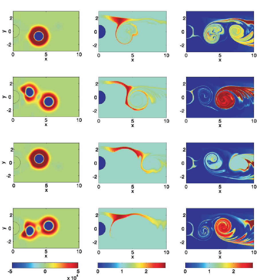
Figure 4 shows the average primary production (averaged over and then averaged in time) as a function of the vortex strength in the range . As anticipated, a transition from essentially no enrichment by the upwelling to an increasing primary production occurs around , confirming a direct influence of the physical transport process on the biological dynamics.
The dynamics in the low concentration inflow case is very different. For all values of considered, the average primary production in is smaller than the ambient one. This can be understood from the fact that fluid elements enter the domain with very low nutrient and plankton concentrations.
To better understand this situation we have performed numerical analysis of the NPZ dynamics without hydrodynamic terms. Figure 5 shows the time needed for and to reach their maximum values as a function of the initial conditions. We define as the fraction of the ambient concentrations that are present in the inflow: . With a mean flow of speed , fluid elements spend only days ( in units of ) inside the domain of horizontal extension in figure 1. We see in Fig. 5 that for the maximum in occurs later, so that we cannot expect considerable growth in outside the vortices for the value of used in this work. But this observation is also puzzling, since the primary production reported in figure 2 for the low inflow case is not as small as the above argument would indicate: It is reduced just between % and % with respect to the ambient values.
Figure 3 (right column) clarifies the mechanisms involved. The spatial plankton distribution is rather different from the ambient inflow case. It is clearly related to the vortices and associated structures. The plankton concentration is very low outside these objects. As in the case of ambient inflow, a plume with high nutrient concentration is present in the system due to upwelling and has a shape similar to the one in the ambient inflow case, which resembles the phytoplankton distribution of the central column of fig. 3, but here it seems to have no effect in inducing phytoplankton growth. The time scale for plankton growth starting from small values is much larger than the travel time through the computational area, thus these effects are observable only further downstream. Therefore, in the study area displayed in figures 1 and 3 the influence of the upwelling nutrient filament is masked by a more prominent mechanism, described below. In fact, in this low-inflow case, we note that the phenomenology observed in the area remains qualitatively unchanged if the upwelling is removed, although quantitative changes occur. This indicates that the dominant mechanism in the low inflow situation is not the mixing of upwelling and ambient waters, as in the ambient inflow situation, but the interaction of the inflow with the wake.


Figure 3 shows that phytoplankton growth in the vortices occurs after phytoplankton is transported into their interior by filaments emerging from the boundary of the circular obstacle. This complex structure – boundary of the obstacle, filaments emerging from it and rolling up around vortices – is well known from dynamical systems studies of this kind of flow (Jung et al., 1993; Ziemniak et al., 1994; Károlyi et al., 2000; Tél et al., 2005; Sandulescu et al., 2006), and is related to the so-called unstable manifold of the chaotic saddle, the main dynamical structure in the wakes occurring in time-dependent two-dimensional open flows. Loosely speaking, it is the location of the fluid elements that take a long time to leave the proximity of the island, because of the complex recirculation emerging just behind the obstacle as well as the reduced velocities occurring near its boundary. A detailed analysis of these structures and their implications for the residence times has been published in Sandulescu et al. (2007). Particle release calculations allow us to realize that, although most of the incoming particles follow the mean flow and leave the system in the days lapse estimated before, a fraction of them are captured by the wake structures with residence times of about to days for and , respectively. These long residence times allow the plankton concentration to build up in the filaments emerging from the obstacle, which gives rise to a plankton bloom later downstream, when the filaments are stretched and rolled up by the vortices.
Thus, recirculating structures in the island wake act as incubators that make fluid elements more productive before releasing them into the main current. It turns out that the peak values of the phytoplankton bloom in this low inflow case are larger than the ones under ambient inflow. This somehow paradoxical observation is explained by the fact that zooplankton values are relatively high under equilibrium ambient conditions, so that grazing control of the phytoplankton population is rather effective. By contrast, in the low inflow case zooplankton and thus grazing control is essentially absent. Zooplankton concentration begins to build up only when phytoplankton concentration has already reached larger values. Therefore it is responsible for the end of the bloom further downstream, but high phytoplankton values are attained before that.
Figure 2 (two lower curves) shows the time evolution of the primary production under the low inflow conditions. Even for , for which the wake acts as a barrier blocking nutrient fertilization of from the upwelling, primary production shows an oscillating behavior, reflecting the oscillations of the wake structure which is the responsible for the plankton growth. Figure 4 shows the increase in primary production by increasing the vortex strength starting at a value of . In the range of considered there is an increase in primary production by a factor of about , larger than the factor of increase attained under ambient inflow.
So far we have described two very distinct inflow situations and studied the impact of vortices by varying the vortex strength. We now fix the vortex strength to the high, , and low, , values, and describe the primary production behavior for intermediate inflow cases in figure 6 (solid line is for and dashed line for ). The inflow concentrations are now varied in terms of which, as already mentioned, gives the fraction of the ambient concentrations that are present in the inflow. For we have the low inflow conditions considered before, and corresponds to ambient input. We see, for both values of , an increase of the average production in with the biological content of the inflow, which is rather fast until .
Maximum values of the averages of and in are shown in Fig.7 for different initial conditions, with and without flow (i.e. in the spatially homogeneous case). It is seen a contrasting behavior remarking the fact that the flow is not simply redistributing biological material, but that it modifies also the spatial averages and then the total amounts of substances, as well as the qualitative dependence on . The large overshoots of the homogeneous case for low only occur inside vortices in the presence of flow, as will be discussed in the next section, so that the spatially averaged values of and are lower (see also Fig. 2). When approaching (the ambient inflow case), the relative increase in the presence of flow arises by advection from the upwelling plume.

For completeness, we present in Fig.8 the effect of reducing the effective diffusion . Physically this would mean that we decrease the intensity of small scale turbulence. We see that in general primary production is slightly reduced. The increase which is observed at low values of in the low inflow case is due to the lack of dilution of the filaments which emerge from the cylinder boundary. For the ambient inflow situation a small decrease of productivity for smaller is seen only at large vorticity, because distributions in are rather homogeneous otherwise.

3.2 Vortices and plankton distribution
It is well known that vortices are responsible for a large part of the transport and mixing phenomena at mesoscale on the ocean surface (Barton et al., 1998; Pelegrí et al., 2005; Martin et al., 2002). They influence biological dynamics, and most of the studies have focused on the effect of the relatively large vertical motions induced by their cores. Here we focus instead on horizontal processes. In this section we consider the case , where strong vortices are present in the system, and characterize the plankton distributions relative to vortex positions for the two different inflow conditions, that highlight the two different primary production enhancement mechanisms discussed above. Similar results are expected for other values of .
We make use of the Okubo-Weiss parameter (Okubo, 1970; Weiss, 1991) (a precise definition is included in the Appendix B) to identify in an objective way the interior and the exterior part of vortices. Flow regions with are vorticity dominated, and can be identified as the inner part of vortices. Regions with are strain dominated and outside vortices. The leftmost column of figure 3 displays the values, showing clearly the position of the vortices. These positions can be correlated with the phytoplankton distributions displayed in the other columns.

Figure 9 shows the spatial average of phytoplankton concentrations and primary production inside each of the two vortices and outside them. These regions are identified with the help of the Okubo-Weiss parameter . The primary production time series is qualitatively similar to the phytoplankton one, although slightly shifted towards earlier times. This is so because contains the influence of the nutrient dynamics, whose temporal evolution anticipates the phytoplankton one. The zooplankton time series (not shown) are also qualitatively similar but shifted towards later times.
In the case of ambient inflow the interior of the vortices (dashed and continuous lines) contains the same quantity of plankton as the inflow, namely the ambient concentration. Only when additional nutrients from the upwelling zone are entrained we observe bursts localized in time. Thus most of the biological activity is in the outside area (which includes the upwelling zone). This quantifies what is seen in the middle column of figure 3: plankton appears mainly in filaments that wind around the vortex periphery basically without entering them. The asymmetry observed between the content of the two vortices arises from the fact that, due to the different sense of rotation of the vortices more nutrients are transported towards the vicinity of the lower vortex than to the upper one (cf. figure 3).
The situation is rather different in the low inflow case. The range of the concentration oscillations is now larger, and the content of the two vortices oscillates in antiphase. The largest concentration values occur now inside vortex cores, leading to peak bloom values larger than for the ambient inflow situation. Minima are also smaller so that averages in regions such as give an overall smaller plankton content and primary production. Filamental structures close to the boundary of the island transport concentrations towards the vortices where the species are trapped and transported downstream. During this motion their concentrations are homogenized by small scale turbulence (modeled by the diffusion term in Eq. 3) and the classical dynamics that the system of equations (1) exhibits in a homogeneous situation occurs: nutrient consumption by phytoplankton induces a large phytoplankton bloom which is stopped by the grazing by zooplankton, that also experiences growth, until all three components approach the final equilibrium value . This steady state for the vortex content occurs only further downstream.
4 Conclusions
We have presented numerical results on the biological dynamics in the wake of an island close to a coastal upwelling area. Parameter values were appropriate for the Canary Islands region but we expect our results to be of greater generality.
Two different scenarios have been identified and discussed. In the first one, occurring when the region outside the focus area has properties similar to it, we have identified an enrichment mechanism of one side of the wake by nutrients upwelled on the other side. It occurs at sufficiently high vortex strength of the vortices present in the wake. Vortices entrain water from one side of the island in the form of filaments that are transported across the wake. Filaments of this type are observed in satellite images of the Canary area (Barton et al., 1998; Pelegrí et al., 2005). When the vortex strength is low, the wake acts rather as a barrier that blocks transport from one side to the other. This scenario is a direct translation of the behavior of passive tracers under similar flow (Sandulescu et al., 2006). We have also observed that a large decreasing of the eddy diffusion coefficient value has no relevant role in the primary productivity, though in general this is slightly reduced.
The second scenario becomes evident when the waters surrounding the study area are biologically much poorer. Now fertilization by the upwelling is not relevant, but we have identified a mechanism for primary production increase in the wake: The large residence times of some of the fluid particles in particular structures of the island wake allow them to become enriched by the ambient nutrient sources. Filaments from the wake structures feed this enriched water into the vortices, and the nonequilibrium plankton dynamics there leads to strong plankton blooms confined inside the vortices. The biological significance of hydrodynamical structures in the wake of obstacles has been recognized before (Károlyi et al., 2000; Scheuring et al., 2000; Tél et al., 2005), but in these cases the relevance was associated with their complex geometric structure that allowed fine intertwining of filaments containing different species or substances. The mechanism presented here seems to be different and simply associated with large residence times in the wake, leading to a kind of incubatory effect. A carefull study of the role of the different timescales present in the system has been presented in Sandulescu et al. (2007). We expect this mechanism to be at work in many types of island wakes, even if they are not associated with upwelling systems.
5 Acknowledgements
The authors thank T. Tél for many inspiring discussions. M.S. and U.F. acknowledge financial support by the DFG grant FE 359/7-1. E.H-G. and C.L. acknowledge financial support from MEC (Spain) and FEDER through projects CONOCE2 (FIS2004-00953) and FISICOS (FIS2007-60327), and from the PIF project OCEANTECH from CSIC. Both groups have benefited from a MEC-DAAD joint program.
Appendix A Numerical Algorithm
The coupling of the biological and the hydrodynamic model yields an advection-reaction-diffusion system. This system is numerically solved by a semi-Lagrangian algorithm. The concentrations of , and are represented on a grid of [500 x 300] points. The three processes, advection, reaction and diffusion, are performed sequentially as follows:
- •
Advection: Every point of the grid is integrated backwards in time with the velocity field for a time step . In this way we obtain the past position of the chosen point, which typically is not on the grid.
- •
Reaction: the concentration of , , or at the position obtained in the advection step is computed using a bilinear interpolation of its corresponding nearest points on the grid. Then these concentrations are the starting values for the integration of the reaction dynamics forward-in-time for a time step . In this way, we obtain the concentration of , and in the original grid point.
- •
Diffusion: Once we have the values of the concentrations on the grid, the diffusion step is performed following an Eulerian scheme. However, the interpolation in the reaction part induces a numerical diffusion of the order . It is therefore desirable to ensure that the real diffusion, which is given by the Okubo estimation (Okubo, 1971), is larger than this numerical diffusion. Moreover, the stability condition for the Eulerian diffusion step requires that , where denotes the time step for the diffusion part. These two inequalities are fullfilled if the diffusion time step is smaller than . According to this condition we chose in our algorithm. This implies that the algorithm makes ten steps of diffusion after every step of advection and reaction. Expressed in units of for time and for space, the dimensionless numerical values of the parameters are , , , and .
Appendix B The Okubo-Weiss parameter
The Okubo-Weiss parameter Okubo (1970); Weiss (1991) is a quantity used to distinguish areas in which the flow is dominated by vorticity from those areas where the flow is strain dominated. It is given by
| (4) |
where , are the normal and the shear components of strain, and is the relative vorticity of the flow defined as:
| (5) |
Where and are the horizontal components of the velocity field. We chose the critical threshold value to be . For areas where is below the flow is vortex dominated, otherwise we consider the flow to be strain dominated.
References
- Abraham (1998) Abraham, E.R. 1998 The generation of plankton patchiness by turbulent stirring. Nature 391, 577–580.
- Barton et al. (1998) Barton, E.D., Arístegui, J., Tett, P., Cantón, M., García-Braun, J., Hernández-León, S., Nykjaer, L., Almeida, C., Almunia, J., Ballesteros, S., Basterretxea, G., Escánez, J., García-Weill, L., Hernández-Guerra, A., López-Laatzen, F., Molina, R., Montero, M.F., Navarro-Pérez, E., Rodríguez, J.M., van Lenning, K., Vélez, H. & Wild, K. 1998 The transition zone of the canary current upwelling region. Progress in Oceanography 41, 455–504.
- Bracco et al. (2000) Bracco, A., Provenzale, A. & Scheuring, I. 2000 Mesoscale vortices and the paradox of the plankton. Proc. Roy. Soc. Lond. B 267, 1795–1800.
- Denman & Gargett (1995) Denman, K.L. & Gargett, A.E. 1995 Biological-physical interactions in the upper ocean: the role of vertical and small scale transport processes. Annu. Rev. Fluid Mech. 27, 225–255.
- Edwards & Brindley (1996) Edwards, M. & Brindley, J. 1996 Oscillatory behavior in a three-component plankton population model. Dyn. Stab. Sys. 11, 397–370.
- Hernández-García et al. (2002) Hernández-García, E., López, C. & Neufeld, Z. 2002 Small-scale structure of nonlinearly interacting species advected by chaotic flows. Chaos 12, 470–480.
- Hernández-García et al. (2003) Hernández-García, E., López, C. & Neufeld, Z. 2003 Spatial patterns in chemically and biologically reacting flows. In Chaos in Geophysical Flows (eds. G. Bofetta, G. Lacorata, G. Visconti & A. Vulpiani). Torino: OTTO Editore.
- Jung et al. (1993) Jung, C., Tél, T. & Ziemniak, E. 1993 Application of scattering chaos to particle transport in a hydrodynamical flow. Chaos 3, 555–568.
- Károlyi et al. (2000) Károlyi, G., Péntek, Á., Scheuring, I., Tél, T. & Toroczkai, Z. 2000 Chaotic flow: the physics of species coexistence. Proc. Natl. Acad. Sci. USA 97, 13661–13665.
- López et al. (2001a) López, C., Hernández-García, E., Piro, O., Vulpiani, A. & Zambianchi, E. 2001a Population dynamics advected by chaotic flows: A discrete-time map approach. Chaos 11, 397–403.
- López et al. (2001b) López, C., Neufeld, Z., Hernández-García, E. & Haynes, P.H. 2001b Chaotic advection of reacting substances: Plankton dynamics on a meandering jet. Phys. Chem. Earth B 26, 313–317.
- Mann & Lazier (1991) Mann, K.H. & Lazier, J.R.N. 1991 Dynamics of marine ecosystems. Biological-physical interactions in the oceans. Boston: Blackwell Scientific Publications.
- Martin (2003) Martin, A.P. 2003 Phytoplankton patchiness: the role of lateral stirring and mixing. Progress in Oceanography 57, 125–174.
- Martin et al. (2002) Martin, A.P., Richards, K.J., Bracco, A. & Provenzale, A. 2002 Patchy productivity in the open ocean. Global Biogeochemical Cycles 16, 10.1029/2001GB001449.
- Okubo (1970) Okubo, A. 1970 Horizontal dispersion of floatable particles in the vicinity of velocity singularities such as convergences. Deep-Sea Res. 17, 445–454.
- Okubo (1971) Okubo, A. 1971 Oceanic diffusion diagrams. Deep-Sea Res. 18, 789.
- Oschlies & Garçon (1999) Oschlies, A. & Garçon, V. 1999 An eddy-permitting coupled physical-biological model of the north-atlantic, sensitivity to advection numerics and mixed layer physics. Global Biocheochem. Cycles 13, 135–160.
- Pasquero et al. (2004) Pasquero, C., Bracco, A. & Provenzale, A. 2004 Coherent vortices, lagrangian particles and the marine ecosystem. In Shallow Flows (eds. W.S.J. Uijttewaal & G.H. Jirka). Leiden: Balkema Publishers, pp. 399–412.
- Pasquero et al. (2005) Pasquero, C., Bracco, A. & Provenzale, A. 2005 Impact of spatiotemporal variability of the nutrient flux on primary productivity in the ocean. J. Geophys. Res. 110, C07005.
- Pelegrí et al. (2005) Pelegrí, J.L., Arístegui, J., Cana, L., González-Dávila, M., Hernández-Guerra, A., Hernández-León, S., Marrero-Díaz, A., Montero, M.F., Sangrà, P. & Santana-Casiano, M. 2005 Coupling between the open ocean and the coastal upwelling region off northwest africa: Water recirculation and offshore pumping of organic matter. J. Mar. Sys. 54, 3–37.
- Peters & Marrasé (2000) Peters, F. & Marrasé, C. 2000 Effects of turbulence on plankton: an overview of experimental evidence and some theoretical considerations. Mar. Ecol. Prog. Ser. 205, 291–306.
- Reigada et al. (2003) Reigada, R., Hillary, R.M., Bees, M.A., Sancho, J.M. & Sagués, F. 2003 Plankton blooms induced by turbulent flows. Proc. Roy. Soc. Lond B 270, 875–880.
- Sandulescu et al. (2006) Sandulescu, M., Hernández-García, E., López, C. & Feudel, U. 2006 Kinematic studies of transport across an island wake, with application to the Canary islands. Tellus 58A, 605–615.
- Sandulescu et al. (2007) Sandulescu, M., López, C., Hernández-García, E. & Feudel, U. 2007 Plankton blooms in vortices: the role of biological and hydrodynamic timescales. Nonlinear Processes in Geophysics 14, 443–454.
- Scheuring et al. (2000) Scheuring, I., Károlyi, G., Péntek, Á., Tél, T. & Toroczkai, Z. 2000 A model for resolving the plankton paradox: coexistence in open flows. Freshwater Biol. 45, 123–132.
- Tél et al. (2005) Tél, T., de Moura, A., Grebogi, C. & Károlyi, G. 2005 Chemical and biological activity in open flows: A dynamical system approach. Phys. Rep. 413, 91–196. Erratum: Phys. Rep. 415, 360 (2005).
- Weiss (1991) Weiss, J 1991 The dynamics of enstrophy transfer in two-dimensional hydrodynamics. Physica D 48, 273–294.
- Ziemniak et al. (1994) Ziemniak, E., Jung, C. & Tél, T. 1994 Tracer dynamics in open hydrodynamical flows as chaotic scattering. Physica D 76, 123–146. Erratum in Physica D 79 (1994), 424.