跳到论文正文
W Papers独立论文阅读器 arXiv:0802.3473 论文正文 计算阅读时间 · 0%
引用这篇论文根据当前论文元数据生成,正式投稿前建议核对。


License: arXiv.org perpetual non-exclusive license
arXiv:0802.3473v2 [math.CO] 02 Apr 2009

On Cobweb Posets and Discrete F-Boxes Tilings

M. Dziemiańczuk
Abstract

FF-boxes defined in [6] as hyper-boxes in N∞N^{\infty} discrete space were applied here for the geometric description of the cobweb posetes Hasse diagrams tilings. The FF-boxes edges sizes are taken to be values of terms of natural numbers’ valued sequence FF. The problem of partitions of hyper-boxes represented by graphs into blocks of special form is considered and these are to be called FF-tilings.

The proof of such tilings’ existence for certain sub-family of admissible sequences FF is delivered. The family of FF-tilings which we consider here includes among others FF = Natural numbers, Fibonacci numbers, Gaussian integers with their corresponding FF-nomial (Binomial, Fibonomial, Gaussian) coefficients as it is persistent typical for combinatorial interpretation of such tilings originated from Kwaśniewski cobweb posets tiling problem .

Extension of this tiling problem onto the general case multi FF-nomial coefficients is here proposed. Reformulation of the present cobweb tiling problem into a clique problem of a graph specially invented for that purpose - is proposed here too. To this end we illustrate the area of our reconnaissance by means of the Venn type map of various cobweb sequences families.

AMS Classification Numbers: 05A10, 05A19, 11B83, 11B65

Keywords: partitions of discrete hyper-boxes, cobweb tiling problem, multi F-nomial coefficients

Affiliated to The Internet Gian-Carlo Polish Seminar:
http://ii.uwb.edu.pl/akk/sem/sem_rota.htm,
Article No7, April 2009, 15 April 2009,
(302 anniversary of Leonard Euler’s birth)

On Cobweb Posets
and Discrete F-Boxes Tilings

Maciej Dziemiańczuk

Institute of Informatics, University of Gdańsk
PL-80-952 Gdańsk, Wita Stwosza 57, Poland
e-mail: mdziemianczuk@gmail.com

1 Introduction

The Kwaśniewski upside-down notation from [4] (see also [1, 2]) is being here taken for granted. For example nn-th element of sequence FF is Fn≡nFF_{n}\equiv n_{F}, consequently nF!=nF⋅(n−1)F⋅…⋅1Fn_{F}!=n_{F}\cdot(n-1)_{F}\cdot...\cdot 1_{F} and a set [nF]={1,2,…,nF}[n_{F}]=\{1,2,...,n_{F}\} however [n]F={1F,2F,…,nF}[n]_{F}=\{1_{F},2_{F},...,n_{F}\}. More about effectiveness of this notation see references in [4] and Appendix “On upside-down notation” in [6].

Throughout this paper we shall consequently use FF letter for a sequence of positive integers i.e. F≡{nF}n≥0F\equiv\{n_{F}\}_{n\geq 0} such that nF∈ℕn_{F}\in\mathbb{N} for any n∈ℕ∪{0}n\in\mathbb{N}\cup\{0\}.

1.1 Discrete mm-dimensional FF-Box

Let us define discrete mm-dimensional FF-box with edges sizes designated by natural numbers’ valued sequence FF as described below. These FF-boxes from [6] where invented as a response to Kwaśniewski cobweb tiling problem posed in [1] (Problem 2 therein) and his question about visualization of this phenomenon.

Definition 1

Let FF be a natural numbers’ valued sequence {nF}n≥0\{n_{F}\}_{n\geq 0} and m,n∈ℕm,n\in\mathbb{N} such that n≥mn\geq m. Then a set Vm,nV_{m,n} of points v=(v1,…,vm)v=(v_{1},...,v_{m}) of discrete mm-dimensional space ℕm\mathbb{N}^{m} given as follows

Vm,n=[kF]×[(k+1)F]×…×[nF]V_{m,n}=[k_{F}]\times[(k+1)_{F}]\times...\times[n_{F}] (1)

where k=n−m+1k=n-m+1 and [sF]={1,2,…,sF}[s_{F}]=\{1,2,...,s_{F}\} is called mm-dimensional FF-box.

Refer to caption
Figure 1: FF-Boxes V2,3V_{2,3} and V3,4V_{3,4} with sub-boxes.

In the case of n=mn=m we write for short Vm,m≡VmV_{m,m}\equiv V_{m}. Assume that we have a mm-dimensional box Vm,n=W1×W2×…×WmV_{m,n}=W_{1}\times W_{2}\times...\times W_{m}. Then a set A=A1×A2×…×AmA=A_{1}\times A_{2}\times...\times A_{m} such that

As⊂Ws,|As|>0,s=1,2,…,m;A_{s}\subset W_{s},\qquad|A_{s}|>0,\qquad s=1,2,...,m;

is called mm-dimensional sub-box of Vm,nV_{m,n}. Moreover, if for s=1,2,…,ms=1,2,...,m these sets AsA_{s} satisfy the following

|As|=(σ⋅s)F|A_{s}|=(\sigma\cdot s)_{F}

for any permutation σ\sigma of set {1F,2F,…,mF}\{1_{F},2_{F},...,m_{F}\} then AA is called mm-dimensional sub-box of the form σ​Vm\sigma V_{m}. Compare with Figure 6.

Note, that the permutation σ\sigma might be understood here as an orientation of sub-box’s position in the box Vm,nV_{m,n}. Any two sub-boxes AA and BB are disjoint if its sets of points are disjoint i.e. A∩B=∅A\cap B=\emptyset.

The number of points v=(v1,…,vm)v=(v_{1},...,v_{m}) of mm-dimensional box Vm,nV_{m,n} is called volume. It it easy to see that the volume of Vm,nV_{m,n} is equal to

|Vm,n|=nF⋅(n−1)F⋅…⋅(n−m+1)F=nFm¯|V_{m,n}|=n_{F}\cdot(n-1)_{F}\cdot...\cdot(n-m+1)_{F}=n^{\underline{m}}_{F} (2)

while for m=nm=n

|Vm|=|σ​Vm|=mF⋅(m−1)F⋅…⋅1F=mF!|V_{m}|=|\sigma V_{m}|=m_{F}\cdot(m-1)_{F}\cdot...\cdot 1_{F}=m_{F}! (3)

1.2 Partition of discrete FF-boxes

Let us consider mm-dimensional FF-box Vm,nV_{m,n}. A finite collection of λ\lambda pairwise disjoint sub-boxes B1,B2,…,BλB_{1},B_{2},...,B_{\lambda} of the volume equal to κ\kappa is called κ\kappa-partition of Vm,nV_{m,n} if their set union of gives the whole box Vm,nV_{m,n} i.e.

⋃1≤j≤λBj=Vm,n,|Bi|=κ,i=1,2,…,λ.\bigcup_{1\leq j\leq\lambda}B_{j}=V_{m,n},\qquad|B_{i}|=\kappa,\qquad i=1,2,...,\lambda. (4)

Convention. In the following, we shall deal only with these κ\kappa-partition of mm-dimensional boxes Vm,nV_{m,n}, which volume κ\kappa of sub-boxes is equal to the volume of box VmV_{m} i.e. κ=|Vm|\kappa=|V_{m}|.

Of course the box Vm,nV_{m,n} has κ\kappa-partition not for all FF - sequences [8]. Therefore we introduce the name: FF-admissible sequence which means that FF satisfies the necessary and sufficient conditions for the box Vm,nV_{m,n} to have κ\kappa-partitions. In order to proceed let us recall first what follows.

Definition 2 ([1, 2])

Let FF be a natural numbers’ valued sequence F={nF}n≥0F=\{n_{F}\}_{n\geq 0}. Then FF-nomial coefficient is identified with the symbol

(nm)F=nF!mF!​(n−m)F!=nFm¯mF!{{n}\choose{m}}_{\!\!F}=\frac{n_{F}!}{m_{F}!(n-m)_{F}!}=\frac{n_{F}^{\underline{m}}}{m_{F}!} (5)

where nF0¯=0F!=1n_{F}^{\underline{0}}=0_{F}!=1.

Definition 3 ([1, 2])

A sequence FF is called admissible if, and only if for any n,m∈ℕ∪{0}n,m\in\mathbb{N}\cup\{0\} the value of FF-nomial coefficient is natural number or zero i.e.

(nm)F∈ℕ∪{0}{{n}\choose{m}}_{\!\!F}\in\mathbb{N}\cup\{0\} (6)

while n≥mn\geq m else is zero.

Recall now also a combinatorial interpretation of the FF-nomial coefficients in FF-box reformulated form (consult Remark 5 in [4] and [6]). And note: these coefficients encompass among others Binomial, Gaussian and Fibonomial coefficients.

Fact 1 (Kwaśniewski [1, 2])

Let FF be an admissible sequence. Take any m,n∈ℕm,n\in\mathbb{N} such that n≥mn\geq m, then the value of FF-nomial coefficient (nm)F{{n}\choose{m}}_{\!\!F} is equal to the number of sub-boxes that constitute a κ\kappa-partition of mm-dimensional FF-box Vm,nV_{m,n} where κ=|Vm|\kappa=|V_{m}|.

Proof. This proof comes from Observation 3 in [1, 2] and was adopted here to the language of discrete boxes. Let us consider mm-dimensional box Vm,nV_{m,n} with |Vm,n|=nFm¯|V_{m,n}|=n^{\underline{m}}_{F}. The volume of sub-boxes is equal to κ=|Vm|=mF!\kappa=|V_{m}|=m_{F}!. Therefore the number of sub-boxes is equal to

nFm¯mF!=(nm)F\frac{n^{\underline{m}}_{F}}{m_{F}!}={{n}\choose{m}}_{\!\!F}

From definition of FF-admissible sequence we have that the above is natural number. Hence the thesis ■\blacksquare

While considering any κ\kappa-partition of certain mm-dimensional box we only assume that sub-boxes have the same volume. In the next section we shall take into account these partitions which sub-boxes have additionally established structure.

1.3 Tiling problem

Now, special κ\kappa-partitions of discrete boxes are considered. Namely, we deal with only these partitions of mm-dimensional box Vm,nV_{m,n} which all sub-boxes are of the form VmV_{m}.

Definition 4

Let Vm,nV_{m,n} be a mm-dimensional FF-box. Then any κ\kappa-partition into sub-boxes of the form VmV_{m} is called tiling of Vm,nV_{m,n}.

It was shown in [8] that just the admissibility condition (6) is not sufficient for the existence a tiling for any given mm-dimensional box Vm,nV_{m,n}. Kwaśniewski in his papers [1, 2] posed the following problem called Cobweb Tiling Problem, which was a starting point of the research with results being reported in the presents note.

Problem 1 (Tiling)

Suppose now that FF is an admissible sequence. Under which conditions any FF-box Vm,nV_{m,n} designated by sequence FF has a tiling? Find effective characterizations and/or find an algorithm to produce these tilings.

Refer to caption
Figure 2: Sample 3D and 2D tilings.

In the next sections we propose certain family 𝒯λ\mathcal{T}_{\lambda} of sequences FF. Then we prove that any FF-box Vm,nV_{m,n}, where m,n∈ℕm,n\in\mathbb{N} designated by F∈𝒯λF\in\mathcal{T}_{\lambda} has a tiling with giving a construction of it.

1.4 Cobweb representation

In this section we recall [6] that discrete FF-boxes Vm,nV_{m,n} are unique codings representing Cobwebs, introduced by Kwaśniewski [1, 2] as a special graded posets. Any poset might be represented as a Hasse digraph and this approach to tiling problem will be used throughout the paper.

Next we shall consider partitions of mm-dimensional boxes as a partitions of cobwebs with mm levels into sub-cobwebs called blocks. In the following we quote some necessary notation of Cobwebs adopted to the tiling problem. For more on Cobwebs see source papers [1, 2, 4] and references therein.

Definition 5

Let FF be a natural numbers’ valued sequence. Then a simple graph ⟨V,E⟩\langle V,E\rangle, such that V=⋃k≤s≤nΦsV=\bigcup_{k\leq s\leq n}\Phi_{s} and

E={{u,v}:u∈Φs∧v∈Φs+1∧k≥s<n}E=\Big\{\{u,v\}:u\in\Phi_{s}\wedge v\in\Phi_{s+1}\wedge k\geq s<n\Big\} (7)

where Φs={1,2,…,sF}\Phi_{s}=\{1,2,...,s_{F}\} is called cobweb layer ⟨Φk→Φn⟩\penalty{\langle\Phi_{k}\!\to\!\Phi_{n}\rangle}.

Refer to caption
Figure 3: Cobweb layer ⟨Φ2→Φ4⟩\penalty{\langle\Phi_{2}\!\to\!\Phi_{4}\rangle} designated by FF=Natural numbers.

Suppose that we have a cobweb layer ⟨Φk→Φn⟩\penalty{\langle\Phi_{k}\!\to\!\Phi_{n}\rangle} of mm levels Φs\Phi_{s}, where m=n−k+1m=n-k+1. Then any cobweb layer ⟨ϕ1→ϕm⟩\langle\phi_{1}\to\phi_{m}\rangle of mm levels ϕs\phi_{s} such that

ϕs⊆Φs,|ϕs|=sF,s=1,2,…,m;\phi_{s}\subseteq\Phi_{s},\qquad|\phi_{s}|=s_{F},\qquad s=1,2,...,m; (8)

is called cobweb block PmP_{m} of layer ⟨Φk→Φn⟩\penalty{\langle\Phi_{k}\!\to\!\Phi_{n}\rangle}.

Additionally, one considers cobweb blocks obtained via permutation σ\sigma of theirs levels’ order as follows (Compare with Figure 4).

Refer to caption
Figure 4: Example of cobweb blocks P3P_{3} and σ​P3\sigma P_{3}.
Definition 6

Let a cobweb layer ⟨Φk→Φn⟩\penalty{\langle\Phi_{k}\!\to\!\Phi_{n}\rangle} with mm levels Φs\Phi_{s} be given, where m=n−k+1m=n-k+1. Then a cobweb block PmP_{m} with mm levels ϕs\phi_{s} such that

ϕs⊆Φs,|ϕs|=(σ⋅s)F,s=1,2,…,m;\phi_{s}\subseteq\Phi_{s},\qquad|\phi_{s}|=(\sigma\cdot s)_{F},\qquad s=1,2,...,m; (9)

where σ\sigma is a permutation of the set {1F,2F,…,mF}\{1_{F},2_{F},...,m_{F}\} is called cobweb block of the form σ​Pm\sigma P_{m}.

Refer to caption
Figure 5: FF-Boxes of the form σ​V2\sigma V_{2} and cobweb blocks σ​P2\sigma P_{2}.

While saying “a block σ​Pm\sigma P_{m} of layer ⟨Φk→Φn⟩\penalty{\langle\Phi_{k}\!\to\!\Phi_{n}\rangle}” we mean that the number of levels in block and layer is the same i.e. m=n−k+1m=n-k+1 and each of levels of block are non-empty subsets of corresponding levels in the layer.

Assume that we have a cobweb layer ⟨Φk→Φn⟩\penalty{\langle\Phi_{k}\!\to\!\Phi_{n}\rangle}. A path π\pi from any vertex at first level Φk\Phi_{k} to any vertex at the last level Φn\Phi_{n}, such that

π={vk,vk+1,…,vn},vs∈Φs,s=k,k+1,…,n;\pi=\{v_{k},v_{k+1},...,v_{n}\},\qquad v_{s}\in\Phi_{s},\qquad s=k,k+1,...,n;

is noted as a maximal-path π\pi of ⟨Φk→Φn⟩\penalty{\langle\Phi_{k}\!\to\!\Phi_{n}\rangle}. In the same way we nominate maximal-path of cobweb block σ​Pm\sigma P_{m}.

Let Cm​a​x​(A)C_{max}(A) denotes a set of maximal-paths π\pi of cobweb block AA. (Compare with [4]). Two cobweb blocks A,BA,B of layer ⟨Φk→Φn⟩\penalty{\langle\Phi_{k}\!\to\!\Phi_{n}\rangle} are max-disjoint or disjoint for short ([1, 2]) if, and only if its sets of maximal-paths are disjoint i.e. Cm​a​x​(A)∩Cm​a​x​(B)=∅C_{max}(A)\cap C_{max}(B)=\emptyset. The cardinality of set Cm​a​x​(A)C_{max}(A) is called size of block AA.

Refer to caption
Figure 6: FF-Boxes of the form σ​V3\sigma V_{3} and cobweb blocks σ​P3\sigma P_{3}.
Observation 1 ([6])

Let FF be a natural numbers’ valued sequence and k,n∈ℕk,n\in\mathbb{N}. Then any FF-box Vm,nV_{m,n} is uniquely represented by cobweb layer ⟨Φk→Φn⟩\penalty{\langle\Phi_{k}\!\to\!\Phi_{n}\rangle} and vice versa i.e.,

Vm,n⇔⟨Φk→Φn⟩.V_{m,n}\Leftrightarrow\penalty{\langle\Phi_{k}\!\to\!\Phi_{n}\rangle}. (10)

where k=n−m+1k=n-m+1.

Proof. Consider a cobweb layer ⟨Φk→Φn⟩\penalty{\langle\Phi_{k}\!\to\!\Phi_{n}\rangle} of mm levels Φ\Phi and mm-dimensional box Vk,nV_{k,n}. Observe that any maximal-path π=(v1,v2,…,vm)\pi=(v_{1},v_{2},...,v_{m}) of the layer corresponds to only one point x=(x1,x2,…,xm)x=(x_{1},x_{2},...,x_{m}) of mm-dimensional box Vm,nV_{m,n}, and vice versa, i.e.

[sF]∋xs⇔vs∈[sF],s=1,2,…,m;[s_{F}]\ni x_{s}\Leftrightarrow v_{s}\in[s_{F}],\qquad s=1,2,...,m;

And the number of these maximal-paths and points is the same (Compare with [4] and [6]) i.e.

|Cm​a​x​(⟨Φk→Φn⟩)|=|Vm,n||C_{max}(\penalty{\langle\Phi_{k}\!\to\!\Phi_{n}\rangle})|=|V_{m,n}|

where m=n−k+1m=n-k+1. ■\blacksquare

Refer to caption
Figure 7: Correspondence between tiling of FF-box V3,4V_{3,4} and ⟨Φ3→Φ4⟩\penalty{\langle\Phi_{3}\!\to\!\Phi_{4}\rangle}.

Next, we draw terminology of FF-boxes’ partitions back to cobweb’s language, used in the next part of this note.

Take any cobweb layer ⟨Φk→Φn⟩\penalty{\langle\Phi_{k}\!\to\!\Phi_{n}\rangle} with mm levels. Then a set of λ\lambda pairwise disjoint cobweb blocks A1,A2,…,AλA_{1},A_{2},...,A_{\lambda} of mm levels such that its size is equal to κ\kappa and the union of Cm​a​x​(A1),Cm​a​x​(A2),…,Cm​a​x​(Aλ)C_{max}(A_{1}),C_{max}(A_{2}),...,C_{max}(A_{\lambda}) is equal to the set Cm​a​x​(⟨Φk→Φn⟩)C_{max}(\penalty{\langle\Phi_{k}\!\to\!\Phi_{n}\rangle}) is called cobweb κ\kappa-partition. Finally, a κ\kappa-partition of layer ⟨Φk→Φn⟩\penalty{\langle\Phi_{k}\!\to\!\Phi_{n}\rangle} with mm levels into cobweb blocks of the form σ​Pm\sigma P_{m} is called cobweb tiling.

Let us sum it up with the following Table 1.

Table 1: Equivalent notation and terminology.
Cobwebs FF-boxes
1. Maximal-path (v1,…,vm)∈⟨Φk→Φn⟩(v_{1},...,v_{m})\in\penalty{\langle\Phi_{k}\!\to\!\Phi_{n}\rangle} Point (x1,…,xm)∈Vm,n(x_{1},...,x_{m})\in V_{m,n}
2. Cobweb layer ⟨Φk→Φn⟩\penalty{\langle\Phi_{k}\!\to\!\Phi_{n}\rangle} FF-box Vm,nV_{m,n}
3. Cobweb block σ​Pm⊂⟨Φk→Φn⟩\sigma P_{m}\subset\penalty{\langle\Phi_{k}\!\to\!\Phi_{n}\rangle} Sub-box σ​Vm⊂Vm,n\sigma V_{m}\subset V_{m,n}
4. Tiling of cobweb layer Tiling of FF-box
where k = n-m+1.

2 Cobweb tiling sequences

Recall that for some FF-admissible sequences there is no method to tile certain FF-boxes Vm,nV_{m,n} or accordingly cobweb layers ⟨Φk→Φn⟩\penalty{\langle\Phi_{k}\!\to\!\Phi_{n}\rangle} (no tiling property). For example see Figure 8 that comes from [8]. In the next part of this note, we define and consider only sequences with tiling property.

Refer to caption
Figure 8: Layer ⟨Φ5→Φ7⟩\penalty{\langle\Phi_{5}\!\to\!\Phi_{7}\rangle} that does not have tiling with blocks σ​P3\sigma P_{3}.
Definition 7

A cobweb admissible sequence FF such that for any m,n∈ℕm,n\in\mathbb{N} the cobweb layer ⟨Φk→Φn⟩\penalty{\langle\Phi_{k}\!\to\!\Phi_{n}\rangle} has a tiling is called cobweb tiling sequence.

Let 𝒯\mathcal{T} denotes the family of all cobweb tiling sequences. Characterization of whole family 𝒯\mathcal{T} is still open problem. Nevertheless we define certain subfamily 𝒯λ⊂𝒯\mathcal{T}_{\lambda}\subset\mathcal{T} of non-trivial cobweb tiling sequences. This family contains among others Natural and Fibonacci numbers, Gaussian integers and others.

Notation 1

Let 𝒯λ\mathcal{T}_{\lambda} denotes the family of natural number’s valued sequences F≡{nF}n≥1F\equiv\{n_{F}\}_{n\geq 1} such that for any nn-th term of FF satisfies the following holds

∀m,k∈ℕ,nF=(m+k)F=λK⋅kF+λM⋅mF\forall~m,k\in\mathbb{N},\quad n_{F}=(m+k)_{F}=\lambda_{K}\cdot k_{F}\ +\ \lambda_{M}\cdot m_{F} (11)

while 1F∈ℕ1_{F}\in\mathbb{N} and for certain coefficients λK≡λK​(k,m)∈ℕ∪{0}\lambda_{K}\equiv\lambda_{K}(k,m)\in\mathbb{N}\cup\{0\} and λM≡λM​(k,m)∈ℕ∪{0}\lambda_{M}\equiv\lambda_{M}(k,m)\in\mathbb{N}\cup\{0\}.

Note, coefficients λK\lambda_{K} and λM\lambda_{M} might be considered as a natural numbers’ with zero valued infinite matrixes λK≡[ki​j]i,j≥1\lambda_{K}\equiv[k_{ij}]_{i,j\geq 1} and λM≡[mi​j]i,j≥1\lambda_{M}\equiv[m_{ij}]_{i,j\geq 1}. Moreover the sequence F≡{nF}n≥0F\equiv\{n_{F}\}_{n\geq 0} is uniquely designated by these matrixes λK,λM\lambda_{K},\lambda_{M} and first element 1F∈ℕ1_{F}\in\mathbb{N}.

Corollary 1

Let a sequence F∈𝒯λF\in\mathcal{T}_{\lambda} with its coefficients’ matrixes λK,λM\lambda_{K},\lambda_{M} and a composition β→=⟨b1,b2,…,bk⟩\vec{\beta}=\langle b_{1},b_{2},...,b_{k}\rangle of number nn into kk nonzero parts be given. Then the following takes place

nF=1F​∑s=1nλs​(β→)⋅(bs)Fn_{F}=1_{F}\sum_{s=1}^{n}\lambda_{s}(\vec{\beta})\cdot(b_{s})_{F} (12)

where

λs​(β→)=λK​(bs,bs+1+…+bk)​∏i=1s−1λM​(bi,bi+1+…+bk)\lambda_{s}(\vec{\beta})=\lambda_{K}(b_{s},b_{s+1}+...+b_{k})\prod_{i=1}^{s-1}\lambda_{M}(b_{i},b_{i+1}+...+b_{k}) (13)

or equivalent

λs​(β→)=λM​(bs+1+…+bk,bs)​∏i=1s−1λK​(bi+1+…+bk,bi).\lambda_{s}(\vec{\beta})=\lambda_{M}(b_{s+1}+...+b_{k},b_{s})\prod_{i=1}^{s-1}\lambda_{K}(b_{i+1}+...+b_{k},b_{i}). (14)

Proof. It is a straightforward algebraic induction exercise using property (11) of the sequence 𝒯λ\mathcal{T}_{\lambda}. The first form (13) of the coefficients λs​(β→)\lambda_{s}(\vec{\beta}) comes from the following

(b1+(n−b1))F⇒(b1+b2+(n−b1−b2))F\Big(b_{1}+(n-b_{1})\Big)_{\!F}\Rightarrow\Big(b_{1}+b_{2}+(n-b_{1}-b_{2})\Big)_{\!F}

while the second one (14) from

((n−bk)+bk)F⇒((n−bk−bk−1)+bk−1+bk)F■\Big((n-b_{k})+b_{k}\Big)_{\!F}\Rightarrow\Big((n-b_{k}-b_{k-1})+b_{k-1}+b_{k}\Big)_{\!F}\qquad\blacksquare

If we take a vector ⟨1,1,…,1⟩\langle 1,1,...,1\rangle of nn ones i.e. bs=1b_{s}=1 for any s=1,2,…,ns=1,2,...,n; then we obtain alternative formula to compute elements of the sequence FF.

Corollary 2

Let F∈𝒯λF\in\mathcal{T}_{\lambda} be given. Then nn-th element of the sequence FF satisfies

nF=1F⋅∑s=1nλK​(1,n−s)​∏i=1s−1λM​(1,n−i)n_{F}=1_{F}\cdot\sum_{s=1}^{n}\lambda_{K}(1,n-s)\prod_{i=1}^{s-1}\lambda_{M}(1,n-i) (15)

for any n∈ℕn\in\mathbb{N}.

Corollary 3

Let any sequence F∈𝒯λF\in\mathcal{T}_{\lambda} be given. Then for any n,k∈ℕ∪{0}n,k\in\mathbb{N}\cup\{0\} such that n≥kn\geq k, the FF-nomial coefficients satisfy below recurrence identity

(nk)F=λK​(n−1k−1)F+λM​(n−1k)F{{n}\choose{k}}_{\!\!F}=\lambda_{K}{{n-1}\choose{k-1}}_{\!\!F}+\lambda_{M}{{n-1}\choose{k}}_{\!\!F} (16)

where (nn)F=(n0)F=1{n\choose n}_{F}={n\choose 0}_{F}=1.

Proof. Take any F∈𝒯λF\in\mathcal{T}_{\lambda} and n∈ℕ∪{0}n\in\mathbb{N}\cup\{0\}. Then from (11) of 𝒯λ\mathcal{T}_{\lambda} and for any m,k∈ℕ∪{0}m,k\in\mathbb{N}\cup\{0\} such that m+k=nm+k=n we have that nn-th element of the sequence FF satisfies following recurrence

nF=(k+m)F=λK⋅kF+λM⋅mFn_{F}=(k+m)_{F}=\lambda_{K}\cdot k_{F}+\lambda_{M}\cdot m_{F}

Multiply both sides of above equation by (n−1)F!kF!⋅mF!\frac{(n-1)_{F}!}{k_{F}!\cdot m_{F}!} to get

nF!kF!⋅mF!=λK⋅(n−1)F!(k−1)F!⋅mF!+λM⋅(n−1)F!kF!⋅(m−1)F!\frac{n_{F}!}{k_{F}!\cdot m_{F}!}=\lambda_{K}\cdot\frac{(n-1)_{F}!}{(k-1)_{F}!\cdot m_{F}!}+\lambda_{M}\cdot\frac{(n-1)_{F}!}{k_{F}!\cdot(m-1)_{F}!}

And from Definition 2 of FF-nomial coefficients we have

(nk)F=λK​(n−1k−1)F+λM​(n−1k)F■{{n}\choose{k}}_{\!\!F}=\lambda_{K}{n-1\choose k-1}_{F}+\lambda_{M}{{n-1}\choose{k}}_{\!\!F}\quad\blacksquare

It turns out that the recurrence formula (16) gives us a method to generating tilings of any layer ⟨Φk→Φn⟩\penalty{\langle\Phi_{k}\!\to\!\Phi_{n}\rangle} designated by sequence F∈𝒯λF\in\mathcal{T}_{\lambda}.

Theorem 1

Let FF be a sequence of 𝒯λ\mathcal{T}_{\lambda} family. Then FF is cobweb tiling.

Refer to caption
Figure 9: Picture of Theorem 1 proof’s idea.

Proof. Suppose that we have a cobweb layer ⟨Φk+1→Φn⟩\penalty{\langle\Phi_{k+1}\!\to\!\Phi_{n}\rangle} with mm levels designated by sequence FF from 𝒯λ\mathcal{T}_{\lambda} family and m=n−km=n-k. Consider Φn\Phi_{n} level with nFn_{F} vertices. From (11) we have that the number of vertices at this level is the sum of λM⋅mF\lambda_{M}\cdot m_{F} and λK⋅kF\lambda_{K}\cdot k_{F}. Therefore we separate them by cutting into two disjoint subsets as illustrated by Figure 9 and cope at first λM⋅mF\lambda_{M}\cdot m_{F} vertices in Step 1. Then we shall cope the rest λK⋅kF\lambda_{K}\cdot k_{F} ones in Step 2.

Refer to caption
Figure 10: Picture of Theorem 1 proof’s Step 1.

Step 1. Temporarily we have λM⋅mF\lambda_{M}\cdot m_{F} fixed vertices on Φn\Phi_{n} level to consider (Figure 10). Let us cover them λM\lambda_{M} times by mm-th level of block σ​Pm\sigma P_{m}, which has exactly mFm_{F} vertices. If λM=0\lambda_{M}=0 we skip this step. What was left is the layer ⟨Φk+1→Φn−1⟩\penalty{\langle\Phi_{k+1}\!\to\!\Phi_{n-1}\rangle} and we might eventually partition it with smaller disjoint blocks σ​Pm−1\sigma P_{m-1} in the next induction step .

Refer to caption
Figure 11: Picture of Theorem 1 proof’s Step 2.

Step 2. Consider now the second complementary situation, where we have λK⋅kF\lambda_{K}\cdot k_{F} vertices on Φn\Phi_{n} level being fixed (Figure 11). If λK=0\lambda_{K}=0 we skip this step. Observe that if we move this level lower than Φk+1\Phi_{k+1} level, we obtain exactly λK\lambda_{K} the same layers ⟨Φk→Φn−1⟩\penalty{\langle\Phi_{k}\!\to\!\Phi_{n-1}\rangle} to be partitioned with disjoint blocks of the form σ​Pm\sigma P_{m}. This “move” operation is just permutation σ\sigma of levels’ order.

Recapitulation. The layer ⟨Φk+1→Φn⟩\penalty{\langle\Phi_{k+1}\!\to\!\Phi_{n}\rangle} might be partitioned into σ​Pm\sigma P_{m} blocks if ⟨Φk+1→Φn−1⟩\penalty{\langle\Phi_{k+1}\!\to\!\Phi_{n-1}\rangle} might be partitioned into σ​Pm−1\sigma P_{m-1} and ⟨Φk→Φn−1⟩\penalty{\langle\Phi_{k}\!\to\!\Phi_{n-1}\rangle} into σ​Pm\sigma P_{m} again. Continuing these steps by induction, we are left to prove that ⟨Φk→Φk⟩\penalty{\langle\Phi_{k}\!\to\!\Phi_{k}\rangle} might be partitioned into σ​P1\sigma P_{1} blocks and ⟨Φ1→Φm⟩\penalty{\langle\Phi_{1}\!\to\!\Phi_{m}\rangle} into σ​Pm\sigma P_{m} ones, what is trivial ■\blacksquare

Observation 2

Let FF be a cobweb tiling sequence from the family 𝒯λ\mathcal{T}_{\lambda}. Then the number {nk}F1\Big\{{n\atop k}\Big\}_{F}^{1} of different tilings of layer ⟨Φk→Φn⟩\penalty{\langle\Phi_{k}\!\to\!\Phi_{n}\rangle} where n,k∈ℕn,k\in\mathbb{N}, n,k≥1n,k\geq 1 is equal to:

{nk}F1=nF!(mF!)λM⋅((k−1)F!)λK⋅({n−1k}F1)λM⋅({n−1k−1}F1)λK\bigg\{{n\atop{k}}\bigg\}_{F}^{1}=\frac{n_{F}!}{(m_{F}!)^{\lambda_{M}}\cdot((k-1)_{F}!)^{\lambda_{K}}}\cdot\bigg(\bigg\{{n-1\atop k}\bigg\}_{F}^{1}\bigg)^{\lambda_{M}}\cdot\bigg(\bigg\{{n-1\atop k-1}\bigg\}_{F}^{1}\bigg)^{\lambda_{K}} (17)

where {nn}F1=1\Big\{{n\atop n}\Big\}_{F}^{1}=1 and {n1}F1=1\Big\{{n\atop 1}\Big\}_{F}^{1}=1.

Proof. According to steps of the proof of Theorem 1 we might choose mFm_{F} vertices λM\lambda_{M} times at nn-th level and next (k−1)F(k-1)_{F} vertices λK\lambda_{K} times out of nFn_{F} ones in nF!(mF!)λM⋅((k−1)F!)λK\frac{n_{F}!}{(m_{F}!)^{\lambda_{M}}\cdot((k-1)_{F}!)^{\lambda_{K}}} ways. Next recurrent steps of the proof of Theorem 1 result in formula (17) via product rule of counting ■\blacksquare

Note that {nk}F1\Big\{{n\atop k}\Big\}_{F}^{1} is not the number of all different tilings of the layer ⟨Φk→Φn⟩\penalty{\langle\Phi_{k}\!\to\!\Phi_{n}\rangle} i.e. {nk}F1≤{nk}F\Big\{{n\atop k}\Big\}_{F}^{1}\leq\Big\{{n\atop k}\Big\}_{F} as computer experiments show [8]. There are much more other tilings with blocks σ​Pm\sigma P_{m}.

3 Cobweb multi tiling

In this section, more general case of the tiling problem is considered. For that to do we introduce the so-called multi FF-nomial coefficients that counts blocks of multi-block partitions.

Definition 8

Let natural numbers’ valued sequence F≡{nF}n≥0F\equiv\{n_{F}\}_{n\geq 0} and a composition ⟨b1,b2,…,bk⟩\langle b_{1},b_{2},...,b_{k}\rangle of the number nn be given. Then the multi FF-nomial coefficient is identified with the symbol

(nb1,b2,…,bk)F=nF!(b1)F!⋅…⋅(bk)F!{{n}\choose{b_{1},b_{2},...,b_{k}}}_{\!\!F}=\frac{n_{F}!}{(b_{1})_{F}!\cdot...\cdot(b_{k})_{F}!} (18)

while n=b1+b2+…+bkn=b_{1}+b_{2}+...+b_{k}.

Corollary 4

Let FF be any FF-cobweb admissible sequence. Then value of the multi FF-nomial coefficient is natural number or zero i.e.

(nb1,b2,…,bk)F∈ℕ∪{0}{{n}\choose{b_{1},b_{2},...,b_{k}}}_{\!\!F}\in\mathbb{N}\cup\{0\} (19)

for any n,b1,b2,…,bk∈ℕn,b_{1},b_{2},...,b_{k}\in\mathbb{N} such that n=b1+b2+…+bkn=b_{1}+b_{2}+...+b_{k}.

For the sake of forthcoming combinatorial interpretation of multi FF-nomial coefficients we introduce the following notation.

Definition 9

Let a cobweb layer ⟨Φ1→Φn⟩\penalty{\langle\Phi_{1}\!\to\!\Phi_{n}\rangle} of nn levels Φs\Phi_{s} and a composition ⟨b1,b2,…,bk⟩\langle b_{1},b_{2},...,b_{k}\rangle of number nn into kk non-zero parts be given. Then any cobweb layer ⟨ϕ1→ϕn⟩\langle\phi_{1}\to\phi_{n}\rangle of nn levels ϕs\phi_{s} such that

ϕs⊆Φs,s=1,2,…,n;\phi_{s}\subseteq\Phi_{s},\qquad s=1,2,...,n; (20)

where the cardinality of ϕs\phi_{s} is equal to ss-th element of the vector LL given as follows

L=σ⋅⟨1,2,…,b1,1,2,…,b2,…,1,2,…,bk⟩L=\sigma\cdot\langle 1,2,...,b_{1},1,2,...,b_{2},...,1,2,...,b_{k}\rangle

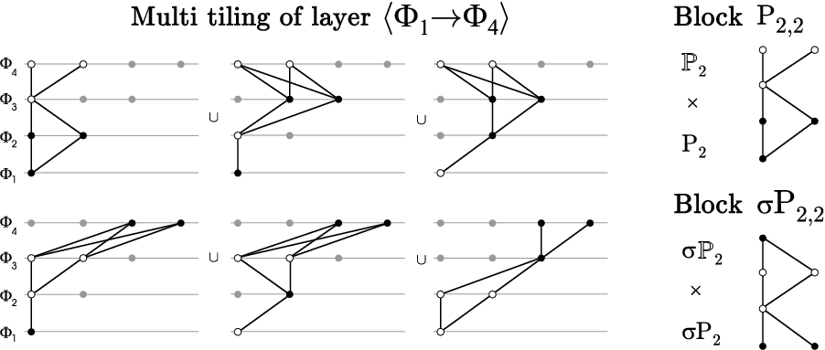
for any permutation σ\sigma of a set [n][n] is called cobweb multi-block of the form σ​Pb1,b2,…,bk\sigma P_{b_{1},b_{2},...,b_{k}}.

Refer to caption
Figure 12: Examples of multi blocks P4,2,1P_{4,2,1} and σ​P4,2,1\sigma P_{4,2,1}.

In the case of σ=i​d\sigma=id we write for short σ​Pb1,b2,…,bk=Pb1,b2,…,bk\sigma P_{b_{1},b_{2},...,b_{k}}=P_{b_{1},b_{2},...,b_{k}}. Compare with Figure 12.

Example 1
Take a sequence FF of next natural numbers i.e. nF=nn_{F}=n and cobweb layer ⟨Φ1→Φ4⟩\penalty{\langle\Phi_{1}\!\to\!\Phi_{4}\rangle} designated by FF. A sample multi tiling of the layer ⟨Φ1→Φ4⟩\penalty{\langle\Phi_{1}\!\to\!\Phi_{4}\rangle} with the help of (42,2)F=6{{4}\choose{2,2}}_{\!\!F}=6 disjoint multi blocks of the form σ​P2,2\sigma P_{2,2} is in Figure 13.

Refer to caption
Figure 13: Sample multi tiling of layer ⟨Φ1→Φ4⟩\penalty{\langle\Phi_{1}\!\to\!\Phi_{4}\rangle} from Example 2.
Observation 3

Let ⟨Φ1→Φn⟩\penalty{\langle\Phi_{1}\!\to\!\Phi_{n}\rangle} be a cobweb layer and ⟨b1,…,bk⟩\langle b_{1},...,b_{k}\rangle be a composition of the number nn into kk nonzero parts. Then the value of multi FF-nomial coefficient (nb1,b2,…,bk)F{{n}\choose{b_{1},b_{2},...,b_{k}}}_{\!\!F} is equal to the number of blocks that form the cobweb κ\kappa-partition, where κ=|Cm​a​x​(Pb1,…,bk)|\kappa=|C_{max}(P_{b_{1},...,b_{k}})|.

Proof. The proof is natural extension of Observation 3 in [1, 2]. The number of maximal paths in layer ⟨Φ1→Φn⟩\penalty{\langle\Phi_{1}\!\to\!\Phi_{n}\rangle} is equal to nF!n_{F}!. However the number of maximal paths in any multi block σ​Pb1,b2,…,bk\sigma P_{b_{1},b_{2},...,b_{k}} is (b1)F!⋅(b2)F!⋅…⋅(bk)F!\penalty{(b_{1})_{F}!\cdot(b_{2})_{F}!\cdot...\cdot(b_{k})_{F}!}. Thus the number of such blocks is equal to

nF!(b1)F!⋅(b2)F!⋅…⋅(bk)F!\frac{n_{F}!}{(b_{1})_{F}!\cdot(b_{2})_{F}!\cdot...\cdot(b_{k})_{F}!}

where n=b1+b2+…+bkn=b_{1}+b_{2}+...+b_{k} for any n,k∈ℕn,k\in\mathbb{N} ■\blacksquare

Of course for k=2k=2 we have

(nb,n−b)F≡(nb)F=(nn−b)F{n\choose{b,n-b}}_{F}\equiv{n\choose b}_{F}={n\choose{n-b}}_{F} (21)

Note. For any permutation σ\sigma of the set [k][k] the following holds

(nb1,b2,…,bk)F=(nbσ​1,bσ​2,…,bσ​k)F{n\choose{b_{1},b_{2},...,b_{k}}}_{F}={n\choose{b_{\sigma 1},b_{\sigma 2},...,b_{\sigma k}}}_{F} (22)

as is obvious from Definition 8 of the multi F-nomial symbol. i.e.

nF!(b1)F!⋅(b2)F⋅…⋅(bk)F=nF!(bσ​1)F!⋅(bσ​2)F⋅…⋅(bσ​k)F\frac{n_{F}!}{(b_{1})_{F}!\cdot(b_{2})_{F}\cdot...\cdot(b_{k})_{F}}=\frac{n_{F}!}{(b_{\sigma 1})_{F}!\cdot(b_{\sigma 2})_{F}\cdot...\cdot(b_{\sigma k})_{F}}

Let us observe also that for any natural n,kn,k and b1+…+bm=n−kb_{1}+...+b_{m}=n-k the following holds

(nk)F⋅(n−kb1,b2,…,bm)F=(nk,b1,…,bm)F{{n}\choose{k}}_{\!\!F}\cdot{{n-k}\choose{b_{1},b_{2},...,b_{m}}}_{\!\!F}={{n}\choose{k,b_{1},...,b_{m}}}_{\!\!F} (23)
Corollary 5

Let F∈𝒯λF\in\mathcal{T}_{\lambda} and a composition β→=⟨b1,…,bk⟩\vec{\beta}=\langle b_{1},...,b_{k}\rangle of number nn into kk parts be given. Then the multi FF-nomial coefficients satisfy the following recurrence relation

(nb1,b2,…,bk)F=∑s=1kλs​(β→)⋅(n−1b1,…,bs−1,bs−1,bs+1,…,bk)F{{n}\choose{b_{1},b_{2},...,b_{k}}}_{\!\!F}=\sum_{s=1}^{k}\lambda_{s}(\vec{\beta})\cdot{{n-1}\choose{b_{1},...,b_{s-1},b_{s}-1,b_{s+1},...,b_{k}}}_{\!\!F} (24)

for coefficients λs​(β→)\lambda_{s}(\vec{\beta}) from (13) and for any n=b1+…+bkn=b_{1}+...+b_{k} and (nn,0,…,0)F=1{{n}\choose{n,0,...,0}}_{\!\!F}=1.

Proof. Take any F∈𝒯λF\in\mathcal{T}_{\lambda} and a composition β→=⟨b1,…,bk⟩\vec{\beta}=\langle b_{1},...,b_{k}\rangle of the number nn. Then from Corollary 1 we have that for certain coefficients λs​(β→)\lambda_{s}(\vec{\beta}) any nn-th element of the sequence FF satisfies

nF=∑s=1kλs​(β→)⋅(bs)Fn_{F}=\sum_{s=1}^{k}\lambda_{s}(\vec{\beta})\cdot(b_{s})_{F}

If we multiply both sides by (n−1)F!(b1)F!⋅…⋅(bk)F!\frac{(n-1)_{F}!}{(b_{1})_{F}!\cdot...\cdot(b_{k})_{F}!} then we obtain

(nb1,…,bk)F=∑s=1kλs​(β→)​(n−1)F!(b1)F!⋅…⋅(bs−1)F!​(bs−1)F!​(bs+1)F!⋅…⋅(bk)F!{{n}\choose{b_{1},...,b_{k}}}_{\!\!F}=\sum_{s=1}^{k}\lambda_{s}(\vec{\beta})\frac{(n-1)_{F}!}{(b_{1})_{F}!\cdot...\cdot(b_{s-1})_{F}!(b_{s}-1)_{F}!(b_{s+1})_{F}!\cdot...\cdot(b_{k})_{F}!}

Hence the thesis ■\blacksquare

Theorem 2

Let any sequence F∈𝒯λF\in\mathcal{T}_{\lambda} be given. Then the sequence FF is cobweb multi tiling i.e. any layer ⟨Φ1→Φn⟩\penalty{\langle\Phi_{1}\!\to\!\Phi_{n}\rangle} might be partitioned into multi-blocks of the form σ​Pb1,b2,…,bk\sigma P_{b_{1},b_{2},...,b_{k}} such that b1+…+bk=nb_{1}+...+b_{k}=n.

Proof. Take any cobweb layer ⟨Φ1→Φn⟩\penalty{\langle\Phi_{1}\!\to\!\Phi_{n}\rangle} designated by sequence F∈𝒯λF\in\mathcal{T}_{\lambda} and a number k∈ℕk\in\mathbb{N}. We need to partition the layer into disjoint multi blocks of the form σ​Pb1,b2,…,bk\sigma P_{b_{1},b_{2},...,b_{k}}.

Refer to caption
Figure 14: Idea’s picture of Theorem 2.

Consider level Φn\Phi_{n} with nFn_{F} vertices. From Corollary 1 we have that the number of vertices at this level is the following sum

nF=∑s=1kλs​(β→)⋅(bs)Fn_{F}=\sum_{s=1}^{k}{\lambda_{s}(\vec{\beta})\cdot(b_{s})_{F}}

for certain coefficients λs​(β→)\lambda_{s}(\vec{\beta}) where 1≤s≤k1\leq s\leq k and β→=⟨b1,b2,…,bk⟩\vec{\beta}=\langle b_{1},b_{2},...,b_{k}\rangle.

Therefore let us separate these nFn_{F} vertices by cutting into kk disjoint subsets as illustrated by Fig. 14 and cope at first λ1⋅(b1)F\lambda_{1}\cdot(b_{1})_{F} vertices in Step 1, then λ2⋅(b2)F\lambda_{2}\cdot(b_{2})_{F} ones in Step 2 and so on up to the last λk⋅(bk)F\lambda_{k}\cdot(b_{k})_{F} vertices to consider in the last kk-th step. If any λi=0\lambda_{i}=0 we skip ii-th step.

Step 1. Temporarily we have λ1⋅(b1)F\lambda_{1}\cdot(b_{1})_{F} fixed vertices at level Φn\Phi_{n} to consider. Let us cover them λ1\lambda_{1} times by (b1)(b_{1})-th level of block Pb1,b2,…,bkP_{b_{1},b_{2},...,b_{k}}, which has exactly (b1)F(b_{1})_{F} vertices. What was left is the layer ⟨Φ1→Φn−1⟩\penalty{\langle\Phi_{1}\!\to\!\Phi_{n-1}\rangle} and we might partition it with smaller disjoint blocks σ​Pb1−1,b2,…,bk\sigma P_{b_{1}-1,b_{2},...,b_{k}} in the next induction step.

Note. In the next induction steps we use smaller blocks σ​P\sigma P without levels which we have been already used in previous steps (disjoint of blocks condition).

Step 2. Consider now the second situation, where we have λ2⋅(b2)F\lambda_{2}\cdot(b_{2})_{F} vertices at level Φn\Phi_{n} being fixed. We cover them λ2\lambda_{2} times by (b1+b2)(b_{1}+b_{2})-th level of block Pb1,b2,…,bkP_{b_{1},b_{2},...,b_{k}}, which has (b2)F(b_{2})_{F} vertices. Then we obtain smaller layer ⟨Φ1→Φn−1⟩\penalty{\langle\Phi_{1}\!\to\!\Phi_{n-1}\rangle} to be partitioned with blocks σ​Pb1,b2−1,b3,…,bk\sigma P_{b_{1},b_{2}-1,b_{3},...,b_{k}}.

And so on up to …

Step kk. Analogously to previous steps, we cover the last λbs\lambda_{b_{s}} vertices by the last (b1+b2+…+bk)=n(b_{1}+b_{2}+...+b_{k})=n-th level of block Pb1,b2,…,bkP_{b_{1},b_{2},...,b_{k}}, obtaining smaller layer ⟨Φ1→Φn−1⟩\penalty{\langle\Phi_{1}\!\to\!\Phi_{n-1}\rangle} to be partitioned with blocks σ​Pb1,…,bk−1,bk−1\sigma P_{b_{1},...,b_{k-1},b_{k}-1}.

Conclusion.

The layer ⟨Φ1→Φn⟩\penalty{\langle\Phi_{1}\!\to\!\Phi_{n}\rangle} might be partitioned into blocks σ​Pb1,b2,…,bk\sigma P_{b_{1},b_{2},...,b_{k}} if ⟨Φ1→Φn−1⟩\penalty{\langle\Phi_{1}\!\to\!\Phi_{n-1}\rangle} might be partitioned into σ​Pb1−1,b2,…,bk\sigma P_{b_{1}-1,b_{2},...,b_{k}} and ⟨Φ1→Φn−1⟩\penalty{\langle\Phi_{1}\!\to\!\Phi_{n-1}\rangle} into σ​Pb1,b2−1,b3,…,bk\sigma P_{b_{1},b_{2}-1,b_{3},...,b_{k}} again and so on up to the layer ⟨Φ1→Φn−1⟩\penalty{\langle\Phi_{1}\!\to\!\Phi_{n-1}\rangle} which might be partitioned into σ​Pb1,…,bk−1,bk−1\sigma P_{b_{1},...,b_{k-1},b_{k}-1}. Continuing these steps by induction, we are left to prove that ⟨Φ1→Φk⟩\penalty{\langle\Phi_{1}\!\to\!\Phi_{k}\rangle} might be partitioned into blocks σ​P1,1,…,1\sigma P_{1,1,...,1} or ⟨Φ1→Φ1⟩\penalty{\langle\Phi_{1}\!\to\!\Phi_{1}\rangle} by σ​P1,0,…,0\sigma P_{1,0,...,0} ones, which is trivial. ■\blacksquare

4 Family 𝒯λ​(α,β)\mathcal{T}_{\lambda}(\alpha,\beta) of cobweb tiling sequences

In this section a specific family of cobweb tiling sequences F∈𝒯λF\in\mathcal{T}_{\lambda} is presented as an exemplification of a might be source method. We assume that coefficients λK\lambda_{K} and λM\lambda_{M} of F∈𝒯λF\in\mathcal{T}_{\lambda} take a form

λM​(k,m)=αkλK​(k,m)=βm\lambda_{M}(k,m)=\alpha^{k}\qquad\lambda_{K}(k,m)=\beta^{m} (25)

while α,β∈ℕ\alpha,\beta\in\mathbb{N}.

Notation 2

Let 𝒯λ​(α,β)\mathcal{T}_{\lambda}(\alpha,\beta) denotes a family of natural numbers’ valued sequences F≡{nF}n≥0F\equiv\{n_{F}\}_{n\geq 0} constituted by nn-th coefficients of the generating function ℱ⁡(x)\mathcal{F}(x) expansion i.e. nF=[xn]​ℱ​(x)n_{F}=[x^{n}]\mathcal{F}(x), where

ℱ⁡(x)=1F⋅x(1−α​x)​(1−β​x)\mathcal{F}(x)=1_{F}\cdot\frac{x}{(1-\alpha x)(1-\beta x)} (26)

for certain α,β∈ℕ∪{0}\alpha,\beta\in\mathbb{N}\cup\{0\} and 1F∈ℕ1_{F}\in\mathbb{N}.

  1. 1.

    If (α=β\alpha=\beta), then ℱ⁡(x)=1F⋅x1−α​x+α​x​ℱ​(x)\mathcal{F}(x)=1_{F}\cdot\frac{x}{1-\alpha x}+\alpha x\mathcal{F}(x) which leads to

    nF=1F⋅n⋅αn−1n≥1n_{F}=1_{F}\cdot n\cdot\alpha^{n-1}\qquad n\geq 1 (27)
  2. 2.

    If (α≠β\alpha\neq\beta), then ℱ​(x)=1Fα−β​(11−α​x−11−β​x)\mathcal{F}(x)=\frac{1_{F}}{\alpha-\beta}\left(\frac{1}{1-\alpha x}-\frac{1}{1-\beta x}\right) gives us

    nF=1Fα−β​(αn−βn)n≥1n_{F}=\frac{1_{F}}{\alpha-\beta}\left(\alpha^{n}-\beta^{n}\right)\qquad n\geq 1 (28)
Proposition 1

Let F∈𝒯λ​(α,β)F\in\mathcal{T}_{\lambda}(\alpha,\beta) and composition b→=⟨b1,b2,…,bk⟩\vec{b}=\langle b_{1},b_{2},...,b_{k}\rangle of the number nn into kk non-zero parts be given. Then any nn-th element of the sequence FF satisfies the following recurrence identity

nF=(∑s=1kbs)F=∑s=1kλs​(b→)⋅(bs)Fn_{F}=\left(\sum_{s=1}^{k}b_{s}\right)_{\!\!F}=\sum_{s=1}^{k}\lambda_{s}(\vec{b})\cdot(b_{s})_{F} (29)

where

λs​(b→)=αbs+1+…+bk⋅βb1+…+bs−1\lambda_{s}(\vec{b})=\alpha^{b_{s+1}+...+b_{k}}\cdot\beta^{b_{1}+...+b_{s-1}}

for any n=b1+…+bkn=b_{1}+...+b_{k}.

Proof. Take any composition b→=⟨b1,b2,…,bk⟩\vec{b}=\langle b_{1},b_{2},...,b_{k}\rangle of the number n∈ℕn\in\mathbb{N} into kk nonzero parts i.e. b1+b2+…+bk=nb_{1}+b_{2}+...+b_{k}=n.

  1. 1.

    If (α=β\alpha=\beta) then from (27)

    (∑s=1kbs)F=1F​(∑s=1kbs)⋅αn−1=∑s=1k1F​bs​αbs−1​αn−bs=\left(\sum_{s=1}^{k}b_{s}\right)_{\!\!F}=1_{F}\left(\sum_{s=1}^{k}b_{s}\right)\cdot\alpha^{n-1}=\sum_{s=1}^{k}1_{F}b_{s}\alpha^{b_{s}-1}\alpha^{n-b_{s}}=

    =∑s=1k(bs)F​αn−bs=\sum_{s=1}^{k}(b_{s})_{F}\alpha^{n-b_{s}}

  2. 2.

    If (α≠β\alpha\neq\beta) then from (28)

    (∑s=1kbs)F=1Fα−β​αb1+∑s=2kbs−1Fα−β​βbk+∑s=1k−1bs=A+B\left(\sum_{s=1}^{k}b_{s}\right)_{\!\!F}=\frac{1_{F}}{\alpha-\beta}\alpha^{b_{1}+\sum_{s=2}^{k}b_{s}}-\frac{1_{F}}{\alpha-\beta}\beta^{b_{k}+\sum_{s=1}^{k-1}b_{s}}=A+B

    Next, denote S±​(m)S_{\pm}(m) for 1<m<k1<m<k such that S+​(m)+S−​(m)=0S_{+}(m)+S_{-}(m)=0 as follows S±(m)=±1Fα−βα∑s=m+1kbs⋅β∑s=1mbsS_{\pm}(m)=\pm\frac{1_{F}}{\alpha-\beta}\alpha^{\sum_{s=m+1}^{k}b_{s}}\cdot\beta^{\sum_{s=1}^{m}b_{s}}. Then observe that if we add to the A+BA+B the sum of S±​(m)S_{\pm}(m) where 1<m<k1<m<k i.e.

    A+B=A+B+∑1<j<kS+​(j)+S−​(j)A+B=A+B+\sum_{1<j<k}S_{+}(j)+S_{-}(j) then we obtain

    {A+S−​(1)=(b1)F⋅α∑s=2nbs​β0S+​(1)+S−​(2)=(b2)F⋅α∑3=2nbs⋅βb1...S+​(k−1)+B=(bk)F⋅α0⋅β∑s=1k−1bs\left\{\begin{array}[]{l}A+S_{-}(1)=(b_{1})_{F}\cdot\alpha^{\sum_{s=2}^{n}b_{s}}\beta^{0}\\ S_{+}(1)+S_{-}(2)=(b_{2})_{F}\cdot\alpha^{\sum_{3=2}^{n}b_{s}}\cdot\beta^{b_{1}}\\ ...\\ S_{+}(k-1)+B=(b_{k})_{F}\cdot\alpha^{0}\cdot\beta^{\sum_{s=1}^{k-1}b_{s}}\\ \end{array}\right.

    And finally
    (∑s=1kbs)F=A+B=∑s=1k(bs)F⋅αbs+1+…+bk​βb1+…+bs−1\left(\sum_{s=1}^{k}b_{s}\right)_{\!\!F}=A+B=\sum_{s=1}^{k}(b_{s})_{F}\cdot\alpha^{b_{s+1}+...+b_{k}}\beta^{b_{1}+...+b_{s-1}} ■\blacksquare

Note. If k=2k=2 then for any m,b∈ℕ∪{0}m,b\in\mathbb{N}\cup\{0\} we have

(m+b)F=λM​mF+λb​bF=αb​mF+βm​bF(m+b)_{F}=\lambda_{M}m_{F}+\lambda_{b}b_{F}=\alpha^{b}m_{F}+\beta^{m}b_{F} (30)

Let us compare above with condition (11) for sequences that are cobweb tiling from family 𝒯λ\mathcal{T}_{\lambda} and let us sum up this with the following corollary.

Corollary 6

Let family of sequences 𝒯λ​(α,β)\mathcal{T}_{\lambda}(\alpha,\beta) and family 𝒯λ\mathcal{T}_{\lambda} of cobweb tiling sequences be given. Then the following takes place

𝒯λ​(α,β)⊂𝒯λ\mathcal{T}_{\lambda}(\alpha,\beta)\subset\mathcal{T}_{\lambda} (31)

thus any sequence F∈𝒯λ​(α,β)F\in\mathcal{T}_{\lambda}(\alpha,\beta) is cobweb tiling.

Proof. We only need to show that 𝒯λ​(α,β)≠𝒯λ\mathcal{T}_{\lambda}(\alpha,\beta)\neq\mathcal{T}_{\lambda}. As an example we show that the sequence FF of Fibonacci numbers is cobweb tiling of the form 𝒯λ\mathcal{T}_{\lambda} but does not belong to the family 𝒯λ​(α,β)\mathcal{T}_{\lambda}(\alpha,\beta). Ones show that nn-th element of the Fibonacci numbers satisfies

nF=1α−β​(αn−βn)n_{F}=\frac{1}{\alpha-\beta}\left(\alpha^{n}-\beta^{n}\right) (32)

but α=1+52\alpha=\frac{1+\sqrt{5}}{2} and β=1−52\beta=\frac{1-\sqrt{5}}{2} are not natural numbers - compare with (26). However its elements satisfy another equivalent relation for any m,k∈ℕ∪{0}m,k\in\mathbb{N}\cup\{0\}

(k+m)F=(m−1)F⋅kF+(k+1)F⋅mF(k+m)_{F}=(m-1)_{F}\cdot k_{F}+(k+1)_{F}\cdot m_{F} (33)

Therefore F∈𝒯λF\in\mathcal{T}_{\lambda} and F∉𝒯λ​(α,β)F\notin\mathcal{T}_{\lambda}(\alpha,\beta). Hence the thesis ■\blacksquare

Corollary 7

Let F∈𝒯λF\in\mathcal{T}_{\lambda} be given. Then for any n,k∈ℕ∪{0}n,k\in\mathbb{N}\cup\{0\} the following holds

(k⋅n)F=(n+n+…+n⏟k)F=nF⋅∑s=1kα(k−s)​n​β(s−1)​n(k\cdot n)_{F}=\bigg(\underbrace{n+n+...+n}_{k}\bigg)_{\!\!F}=n_{F}\cdot\sum_{s=1}^{k}\alpha^{(k-s)n}\beta^{(s-1)n} (34)

From Proposition 1 we obtain an another explicit formula for nn-th element of the sequence F∈𝒯λF\in\mathcal{T}_{\lambda} i.e.

nF=(n⋅1)F=1F​∑s=1nα(n−s)​β(s−1).n_{F}=(n\cdot 1)_{F}=1_{F}\sum_{s=1}^{n}\alpha^{(n-s)}\beta^{(s-1)}. (35)

5 Examples of cobweb tiling sequences

In this section we are going to show a few examples of cobweb-tiling sequences. Throughout this part we shall consequently use the condition convention: n=k+mn=k+m.

5.1 Examples of 𝒯λ​(α,β)\mathcal{T}_{\lambda}(\alpha,\beta) family

  1. 1.

    Natural numbers
    Putting α=β=1\alpha=\beta=1 gives us a sequence nF=1F⋅nn_{F}=1_{F}\cdot n with the recurrence (k+m)F=kF+mF(k+m)_{F}=k_{F}+m_{F}. If 1F=11_{F}=1 then we obtain Natural numbers with Binomial coefficients’ recurrence:

    (nk)≡(nk)F=(n−1k−1)F+(n−1k)F{n\choose k}\equiv{{n}\choose{k}}_{\!\!F}={{n-1}\choose{k-1}}_{\!\!F}+{{n-1}\choose{k}}_{\!\!F}
  2. 2.

    Powers’ sequence
    If α=0,β=1F=q\alpha=0,\beta=1_{F}=q then nF=qnn_{F}=q^{n} and (k+m)F=qm⋅kF(k+m)_{F}=q^{m}\cdot k_{F} with its FF-nomial coefficients’ recurrence

    (nk)F=qm​(n−1k−1)F=qk​(n−1m−1)F{{n}\choose{k}}_{\!\!F}=q^{m}{{n-1}\choose{k-1}}_{\!\!F}=q^{k}{{n-1}\choose{m-1}}_{\!\!F}
  3. 3.

    Gaussian numbers
    If α=1,β=q\alpha=1,\beta=q then nF=1F1−q​(1−qn)n_{F}=\frac{1_{F}}{1-q}\left(1-q^{n}\right) and (k+m)F=kF+qk​mF(k+m)_{F}=k_{F}+q^{k}m_{F} with the recurrence for Gaussian coefficients

    (nk)q≡(nk)F=(n−1k−1)F+qk​(n−1k)F{{n}\choose{k}}_{\!\!q}\equiv{{n}\choose{k}}_{\!\!F}={{n-1}\choose{k-1}}_{\!\!F}+q^{k}{{n-1}\choose{k}}_{\!\!F}
  4. 4.

    Modified Gaussian integers
    For α=β=q∈ℕ\alpha=\beta=q\in\mathbb{N} we have nF=1F⋅n⋅qn−1n_{F}=1_{F}\cdot n\cdot q^{n-1} and (k+m)F=qm​kF+qk​mF(k+m)_{F}=q^{m}k_{F}+q^{k}m_{F} with the recurrence

    (nk)F=qm​(n−1k−1)F+qk​(n−1k)F{{n}\choose{k}}_{\!\!F}=q^{m}{{n-1}\choose{k-1}}_{\!\!F}+q^{k}{{n-1}\choose{k}}_{\!\!F}

5.2 Fibonacci numbers

In the following, we prove that sequence of Fibonacci numbers is tiling sequence i.e. any cobweb layer ⟨Φk→Φn⟩\penalty{\langle\Phi_{k}\!\to\!\Phi_{n}\rangle} might be partitioned into blocks of the form σ​Pm\sigma P_{m}.

Definition 10

Let F⁡(p)F(p) be a natural numbers’ valued sequence such that for any k,m∈ℕ∪{0}k,m\in\mathbb{N}\cup\{0\} its elements satisfy the following relation

(k+m)F=(m−1)F⋅kF+(k+1)F⋅mF(k+m)_{F}=(m-1)_{F}\cdot k_{F}+(k+1)_{F}\cdot m_{F} (36)

while 1F=11_{F}=1 and 2F=p2_{F}=p.

From Theorem 1 and condition (11) on the sequence 𝒯λ\mathcal{T}_{\lambda}, we have that F⁡(p)F(p) is cobweb tiling. Moreover, it is easy to see, that explicit formula for nn-th element of F⁡(p)F(p) is

nF=12F2+4​(ϕ1n−ϕ2n)n_{F}=\frac{1}{\sqrt{2_{F}^{2}+4}}\left(\phi_{1}^{n}-\phi_{2}^{n}\right) (37)

where ϕ1,2=2F±2F2+42\phi_{1,2}=\frac{2_{F}\pm\sqrt{2_{F}^{2}+4}}{2} and 1F=11_{F}=1 while 2F=p2_{F}=p.

Examples of F⁡(p)={nF}n≥0F(p)=\{n_{F}\}_{n\geq 0}

  • •

    F⁡(1)≡(0,1,1,2,3,5,8,13,21,34,55,89,144,…)≡F(1)\equiv(0,1,1,2,3,5,8,13,21,34,55,89,144,...)\equiv Fibonacci numbers

  • •

    F⁡(2)≡(0,1,2,5,12,29,70,169,408,985,2378,5741,13860,…)F(2)\equiv(0,1,2,5,12,29,70,169,408,985,2378,5741,13860,...)

  • •

    F⁡(3)≡(0,1,3,10,33,109,360,1189,3927,12970,42837,…)F(3)\equiv(0,1,3,10,33,109,360,1189,3927,12970,42837,...)

  • •

    F⁡(4)≡(0,1,4,17,72,305,1292,5473,23184,98209,416020,…)F(4)\equiv(0,1,4,17,72,305,1292,5473,23184,98209,416020,...)

Corollary 8

The sequence of Fibonacci numbers is cobweb tiling.

Proof. If we put 1F=2F=11_{F}=2_{F}=1 in (36) then we obtain Fibonacci numbers and well-known recurrence relation for Fibonomial coefficients [7]

(nk)F=(m−1)F​(n−1k−1)F+(k+1)F​(n−1k)F​■{{n}\choose{k}}_{\!\!F}=(m-1)_{F}{{n-1}\choose{k-1}}_{\!\!F}+(k+1)_{F}{{n-1}\choose{k}}_{\!\!F}\blacksquare (38)
Observation 4

Let FF be a sequence of the form F⁡(p)F(p). Take any composition ⟨b1,b2,…,bk⟩\langle b_{1},b_{2},...,b_{k}\rangle of a number nn into kk nonzero parts. Then nn-th element of FF satisfies

nF=∑s=1k(bs)F⋅∏i=1s−1(bi+1)F⋅(bs+1+…+bk−1)Fn_{F}=\sum_{s=1}^{k}(b_{s})_{F}\cdot\prod_{i=1}^{s-1}(b_{i}+1)_{F}\cdot(b_{s+1}+...+b_{k}-1)_{F} (39)

while n,k∈ℕn,k\in\mathbb{N}.

Proof. It is a straightforward algebraic exercise using an idea from the proof of Corollary 1. If we use the substitutions m=a+bm=a+b in the formula (36) then we obtain the case of 33 terms

(k+m)F=(k+a+b)F=λK​kF+λa​aF+λb​bF(k+m)_{F}=(k+a+b)_{F}=\lambda_{K}k_{F}+\lambda_{a}a_{F}+\lambda_{b}b_{F}

where λK=(a+b−1)F\lambda_{K}\!=\!(a+b-1)_{F}, λa=(k+1)F⋅(b−1)F\lambda_{a}\!=\!(k+1)_{F}\cdot(b-1)_{F} and λb=(k+1)F⋅(a+1)F\lambda_{b}\!=\!(k+1)_{F}\cdot(a+1)_{F}. And so on by induction ■\blacksquare

6 Cobweb tiling problem as a particular case of clique problem

Recall that the clique problem is the problem of determining whether a graph contains a clique of at least a given size dd. In this section, we show that the cobweb tiling problem might be considered as the clique problem in specific graph. Namely reformulation of the FF-cobweb i.e. FF-boxes tiling problem into a clique problem of a graph specially invented for that purpose - is proposed.

Suppose that we have a cobweb layer ⟨Φk→Φn⟩\penalty{\langle\Phi_{k}\!\to\!\Phi_{n}\rangle} designated by any sequence FF. Let B⁡(⟨Φk→Φn⟩)B\left(\penalty{\langle\Phi_{k}\!\to\!\Phi_{n}\rangle}\right) denotes a family of all blocks of the form σ​Pm\sigma P_{m}, where m=n−k+1m=n-k+1 of that layer ⟨Φk→Φn⟩\penalty{\langle\Phi_{k}\!\to\!\Phi_{n}\rangle} and assume that bk,nb_{k,n} is a cardinality of that family i.e. bk,n=|B⁡(⟨Φk→Φn⟩)|b_{k,n}=|B\left(\penalty{\langle\Phi_{k}\!\to\!\Phi_{n}\rangle}\right)|.

Observation 5

The number bk,nb_{k,n} is given by the following formula

bk,n=∑σ∈Sm∏s=1m((k+s−1)F(σ⋅s)F)b_{k,n}=\sum_{\sigma\in S_{m}}{\prod_{s=1}^{m}{{{(k+s-1)_{F}}\choose{(\sigma\cdot s)_{F}}}}}

where m=n−k+1m=n-k+1 and SmS_{m} is a set of permutations σ\sigma of the set {kF,(k+1)F,…,nF}\penalty\{k_{F},(k+1)_{F},...,n_{F}\}.

Proof. Suppose that we have the layer ⟨Φk→Φn⟩\penalty{\langle\Phi_{k}\!\to\!\Phi_{n}\rangle}. Take any permutation σ∈Sm\sigma\in S_{m} of mm levels of the block σ​Pm\sigma P_{m}. Let s∈[m]s\in[m]; for such order of levels, cope (σ⋅s)F(\sigma\cdot s)_{F} vertices by ss-th element of the block σ​Pm\sigma P_{m} from all of vertices i.e. (k+s−1)F(k+s-1)_{F} of the (k+s)(k+s)-th level in the layer ⟨Φk→Φn⟩\penalty{\langle\Phi_{k}\!\to\!\Phi_{n}\rangle}. To the end sum the above after all of permutation σ\sigma ■\blacksquare

Let us define now a simple not directed graph G⁡(⟨Φk→Φn⟩)=(V,E)G(\penalty{\langle\Phi_{k}\!\to\!\Phi_{n}\rangle})=(V,E) such that set of vertices is V≡B⁡(⟨Φk→Φn⟩)V\equiv B\left(\penalty{\langle\Phi_{k}\!\to\!\Phi_{n}\rangle}\right) i.e. for any cobweb block β\beta we have that

β∈B⁡(⟨Φk→Φn⟩)⇔vβ∈V\beta\in B\left(\penalty{\langle\Phi_{k}\!\to\!\Phi_{n}\rangle}\right)\Leftrightarrow v_{\beta}\in V

while set of edges EE is defined as follows

{vα,vβ}∈E⇔Cm​a​x​(α)∩Cm​a​x​(β)=∅\{v_{\alpha},v_{\beta}\}\in E\Leftrightarrow C_{max}(\alpha)\cap C_{max}(\beta)=\emptyset

for any two cobweb blocks α,β∈B⁡(⟨Φk→Φn⟩)\alpha,\beta\in B\left(\penalty{\langle\Phi_{k}\!\to\!\Phi_{n}\rangle}\right) where Cm​a​x​(γ)C_{max}(\gamma) is a set of maximal paths of block γ\gamma.

Corollary 9

Cobweb tiling problem of layer ⟨Φk→Φn⟩\penalty{\langle\Phi_{k}\!\to\!\Phi_{n}\rangle} is the clique of size dd in graph G⁡(⟨Φk→Φn⟩)G(\penalty{\langle\Phi_{k}\!\to\!\Phi_{n}\rangle}) problem , where d=mF!d=m_{F}!.

Proof. Suppose that we have a cobweb layer ⟨Φk→Φn⟩\penalty{\langle\Phi_{k}\!\to\!\Phi_{n}\rangle} and consider the family B⁡(⟨Φk→Φn⟩)B\left(\penalty{\langle\Phi_{k}\!\to\!\Phi_{n}\rangle}\right) of all blocks of the form σ​Pm\sigma P_{m} of layer ⟨Φk→Φn⟩\penalty{\langle\Phi_{k}\!\to\!\Phi_{n}\rangle}, where m=n−k+1m=n-k+1.

Assume that a cobweb tiling of layer ⟨Φk→Φn⟩\penalty{\langle\Phi_{k}\!\to\!\Phi_{n}\rangle} contains dd pairwise disjoint blocks of the form σ​Pm\sigma P_{m}, where m=n−k+1m=n-k+1. From combinatorial interpretation of FF-nomial coefficients we have that d=(nm)Fd={{n}\choose{m}}_{\!\!F}. Thus if the family B⁡(⟨Φk→Φn⟩)B\left(\penalty{\langle\Phi_{k}\!\to\!\Phi_{n}\rangle}\right) contains dd blocks that are pairwise disjoint then the layer has tiling π\pi. In the other words, if a graph GG has dd vertices that are pairwise incidence then of course has a clique χ\chi of size dd. Moreover this clique χ\chi of graph GG corresponds to the cobweb tiling π\pi of layer ⟨Φk→Φn⟩\penalty{\langle\Phi_{k}\!\to\!\Phi_{n}\rangle} and vice versa i.e. π⇔χ\pi\Leftrightarrow\chi ■\blacksquare

Corollary 10

If a graph G⁡(⟨Φk→Φn⟩)G(\penalty{\langle\Phi_{k}\!\to\!\Phi_{n}\rangle}) has a clique χ\chi of size d=mF!d=m_{F}! then χ\chi is maximal clique of the graph.

Corollary 11

The number of all cobweb tilings of layer ⟨Φk→Φn⟩\penalty{\langle\Phi_{k}\!\to\!\Phi_{n}\rangle} is equal to the number of all maximal cliques in graph G⁡(⟨Φk→Φn⟩)G(\penalty{\langle\Phi_{k}\!\to\!\Phi_{n}\rangle}).

7 Map of cobweb sequences

Here down in Figure 15 we present a Venn type diagram map of cobweb sequences. Note that the boundary of the whole family of Cobweb Tilling sequences is still not known (open problem).

Refer to caption
Figure 15: Venn type map of various cobweb sequences families.

Cobweb Admissible sequences family 𝒜\mathcal{A} is defined in [9], GCD-morphic sequences family in [8]. Subfamily 𝒯λ\mathcal{T}_{\lambda} of cobweb tiling sequences 𝒯\mathcal{T} is introduced in this note.

  1. 1.

    A=(1,3,5,7,9,…)A=(1,3,5,7,9,...);

  2. 2.

    B=(1,2,2,2,1,4,1,2,…)=B2,2⋅B2,3B=(1,2,2,2,1,4,1,2,...)=B_{2,2}\cdot B_{2,3};

  3. 3.

    C=(1,2,2,1,2,2,1,…)C=(1,2,2,1,2,2,1,...);

  4. 4.

    E=(1,2,3,2,1,6,1,…)=B2,2⋅B3,3E=(1,2,3,2,1,6,1,...)=B_{2,2}\cdot B_{3,3};

  5. 5.

    F=(1,2,1,2,1,2,…)=B2,2F=(1,2,1,2,1,2,...)=B_{2,2};

  6. 6.

    Natural numbers, Fibonacci numbers;

  7. 7.

    G=1,4,12,32,80,192,448,1024,…G=1,4,12,32,80,192,448,1024,... (Example 4 in Section 5);

Sequences Bc,MB_{c,M} and Ac,tA_{c,t} are defined in [8].

Additional information

In [12] we deliver some computer applications for generating tilings of any layer ⟨Φk→Φn⟩\penalty{\langle\Phi_{k}\!\to\!\Phi_{n}\rangle} based on an algorithm from the proof of Theorem 1. There one may find also a visualization application for drawing all multi blocks of the form σ​Pk,n−k\sigma P_{k,n-k} of a layer ⟨Φ1→Φn⟩\penalty{\langle\Phi_{1}\!\to\!\Phi_{n}\rangle}.

Acknowledgments

I would like to thank my Professor A. Krzysztof Kwaśniewski for his comments and effective improvements of this note.

References

  • [1] A. Krzysztof Kwaśniewski, On cobweb posets and their combinatorially admissible sequences, Adv. Studies Contemp. Math. Vol. 18 (1), 2009, ArXiv:math/0512578, 19 Jan 2009
  • [2] A. Krzysztof Kwaśniewski, Cobweb posets as noncommutative prefabs, Adv. Stud. Contemp. Math. vol.14 (1) 2007. pp. 37-47; ArXiv: math.CO/0503286, 25 Sep 2005
  • [3] A. Krzysztof Kwaśniewski, Fibonomial cumulative connection constants ArXiv:math/0406006, 20 Feb 2009, upgrade of Bulletin of the ICA vol. 44 (2005) 81-92.
  • [4] A. K. Kwaśniewski , Graded posets inverse zeta matrix formula ArXiv:0903.2575, 14 Mar 2009 (130-th Birthday of Albert Einstein)
  • [5] A. Krzysztof Kwaśniewski, M. Dziemiańczuk, Cobweb posets - Recent Results, ISRAMA 2007, December 1-17 2007 Kolkata, INDIA, Adv. Stud. Contemp. Math. volume 16 (2), 2008 (April) pp. 197-218 ArXiv:0801.398, 23 Mar 2009
  • [6] A. K. Kwaśniewski, M. Dziemiańczuk On cobweb posets’ most relevant codings, Preprint ArXiv:0804.1728, 27 Feb 2009
  • [7] E. Krot, An Introduction to Finite Fibonomial Calculus, CEJM 2(5) (2005) 754-766.
  • [8] M. Dziemiańczuk, On Cobweb posets tiling problem, Adv. Stud. Contemp. Math. volume 16 (2), 2008 (April) pp. 219-233 ArXiv:0709.4263, 4 Oct 2007
  • [9] M. Dziemiańczuk, On multi F-nomial coefficients and Inversion formula for F-nomial coefficients, ArXiv:0806.3626, 23 Dec 2008
  • [10] M. Dziemiańczuk, On Cobweb Admissible Sequences - The Production Theorem, Proceedings of The 2008 International Conference on Foundations of Computer Science (FCS’08), July 14-17, 2008, Las Vegas, USA pp.163-165, ArXiv:0801.4699, 30 Jan 2008
  • [11] M. Dziemiańczuk, W.Bajguz, On GCD-morphic sequences, ArXiv:0802.1303, 10 Feb 2008
  • [12] M.Dziemiańczuk, Cobweb Posets Website,
    http://www.faces-of-nature.art.pl/cobwebposets.html