Soft and collinear enhancements to top quark and Higgs cross sections11 1 Presented at Cracow Epiphany Conference on LHC Physics, January 2008
Nikolaos Kidonakis
Kennesaw State University, Physics #1202
1000 Chastain Rd., Kennesaw, GA 30144-5591
Abstract
I present calculations of soft and collinear corrections to the cross sections for single top quark production, and for Higgs production via at the Tevatron and the LHC. I show that the corrections provide significant enhancements to the cross sections in both cases. For single top production the soft gluon corrections dominate the cross section, particularly in the channel and in production. For Higgs production it is shown that purely collinear terms have to be included as well to provide an accurate calculation.
1 Introduction
The top quark and the Higgs boson are elementary particles that are the epicenter of a lot of theoretical and experimental study due to their significance to electroweak theory and QCD. The importance of these particles to the Standard Model requires that we understand their cross sections at hadron colliders with the highest achievable accuracy.
The top quark is the heaviest known elementary particle and was discovered in proton-antiproton collisions at the Fermilab Tevatron by the CDF and D0 experiments in 1995 [1, 2]. The discovery of the top quark was through the production of top-antitop pairs. Since then there has been a continuing effort (for a review see [3, 4]) to understand the properties of the top and refine the measurement of the value of its mass. The cross section has been calculated to high accuracy by including next-to-next-to-leading-order (NNLO) threshold corrections [5], which dominate the cross section. The experimental values for the cross section [6, 7] are in good agreement with the theoretical prediction [5].
The top quark can also be produced in single top production through -channel processes involving the exchange of a space-like boson, -channel processes involving the exchange of a time-like boson, and production processes involving the production of a boson in association with the top quark. However the cross section is smaller than for production and the signal is complicated by relatively large backgrounds. Nevertheless, there is now recent evidence of single top production [8, 9]. The interest in this process is due to the fact that it allows a measurement of the CKM matrix element and other electroweak properties of the top quark, and it may play a role in the discovery of new physics.
The search for the Higgs boson [10] is currently the most important goal at the Tevatron and the LHC colliders [11]. In the Standard Model it is expected that the dominant production channel at either collider will be . However, the channel can also be important in the Minimal Supersymmetric Standard Model at high , the ratio of the vacuum expectation values for the two Higgs doublets.
Since both the top quark and the Higgs boson are very massive, their production cross sections receive large corrections from soft and collinear gluon corrections, which can dominate the cross section near threshold. These threshold corrections arise from incomplete cancellations of infrared divergences between virtual diagrams and real diagrams with soft (low-energy) gluons. The corrections exponentiate and can thus be resummed.
For single-top production we have processes of the form , and we define , , and . At threshold . The soft corrections take the form , with the top quark mass and for the corrections [12]. Near threshold these corrections are dominant and provide excellent approximations to the full cross section.
For Higgs production, we define , where is the Higgs mass, and at threshold. The soft corrections now take the form [13, 14]. For , in addition to the soft corrections, we also have to include purely collinear corrections of the form in order to achieve a good approximation [14]. The -th order corrections in the partonic cross section for can be written as
with a similar expression holding for single-top production. The hadronic cross section, , is calculated by integrating the product of the partonic cross section, , and parton distribution functions, , over the momenta fractions of the protons and/or antiprotons carried by the partons in the hard scattering, at factorization scale and renormalization scale :
| (1.1) |
2 Resummed cross section and NNNLO expansions
The resummation of soft and collinear gluon corrections is performed in moment space and it follows from the factorization properties of the cross section. For the process we can write the resummed cross section as [14, 15, 16]
| (2.1) | |||||
where
| (2.2) | |||||
and a somewhat similar expression holds for single top production [12]. Here with the number of colors. The purely collinear logarithms are resummed in the second exponent, , which has a form similar to Eq. (2.2) with the substitution . The quark anomalous dimensions are denoted by , is the hard-scattering factor, is the soft anomalous dimension which describes the evolution of the soft function , and with the Euler constant. Inverting Eq. (2.1) back to momentum space, we now provide next-to-next-to-next-to-leading-order (NNNLO) expansions of the resummed cross section.
At next-to-leading order (NLO) the soft and collinear gluon corrections are
where is the Born term. The leading coefficients for are , and the subleading coefficients are given in [14]. Expressions for all coefficients in the single top processes are given in [12].
At NNLO the soft and collinear gluon corrections are
where we show explicitly only the leading logarithms.
3 Single top quark production
The leading-order (LO) diagrams for the production of single top quarks in the -channel, and ; -channel, ; and via associated production, , are shown in Fig. 1.
Next-to-leading logarithm (NLL) resummation requires that we calculate one-loop corrections in the eikonal approximation to these diagrams. The diagrams for these corrections in the channel are shown in Fig. 2. Similar diagrams are used for the channel and production [12].
We now turn our attention to a numerical study of the cross sections for single-top production at the Tevatron and the LHC [12]. We use the MRST 2004 parton densities [17] in our results.
3.1 Single top production at the Tevatron
We provide below results for single top production at the Tevatron with TeV, and note that the cross section for single antitop production is identical to that for the top.
We begin with the channel. The soft-gluon corrections in this channel are relatively small. To find the best estimate for the cross section we match to the exact NLO cross section, i.e. we add the soft-gluon corrections through NNNLO at NLL accuracy [12] to the exact NLO cross section [18]. The matched cross section for a top quark mass of 170 GeV is
where the first uncertainty is due to the scale dependence, derived by varying the scale between and , and the second is due to the parton density uncertainties. The corresponding quantity for a top quark mass of 175 GeV is pb.
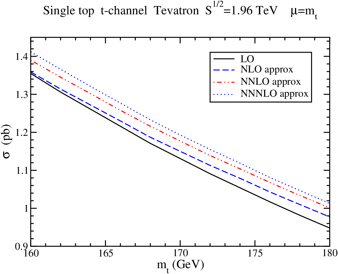

Figure 3 shows the results for the cross section in the channel. On the left we show the LO cross section as well as the cross sections with the NLO, NNLO, and NNNLO soft-gluon corrections included versus the top quark mass , with the factorization and renormalization scales set equal to . On the right we plot the scale dependence of the cross section with GeV. Here we set the factorization scale equal to the renormalization scale and vary this scale over a large range.
We continue with the channel. The soft-gluon corrections approximate the full QCD corrections very well. The corrections are relatively large for this channel, in stark contrast with the results we found in the channel. The matched cross section (exact NLO + soft gluon corrections through NNNLO) is
while for GeV it is pb.
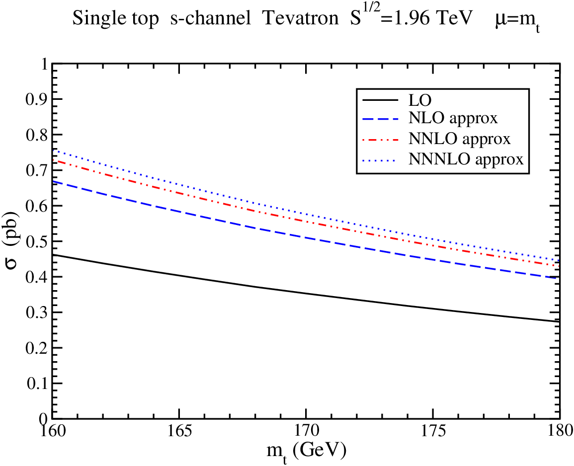
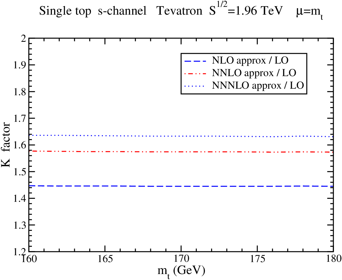
In Fig. 4 we plot the cross section for single top quark production at the Tevatron in the channel as a function of setting the scales to . On the left we plot the LO cross section and the approximate NLO, NNLO, and NNNLO cross sections at NLL accuracy. The factors are quite large and are shown on the right.
The cross section for single top production at the Tevatron via the channel is numerically the smallest. The approximate NNNLO cross section is
and it is pb for GeV.
3.2 Single top production at the LHC
We now show results for single top production at the LHC with TeV. At the LHC the top and antitop cross sections are different in the and channels.
In the channel the threshold corrections are not a good approximation of the full QCD corrections. The exact NLO cross section is pb for GeV, and pb for GeV. For antitop production in the channel the exact NLO cross section is pb for GeV, and pb for GeV.
For single top production at the LHC through the channel the matched cross section, i.e. exact NLO plus soft gluon corrections through NNNLO, is
and the corresponding cross section for GeV is pb.
For single antitop production at the LHC in the channel the matched cross section is
and it is pb for GeV.


In Fig. 5 we plot the cross section for single top quark (left) and single antitop quark (right) production at the LHC in the channel as a function of setting the scales to .
For the channel, the matched cross section (exact NLO [19] plus NNNLO soft corrections) is
and the result for GeV is pb. The cross section for anti-top production in this channel is identical to that for top.


In Fig. 6 we plot the cross section (left) and factors (right) for production at the LHC as functions of , setting the scales to . The higher-order corrections are quite significant as shown by the large factors.
4 Higgs production via
The process has a very simple color structure and kinematics, and is very similar to the Drell-Yan process. The QCD corrections are fully known to NNLO [20]. We can can calculate all soft corrections fully to NNNLO [13, 14]. However, it is found that the soft-gluon approximation is inadequate: purely collinear terms must be included to provide a good approximation. The collinear terms can be resummed at LL accuracy, and good approximations at NLL and NNLL accuracy were provided in [14]. Below we provide numerical results for the cross section at the Tevatron and the LHC using the MRST 2006 parton densities [21].


In Fig. 7 we show the contribution of various terms to the complete NNLO corrections for Higgs production via with at the Tevatron (left-hand side) and the LHC (right-hand side). In this figure NNLO denotes the corrections only, without the LO term and NLO corrections. The curve marked NNLO S+V / NNLO denotes the percentage contribution of the NNLO soft plus virtual (S+V) corrections to the total NNLO corrections. We see that both at the Tevatron and the LHC this contribution is small. Inclusion of the leading collinear (LC) logarithms accounts for about 60% of the total NNLO corrections at both the Tevatron and the LHC. Including the next-to-leading collinear (NLC) logarithms vastly improves the approximation. The difference between the S+V+LC and the S+V+NLC curves is around 30% at the Tevatron and 40% at the LHC; thus the NLC terms are of great importance in achieving a good approximation. We also plot a curve (S+V+NNLC) that in addition includes the next-to-next-to-leading collinear (NNLC) terms. The NNLC terms alone do not make a large contribution, and the S+V+NNLC results approximate the exact NNLO corrections very well, especially at the LHC.
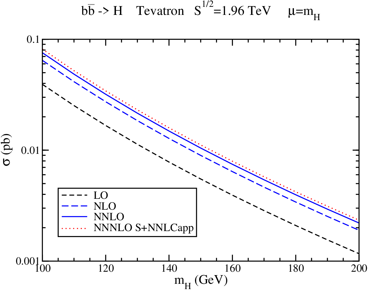
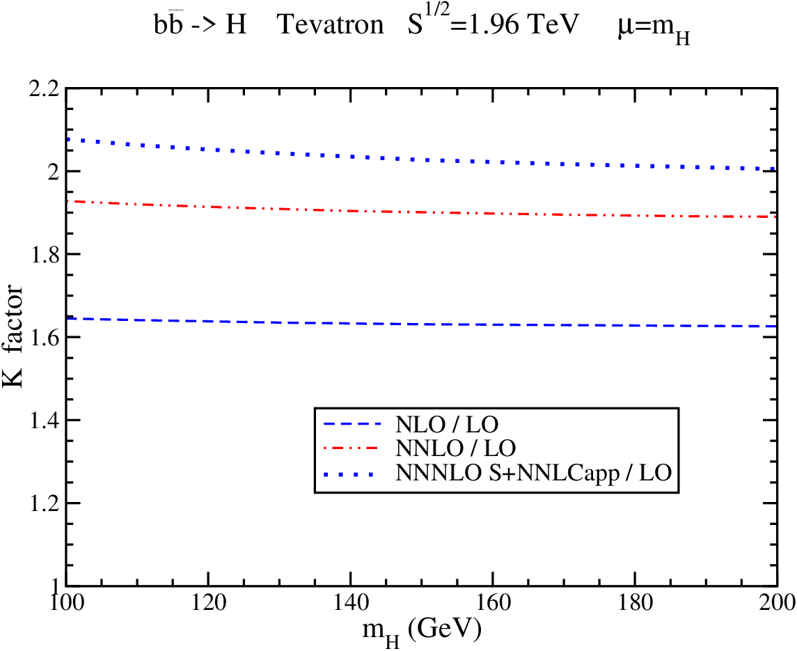
In Fig. 8 we plot the cross sections (left) and factors (right) for at the Tevatron with . The complete NLO corrections increase the LO result by over 60%. The NNLO corrections futher increase the cross section by roughly an additional 30%. Finally, we include the soft and purely collinear corrections at NNNLO. The soft corrections are complete and the purely collinear terms are approximate. Our study of the contributions of the soft and collinear terms at NNLO gives us confidence that the NNNLO S+NNLCapp curves provide a good approximation of the complete NNNLO cross section. The NNNLO S+NNLCapp corrections provide an additional 10% to 15% increase to the cross section.
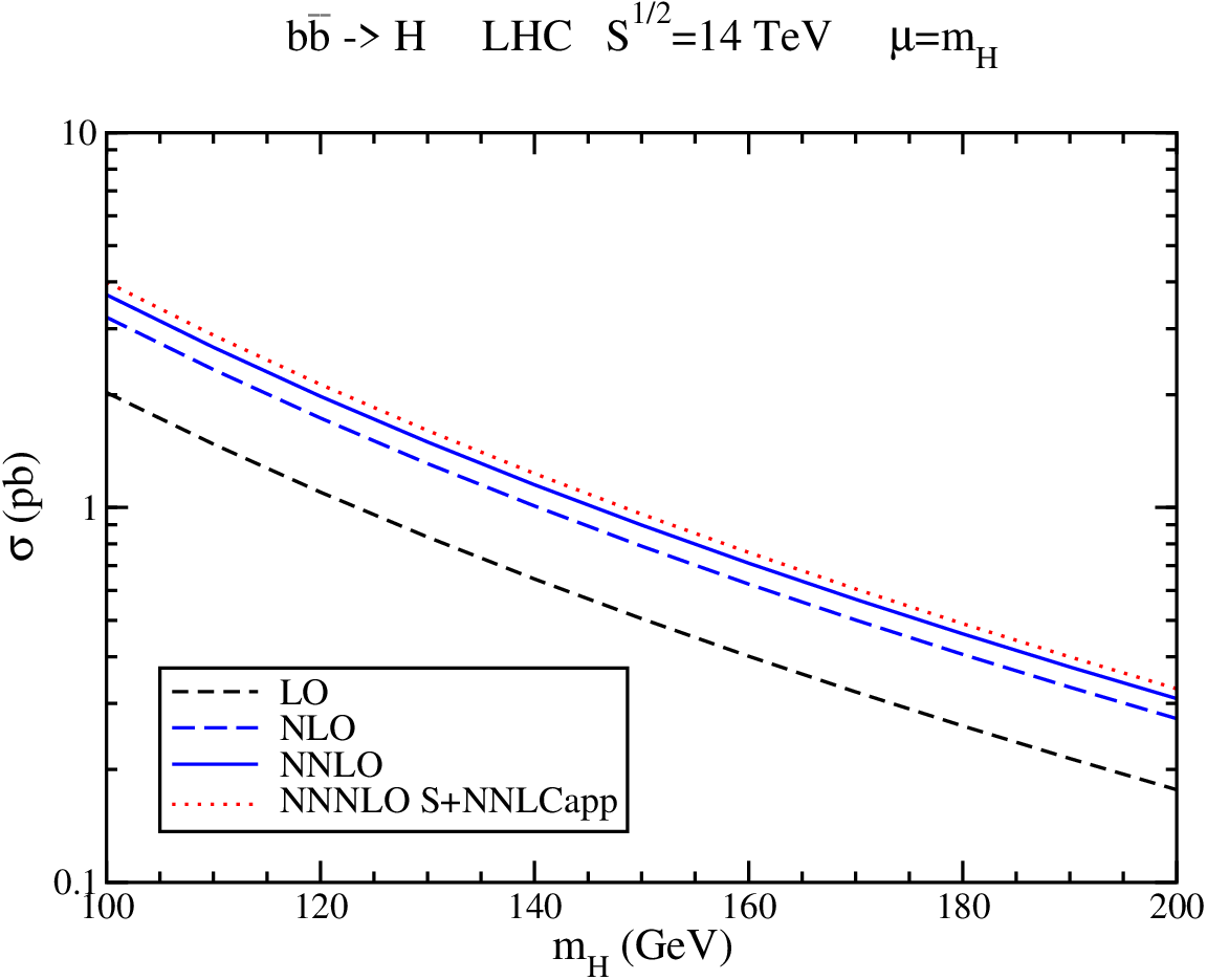
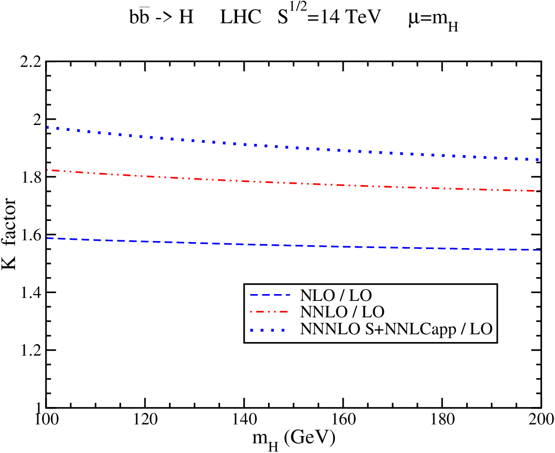
In Fig. 9 we plot the cross sections (left) and factors (right) for at the LHC for . We see that the factors here are quite similar (slightly smaller) to those for the Tevatron.
Finally, we note that the parton distribution function uncertainties for this process are non-negligible and can be of the same order of magnitude as the scale uncertainty, especially for large Higgs masses at the Tevatron.
5 Conclusion
The soft and collinear corrections make important contributions in the cross sections for single top quark production and for Higgs boson production at the Tevatron and the LHC. From the resummation formalism we have derived NNNLO expansions which we use to calculate these corrections.
For single top quark production the soft approximation works well for all channels at the Tevatron, and for the channel and production at the LHC. The soft-gluon corrections are quite significant.
For Higgs production via the process we also have to include purely collinear terms. The collinear+soft approximation is excellent and the corrections through NNNLO are considerable.
Acknowledgements
This work was supported by the National Science Foundation under Grant No. PHY 0555372.
References
- [1] CDF Collaboration, Phys. Rev. Lett. 74, 2626 (1995) [hep-ex/9503002].
- [2] D0 Collaboration, Phys. Rev. Lett. 74, 2632 (1995) [hep-ex/9503003].
- [3] W. Wagner, Rept. Prog. Phys. 68, 2409 (2005) [hep-ph/0507207].
- [4] R. Kehoe, M. Narain, and A. Kumar, Int. J. Mod. Phys. A 23, 353 (2008), arXiv:0712.2733 [hep-ex].
- [5] N. Kidonakis and R. Vogt, Phys. Rev. D 68, 114014 (2003) [hep-ph/0308222].
- [6] CDF Collaboration, Phys. Rev. Lett. 96, 202002 (2006) [hep-ex/0603043]; Phys. Rev. D 74, 072006 (2006) [hep-ex/0607035]; Phys. Rev. D 74, 072005 (2006) [hep-ex/0607095]; Phys. Rev. D 76, 072009 (2007), arXiv:0706.3790 [hep-ex].
- [7] D0 Collaboration, Phys. Rev. D 74, 112004 (2006) [hep-ex/0611002]; Phys. Rev. D 76, 072007 (2007) [hep-ex/0612040]; Phys. Rev. D 76, 092007 (2007), arXiv:0705.2788 [hep-ex]; Phys. Rev. D 76, 052006 (2007), arXiv:0706.0458 [hep-ex].
- [8] D0 Collaboration, Phys. Rev. Lett. 98, 181802 (2007) [hep-ex/0612052].
- [9] CDF Collaboration, Conf. Note 8964; Conf. Note 8968.
- [10] P.W. Higgs, Phys. Rev. Lett 12, 132 (1964); Phys. Rev. Lett. 13, 508 (1964); Phys. Rev. 145, 1156 (1966); F. Englert and R. Brout, Phys. Rev. Lett. 13, 321 (1964); G.S. Guralnik, C.R. Hagen, and T.W.B. Kibble, Phys. Rev. Lett. 13, 585 (1964).
- [11] The Higgs Working Group: Summary Report, in Les Houches 2003, Physics at TeV colliders, p. 1 [hep-ph/0406152], and references therein.
- [12] N. Kidonakis, Phys. Rev. D 74, 114012 (2006) [hep-ph/0609287]; Phys. Rev. D 75, 071501(R) (2007) [hep-ph/0701080]; in DIS2007, p.443, arXiv:0705.2431 [hep-ph].
- [13] V. Ravindran, Nucl. Phys. B 752, 173 (2006) [hep-ph/0603041].
- [14] N. Kidonakis, Phys. Rev. D (in press), arXiv:0711.0142 [hep-ph].
- [15] N. Kidonakis, Int. J. Mod. Phys. A 19, 1793 (2004) [hep-ph/0303186]; Mod. Phys. Lett. A 19, 405 (2004) [hep-ph/0401147]; in DIS2003, p. 429, hep-ph/0307207; in DIS2003, p. 465, hep-ph/0306125; in DPF2004, Int. J. Mod. Phys. A 20, 3726 (2005) [hep-ph/0410116].
- [16] N. Kidonakis, Phys. Rev. D 73, 034001 (2006) [hep-ph/0509079]; PoS (HEP2005) 055 (2006) [hep-ph/0512017]; in DIS 2006, p. 463, hep-ph/0606280.
- [17] A.D. Martin, R.G. Roberts, W.J. Stirling, and R.S. Thorne, Phys. Lett. B 604, 61 (2004) [hep-ph/0410230].
- [18] B.W. Harris, E. Laenen, L. Phaf, Z. Sullivan, and S. Weinzierl, Phys. Rev. D 66, 054024 (2002) [hep-ph/0207055].
- [19] S.H. Zhu, Phys. Lett. B 524, 283 (2002) [hep-ph/0109269]; (E) B 537, 351 (2002).
- [20] R.V. Harlander and W.B. Kilgore, Phys. Rev. D 68, 013001 (2003) [hep-ph/0304035].
- [21] A.D. Martin, W.J. Stirling, R.S. Thorne, and G. Watt, Phys. Lett. B 652, 292 (2007) [arXiv:0706.0459].