Analysis of the exciton-exciton interaction in semiconductor quantum wells
Abstract
The exciton-exciton interaction is investigated for quasi- two-dimensional quantum structures. A bosonization scheme is applied including the full spin structure. For generating the effective interaction potentials, the Hartree-Fock and Heitler-London approaches are improved by a full two-exciton calculation which includes the van der Waals effect. With these potentials the biexciton formation in bilayer systems is investigated. For coupled quantum wells the two-body scattering matrix is calculated and employed to give a modified relation between exciton density and blueshift. Such a relation is of central importance for gauging exciton densities in experiments which pave the way toward Bose-Einstein condensation of excitons.
pacs
73.20.Mf, 71.35.Gg, 78.67.DeI Introduction
Excitons (bound pairs of electron and hole) play a key role in semiconductor optics, and their theoretical understanding has a long history.[1] Although excitons obey Bose statistics, the fermionic structure of their constituents is always important and forbids to treat excitons as nearly ideal Bose particles. Among the first attempts for bosonization of excitons, we quote Refs. 2, 3, 4. Both the fermionic exchange and the Coulomb forces between two excitons can be condensed into an effective exciton-exciton (XX) interaction potential. Efforts for deriving XX potentials are abound in the literature, covering three-dimensional excitons in bulk semiconductors as well as quasi-two-dimensional excitons in quantum wells. However, almost all of these attempts[5, 6, 7, 8] were restricted to the Hartree-Fock level, i.e., taking into account the XX interactions up to second order in the elementary charge, . Sometimes it has been claimed that this would be enough for treating sufficiently accurate the exciton gas at low density . This is not correct since already at zero density, the single-exciton bound state calls for an infinite summation in powers of the Coulomb potential, and consequently the next term (linear in ) cannot be truncated either. It was not before 2001 that in a seminal paper by Okumura and Ogawa[9] the first XX potential beyond Hartree-Fock[10] for bulk semiconductors has been constructed, in close analogy to the Heitler-London approximation in atomic physics.
The interest in a proper description of XX interactions has been surely intensified by the actual search for Bose-Einstein condensation of excitons, which has been predicted theoretically already decades ago.[11, 13, 12] Due to the small exciton mass compared to atomic systems, the critical temperature for the condensate is expected to be a few kelvins for a density of in bulk GaAs, within easy reach experimentally. A fundamental problem, however, is the finite life time of the excitons, which hinders the relaxation into thermal equilibrium. One possible way out are coupled quantum wells (CQWs) which came into focus a few years ago.[14, 15, 16, 17, 18] A static electric field in growth direction forces electrons and holes to reside in adjacent quantum wells which are separated by a barrier. Due to this spatial separation, the indirect excitons exhibit extremely long life times, which is a good condition for reaching thermal equilibrium. However, these spatially indirect excitons form dipoles leading to a strong and long-range repulsion, which complicates the theoretical description as well as the experimental realization of a dense cold exciton gas. [19, 20] Recently large progress has been reported for spatially indirect excitons in electrostatic[21] as well as optical traps. [22, 23]
These practical demands led us to investigate the XX interaction in more detail, with special emphasis on coupled quantum wells. In particular, we improve on the Heitler-London-type treatment in Ref. 9 by solving the four-particle Schrödinger equation for two electrons and two holes numerically. Before doing so we address the complex spin structure of the exciton composed of a spin 1/2 electron and a spin 3/2 heavy hole (Sec. II). The importance of spin-dependent effects in the exciton gas has been emphasized e.g., in Ref. 24. In the limit of immobile holes (their mass being usually much larger than that of the electrons), we can derive effective spin-dependent XX potentials (Sec. III) which contain in addition to the dipole-dipole repulsion and exchange effects the weak van der Waals forces. The latter is of importance to rectify a recent claim[25, 26] to have explained the bead pattern formation which appears at low temperatures in the ring-shaped CQW emission.[27, 28, 29]
With a proper XX interaction at hand, we are able to calculate biexciton states (excitonic molecules), which are well known from bulk semiconductors and have been observed in single quantum wells.[30, 31] Since biexciton energies have been calculated with high precision elsewhere,[32] we use these results to judge our approximate treatment in Sec. IV. For the CQW situation simplified to a bilayer system, we identify the parameter values (essentially mass ratio and charge separation) which limit the existence of biexcitons.
Addressing the many-exciton case, we will treat the excitons as effective bosons with a renormalized interaction potential, derived from the underlying electron-hole description. [33] As an application, we investigate in Sec. V two realistic CQW structures. The numerically generated XX potentials are used to calculate two-exciton scattering phase shifts which are the main ingredient for a -matrix based quasi-particle dispersion[34]. For the low-density case, we are able to calculate excitonic blueshift and scattering-induced broadening linear in (Sec. VI). We find a stunning reduction of the blueshift compared to the simple ”capacitor formula” and relate this finding to features in the XX pair-correlation function which - due to the strong repulsion - resembles more a Fermi gas than a free Bose gas (Sec. VII).
Conclusions are drawn in Sec. VIII, while a few technical details are deferred to the Appendix.
II Many-Exciton Hamiltonian
To derive the many-exciton Hamiltonian we follow the work of de-Leon and Laikhtman.[8, 35] The task is to find the matrix elements of the electron-hole Hamiltonian with an appropriate two-exciton wave function and to implement them into an effective bosonic Hamiltonian for many excitons. The effective-mass Hamiltonian for two electrons and holes reads
| (1) |
where the interaction part [second and third line of Eq. (1)] is composed of Coulomb interactions between particle and , which can be either electron () or hole (),
| (2) |
Please note that the corresponding sign (attractive or repulsive) has been made explicit in Eq. (1).
We define exciton quantum field operators which create an exciton at exciton center-of-mass (c.m.) position with spin , and , which annihilates the same exciton. The subsequent Hamilton operator will be written as
| (3) |
with the exciton mass in the kinetic energy. is the spin and space-dependent pair interaction potential. In the following, it will be extracted from a careful study of the four-particle problem [Eq. (1)]. The exciton spin index is the sum of the electron spin () and the heavy-hole angular momentum (). We neglect the light holes, which are separated due to the confinement effects in the quasi-two-dimensional quantum well (QW). Now, runs over four values (bright states) and (dark states). Since electron and hole are fermions, we have to use a properly symmetrized ansatz for both component’s spin wave functions and , which make the overall wave- function antisymmetric with respect to the exchange of the electrons and the holes, respectively. The labels and denote the parity which can be symmetric or antisymmetric . Together with the spatial part we write the total two-exciton wave function,
| (4) |
where the upper label stands for the electron part, and the lower one for the hole part. Please note that due to the fermionic nature of the particles, the parities of the spin part and of the spatial part have to be opposite to each other. Taking now the matrix elements of Eq. (1) with the ground state wave functions we get four different potentials,[36]
| (5) |
Due to the one to one correspondence between the exciton spin and the spin of its constituents, it is possible to express the basis vectors in the space of symmetric and antisymmetric spin wave functions by the spin eigenstates of the excitons . After a straightforward unitary transformation one gets the interaction matrix elements as shown in Table 1 for columns and rows . Here and similar for the lower hole index.
![[Uncaptioned image]](0802.3337v2/tbl1_W_spin_struct.png)
![[Uncaptioned image]](0802.3337v2/tbl2_W_0_spin_struct.png)
We can clearly see the block structure of the interaction which reflects the conservation of the total spin . The interaction channels can be classified as follows: There is the direct channel where an initial state will remain unchanged. The other channel is of exchange type with a change in the initial state due to three different processes: Exchange of electrons, exchange of holes, and exchange of both simultaneously. The electron-hole exchange process (longitudinal-transverse splitting of the exciton) has been neglected already in the starting Hamiltonian.
In a case where the hole mass is much larger than the electron mass, the exchange of holes becomes negligible and the four different potentials [Eq. (5)] collapse into two, and , which correspond to wave functions properly symmetrized only with respect to the electrons. In this case the interaction part of the Hamiltonian simplifies to the form shown in Table 2 where and can be cast into the form given in the Appendix, [Eq. (24)].
III Effective interaction potentials
To derive the spatial dependence of the interaction potentials introduced in Sec. II, approximations have been introduced in the literature. In the infinitely heavy-hole limit, the Heitler-London ansatz is well known from atomic physics and has recently been brought into exciton physics by Okumura and Ogawa.[9] In a bulk semiconductor, the two excitons resemble a hydrogen molecule in this limit. The problem of four particles (two electrons and two holes) simplifies here to a two-particle problem for the electrons, while the hole-hole distance enters as a parameter. Therefore, the Coulomb potential between the holes gives just a fixed additional term in the Hamiltonian. The two-exciton wave function can then be written as a properly antisymmetrized product of single-exciton wave functions in the ground state , centered around the position of each hole. For the spatial part of the two-exciton wave function, we can write
| (6) |
with the wave function overlap,
| (7) |
which leads to the potentials,
| (8) |
with direct and exchange potential [explicit expressions are given in the Appendix, Eq. (27) and Eq. (28)].
A simplified version of the Heitler-London approximation, which has usually been applied to excitonic systems,[5, 37, 6, 8] is the famous Hartree-Fock treatment where the normalization denominator in Eq. (6) is left out and is consequently missing in Eq. (8). This scheme can easily be generalized to arbitrary hole masses. However, it leads to a nonlocal exchange potential[5] and to problems with the orthogonality of the basis states.[38]
To improve over the approximations discussed so far, we have solved the Schrödinger equation for the two electrons numerically using the Lanczos algorithm, treating the holes as infinitely heavy and thus immobile. The equation to be solved reads
| (9) |
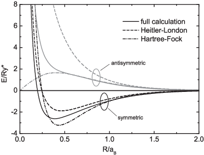
where is the effective electron mass in the plane and is the single-exciton binding energy. The zero of energy is chosen to be the band gap. Fig. 1 shows the resulting effective interaction potentials in Hartree-Fock, Heitler-London, and full numerical quality exemplarily for a strictly two-dimensional system. We note the unphysical behavior of the Hartree-Fock antisymmetric potential which approaches zero for small distances. It also misses the proper sequence of the antisymmetric channel to be above the symmetric one for small distances. This is the result of leaving out the normalization denominator in Eq. (6). Thus these problems are corrected in the Heitler-London treatment. Here also the antisymmetric channel shows the expected Coulomb singularity of the hole-hole potential for small distances. In the full solution the energy is lowered compared to the Heitler-London approximation by a mutual deformation of the excitonic orbitals. Please note that the van der Waals effect is included due to the nonperturbative nature of the calculation.
While the considerations above are correct also in three dimensions, we turn now to the two-dimensional case of quantum structures. All vectors are to be understood as lying in the x-y plane, the z-axis being the growth direction.
We note that all interaction potentials in Fig. 1 approach zero from positive values and hence show a repulsion for larger distances, although this is hardly seen in Fig. 1. However, this behavior follows already from a multipole expansion of the direct potential , which dominates the interaction at large distances. In such an approach we treat the exciton as a static charge distribution with cylindrical symmetry and centered at zero c.m. coordinate. The specific form of depends on the system under investigation and will be specified later. Due to the charge neutrality of the exciton the multipole expansion starts with the dipole term , where denotes the in plane c.m. distance of the two excitons. Up to the quadrupole term we obtain for the asymptotics
| (10) |
where the angular brackets denote averaging over . For a bulk system with spherical symmetry we see immediately that the multipole expansion vanishes as expected. However, for the reduced symmetry of quasi-two-dimensional systems, we get finite multipoles also for in-plane circular symmetry. Even for the strictly two-dimensional system, where , there is a contribution from the quadrupole-quadrupole interaction (). This holds as well for symmetric single QWs where due to the mirror symmetry along the z-axis. The direct interaction thus falls off as a power law rather than exponentially, which has been overlooked in a recent investigation of the asymptotic XX potential.[25] In Fig. 2 we compare the asymptotic behavior of the numerically calculated direct potential [Eq. (27)], and the result from the multipole expansion [Eq. (10)] using the strictly two-dimensional charge distribution for an immobile hole and the usual Coulomb potentials [Eq. (2)]. The multipole expansion holds for . The full solution shows the van der Waals effect and lies below the direct potential. However, this effect is not able to overcome the repulsive nature of the asymptotic potential.

To grasp this effect a bit more quantitatively, we plot in Fig. 3 the difference between the direct potential from the approximations of rigid orbitals and a corresponding quantity for the full solution (). For very large distances , we fit this difference to a van der Waals potential, i.e., a power law (dashed line in Fig. 3). The van der Waals law holds only for distances .

For smaller distances higher-order effects come in and spoil the dependence.
With the derived effective interaction potentials, we construct the two-dimensional Schrödinger equation for two excitons with mutual distance in c.m. space, where we introduce now the finite exciton mass in the kinetic term:
| (11) |
where denotes the angular quantum number. Please note the missing factor of 2 in the denominator of the kinetic term since we have to consider the reduced mass of two excitons, .
IV Model Systems
To test the reliability of our Born-Oppenheimer-type method, we calculate the biexciton binding energy from the lowest state of Eq. (11) with for different mass ratios in the strictly two-dimensional limit. These results are compared in Fig. 4 with variational calculations from the literature[32] which are numerically exact. As expected, our method produces exact results for . For nonzero mass ratio we underestimate the binding energy slightly, e.g., for we have an error of . Even for the error is only about . We conclude that the method is a reasonable approximation for GaAs quantum structures (), which will be under investigation in Sec. V.

We plot the Haynes factor for the other approximations as well (for the strictly two-dimensional system, ). The Heitler-London approximation underestimates the biexciton binding energy significantly. Hartree-Fock seems to do much better, but note that for small the Haynes factor is overestimated, which is in contrast to the variational principle.
A simple model for a coupled quantum well structure is the so- called bilayer system:[39] Electrons and holes are confined each in infinitely narrow planes with a separation between the layers. This separation of unequal charges leads to a reduced Coulomb interaction between particles in different layers but leaves the potentials between particles of the same kind unchanged,
| (12) |
The charge distribution reads now , and the expansion [Eq. (10)] yields a finite dipole-dipole interaction , resulting in a strong long-range repulsion. For the many-exciton problem we are in particular interested in the biexciton formation. Fig. 5 shows the biexciton binding energy versus charge separation for a mass ratio of and . In both cases we find a fast reduction of with increasing separation between the layers as expected. At a certain critical charge separation , denoted by arrows in Fig. 5, the biexciton ceases to exist. The same model system has been investigated by Tan et al.[39] using quantum Monte Carlo (QMC) technique. From their results at intermediate values of , which agree nicely with our own calculations, the authors suggested an exponential decay of for large . The inset of Fig. 5 shows the potential in the symmetric channel for different values of the charge separation. It is clearly seen how the potential minimum passes through zero with increasing and vanishes completely if is enlarged further (large arrow). Therefore a (finite) critical charge separation exists where the biexciton binding energy becomes zero due to the dominant dipole-dipole repulsion. More recently this critical behavior was also observed in QMC calculations of Lee and Needs.[40]

In Fig. 6 we plot the critical charge separation vs mass ratio. Below this curve, in the shaded area, bound states can be formed, while above no biexcitons exist. For small we obtain a rapid decrease of the critical charge separation. For larger mass ratios, on the other hand, the separation does not depend much on . This behavior resembles Fig. 4, revealing a direct connection between biexciton binding energy and critical charge separation.

V Results for Coupled Quantum Wells
We turn now to realistic coupled quantum well structures, having GaAs as well material and barriers made of . In this case we treat the Coulomb interaction in single sublevel approximation,[41, 33] which is given by
| (13) |
Here, is again an in-plane vector, and and denote the confinement functions of the lowest sublevel for electron and hole. They enter as well the static charge distribution of the exciton: . Fig. 7 shows the effective interaction potentials for a GaAs/ coupled quantum well geometry used by Butov[28] with a nominal (i.e., center distance between the wells) charge separation of (sample A in Table 3). We see again the already discussed features of the three approximation levels. The energy gain when going from Heitler-London to the full calculation yields a minimum for the symmetric channel, which however is so weak that no biexcitons can be formed. This feature strongly depends on the geometry of the quantum wells, which is illustrated in Fig. 8. Here the full calculation potentials for sample A are compared to another one used by Snoke et al.[42] where (sample B in Table 3). Due to the larger charge separation no minimum can be seen in the symmetric channel. This observation is consistent with the results obtained for the idealized (bilayer) model discussed in Sec. IV.
| Sample A | Sample B | |
| Well width (nm) | ||
| Barrier width (nm) | ||
| (nm) | ||
| (nm) | ||
| Static field (kV/cm) | 30.0 | 36.0 |
| (meV) |
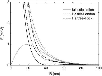
With these results a simple explanation for the regular bead pattern in the luminescence ring at low temperatures[27, 28, 29] has to be ruled out: It was speculated[25, 26] that the van der Waals effect could overcome the dipole-dipole repulsion, resulting in an attraction between spatially indirect excitons, which would lead to a spontaneous patterning. Our calculation shows that this is not the case in agreement with recent experimental investigations. [43, 44] In Ref. 25 the quadrupole-quadrupole interaction in two-dimensional systems has been overlooked and hence the role of the van der Waals force overestimated as discussed in Sec. IV.

VI Exciton Blueshift and Broadening
We turn now to the calculation of the interaction induced blueshift and broadening which can be observed in photoluminescence experiments.[42, 45, 46] In a point charge treatment of spatially indirect excitons, we have from Eq. (27)
| (14) |
Plugging in Eq. (12) for the bilayer system, one gets a dipole-dipole repulsion of the form
| (15) |
Assuming a homogeneous exciton density , this leads to a blueshift,
| (16) |
Since this expression is consistent with the electrostatics of a plate capacitor, it is often referred to as capacitor formula.[47] We will derive a corrected formula for the blueshift and the scattering-induced broadening using the effective interaction potentials given in Fig. 8. The exciton self energy is calculated in a -matrix approach.[34] In the low-density limit and assuming complete spin equilibrium, we write the two-body -matrix equation as
| (17) |
The -matrix enters the quasiparticle self-energy as boson-direct (D) and boson-exchange (X),
| (18) |
where is put on shell and is the exciton

distribution function, which is later taken as the low-density Maxwell-Boltzmann expression. The spin structure of the Hamiltonian yields the following decomposition in the limit of immobile holes:
| (19) |
The on-shell -matrix needed in Eq. (18) depends exclusively on the phase shifts via[48]
| (20) |
We have extracted the phase shifts from the asymptotics of the solution of the radial Schrödinger equation [Eq. (11)] for . Results for the total complex scattering amplitude [curly bracket in Eq. (18)] are shown in Fig. 9. Please note that for large momenta , the real part of the scattering amplitude approaches the prediction of the capacitor formula but with an effective charge separation which is somewhat below the nominal one (third and forth row of Table 3). This reduction is due to the spatial extension of electron and hole charges along . A simple argument assuming confinement wave functions for infinite barriers leads to . This is quite close to the numerical value which follows from replacing the point charge potential [Eq. (15)] in Eq. (16) by the numerically derived one.
Using the scattering amplitude, we calculate the quasiparticle shift and broadening at the dispersion edge () and introduce correction factors , to the capacitor formula
| (21) |
The real part of this quantity is the blueshift of the exciton due to the repulsive interaction, while the imaginary part can be associated with a finite broadening. Please note that with the sign convention used, is negative. The correction factors shown in Fig. 10 reduce the capacitor result dramatically. Therefore, the density for a measured blueshift would be underestimated by a factor of 10 at low temperatures. The broadening is of the same order of magnitude, which is consistent with experimental findings.

VII Exciton-Exciton correlation function
The significant reduction of the quasiparticle shift compared to the capacitor value can be explained with a strong depletion of the exciton gas around a given exciton due to the repulsive interaction. To grasp this repulsive correlation more directly we calculate the exciton pair- correlation function:
| (22) |
It has the same spin structure as the -matrix. In the spin equilibrated situation investigated here, the exciton density does not depend on spin. Summing over both spin indices, we obtain with a partial wave decomposition,
| (23) |
The results shown in Fig. 11 reflect the strong repulsion of the excitons independent of the spin channel. It is interesting to compare with the pair-correlation function of ideal bosons and fermions having four spin degrees of freedom as well. Obviously in the present case, the repulsive interaction between excitons is much more important than the bosonic nature of their statistics.

VIII Conclusions
In the investigation of the many-exciton problem in semiconductor quantum structures, we have found a much richer spin structure with spatially dependent interaction potentials than with just contact interactions. This is due to non trivial exchange processes of the fermionic constituents. For the spatially dependence of the potentials, we compared three different levels of approximation: The Hartree-Fock and the Heitler-London approximations as well as a newly introduced full numerical solution of the two exciton problem. We found a principal failure of the Hartree-Fock treatment, which is cured in the Heitler-London approach. The quality of the latter, however, turns out to be quite poor, compared to numerically exact results. With our calculated potentials we have investigated bilayer systems and two different CQWs. The charge separation plays a fundamental role: By tuning a transition happens from systems with possible biexciton formation to those where biexcitons are not bound due to the stronger XX repulsion. For two realistic CQW structures we have calculated the quasiparticle shift and broadening at the band edge which govern roughly the photoluminescence line shape. At low temperatures, we found a dramatic reduction of the blueshift compared to a naive treatment of the CQW as plate capacitor. The broadening turns out to be of the same order as the blueshift.
Acknowledgements.
Numerous stimulating discussions with Leonid Butov, Boris Laikhtman, Vincenzo Savona, and Dave Snoke are gratefully acknowledged.Appendix A
In the limit of infinitely heavy holes, the interaction part of the many-exciton Hamiltonian (Table 2) can be written as[33]
| (24) |
For the simplifications of contact potentials , our result agrees with the one derived by de-Leon and Laikhtman.[8] This can be seen as follows: Plugging the contact potentials into Eq. (24) the integration over can be carried out immediately,
| (25) |
In this limit, the third row of Eq. (24) gives no contribution. We can also drop the Heaviside step function by inserting a factor of to account for the double counting in the sum over and and get
| (26) |
In the language of the Hartree-Fock approximation, we can trade the symmetric and the antisymmetric potentials for the direct and the exchange ones. For arbitrary hole masses, and have been derived in the literature.[6] For immobile holes they reduce to the direct potential,
| (27) |
and the exchange potential,
| (28) |
Taken in the contact limit and , Eq. (26) can be written as
| (29) |
The Fourier transform of this result yields the Hamiltonian
derived in Ref. 8.
References
- [1] R. Knox, Theory of Excitons, Solid State Physics Suppl. 5 (Academic, New York, 1963).
- [2] T. Usui, Progr. Theor. Phys. 23, 787 (1960).
- [3] L. V. Keldysh and A. N. Kozlov, Sov. Phys. JETP 27, 521 (1968).
- [4] E. Hanamura and H. Haug, Phys. Rep. 33, 209 (1977).
- [5] C. Ciuti, V. Savona, C. Piermarocchi, A. Quattropani, and P. Schwendimann, Phys. Rev. B 58, 7926 (1998).
- [6] J.-i. Inoue, T. Brandes, and A. Shimizu, Phys. Rev. B 61, 2863 (2000).
- [7] G. Rochat, C. Ciuti, V. Savona, C. Piermarocchi, A. Quattropani, and P. Schwendimann, Phys. Rev. B 61, 13856 (2000).
- [8] S. Ben-Tabou de-Leon and B. Laikhtman, Phys. Rev. B 63, 125306 (2001).
- [9] S. Okumura and T. Ogawa, Phys. Rev. B 65, 035105 (2001).
- [10] An early attemp including some features of the Heitler-London method to excitons is found in: A. I. Bobrysheva, phys. stat. sol. 16, 337 (1966).
- [11] S. A. Moskalenko, Sov. Phys.-Solid State 4, 199 (1962), (Engl. Transl.).
- [12] Y. E. Lozovik and V. I. Yudson, JETP Lett. 22, 274 (1975).
- [13] L. V. Keldysh and Y. V. Kopaev, Sov. Phys.-Solid State 6, 2219 (1965), (Engl. Transl.).
- [14] L. V. Butov, A. Zrenner, G. Abstreiter, G. Böhm, and G. Weimann, Phys. Rev. Lett. 73, 304 (1994).
- [15] V. B. Timofeev, A. V. Larionov, M. Grassi-Alessi, M. Capizzi, and J. M. Hvam, Phys. Rev. B 61, 8420 (2000).
- [16] L. V. Butov, C. W. Lai, A. L. Ivanov, A. C. Gossard, and D. S. Chemla, Nature 417, 47 (2002a).
- [17] D. Snoke, S. Denev, Y. Liu, L. Pfeiffer, and K. West, Nature 418, 754 (2002).
- [18] D. Snoke, Science 298, 1368 (2002).
- [19] R. Rapaport, G. Chen, and S. H. Simon, Phys. Rev. B 73, 033319 (2006).
- [20] G. Chen, R. Rapaport, L. N. Pffeifer, K. West, P. M. Platzman, S. Simon, Z. Voros, and D. Snoke, Phys. Rev. B 74, 045309 (2006).
- [21] Z. Voros, D. W. Snoke, L. Pfeiffer, and K. West, Phys. Rev. Lett. 97, 016803 (2006).
- [22] A. T. Hammack, M. Griswold, L. V. Butov, L. E. Smallwood, A. L. Ivanov, and A. C. Gossard, Phys. Rev. Lett. 96, 227402 (2006).
- [23] A. T. Hammack, L. V. Butov, L. Mouchliadis, A. L. Ivanov, and A. C. Gossard, Phys. Rev. B 76, 193308 (2007).
- [24] G. Aichmayr, M. Jetter, L. Viña, J. Dickerson, F. Camino, and E. E. Mendez, Phys. Rev. Lett. 83, 2433 (1999).
- [25] V. I. Sugakov, Solid State Comm. 134, 63 (2005).
- [26] C. S. Liu, H. G. Luo, and W. C. Wu, J. Phys.: Condens. Matter 18, 9659 (2006).
- [27] L. V. Butov, A. C. Gossard, and D. S. Chemla, Nature 418, 751 (2002b).
- [28] L. V. Butov, Solid State Comm. 127, 89 (2003).
- [29] D. Snoke, Y. Liu, S. Denev, L. Pfeiffer, and K. West, Solid State Comm. 127, 187 (2003).
- [30] D. A. Kleinman, Phys. Rev. B 28, 871 (1983).
- [31] R. C. Miller, D. A. Kleinman, A. C. Gossard, and O. Munteanu, Phys. Rev. B 25, 6545 (1982).
- [32] J. Usukura, Y. Suzuki, and K. Varga, Phys. Rev. B 59, 5652 (1999).
- [33] R. Zimmermann and C. Schindler, Solid State Comm. 144, 395 (2007).
- [34] R. Zimmermann, phys. stat. sol. (b) 243, 2358 (2006).
- [35] S. Ben-Tabou de-Leon and B. Laikhtman, Europhys. Lett. 59, 728 (2002).
- [36] J. J. Forney, A. Quattropani, and F. Bassani, Il Nuovo Cimento 22, 153 (1974).
- [37] R. Zimmermann, Solid State Comm. 134, 43 (2005).
- [38] B. Laikhtman, J. Phys.: Condens. Matter 19, 295214 (2007).
- [39] M. Y. J. Tan, N. D. Drummond, and R. J. Needs, Phys. Rev. B 71, 033303 (2005).
- [40] R. M. Lee and R. Needs (2008), private communication.
- [41] S. de-Leon and B. Laikhtman, Phys. Rev. B 61, 2874 (2000).
- [42] D. W. Snoke, Y. Liu, Z. Vörös, L. Pfeiffer, and K. West, Solid State Comm. 134, 37 (2005).
- [43] R. Rapaport, G. Chen, D. Snoke, S. H. Simon, L. Pfeiffer, K. West, Y. Liu, and S. Denev, Phys. Rev. Lett. 92, 117405 (2004).
- [44] S. Yang, A. V. Mintsev, A. T. Hammack, L. V. Butov, and A. C. Gossard, Phys. Rev. B 75, 033311 (2007).
- [45] L. V. Butov, A. Imamoglu, A. A. Shashkin, V. T. Dolgopolov, A. V. Mintsev, S. Feklisov, K. L. Campman, and A. C. Gossard, phys. stat. sol. (a) 178, 83 (2000).
- [46] V. Negoita, D. W. Snoke, and K. Eberl, Phys. Rev. B 61, 2779 (2000).
- [47] X. Zhu, P. B. Littlewood, M. S. Hybertsen, and T. M. Rice, Phys. Rev. Lett. 74, 1633 (1995).
- [48] S. A. Morgan, M. D. Lee, and K. Burnett, Phys. Rev. A 65, 022706 (2002).