New Physics at a Super Flavor Factory
Abstract
Abstract
The potential of a Super Flavor Factory (SFF) for searches of New Physics is reviewed. While very high luminosity physics is assumed to be at the core of the program, its scope for extensive charm and studies are also emphasized. The possibility to run at the is also very briefly discussed; in principle, this could provide very clean measurements of decays. The strength and reach of a SFF is most notably due to the possibility of examining an impressive array of very clean observables. The angles and the sides of the unitarity triangle can be determined with unprecedented accuracy. These serve as a reference for New Physics (NP) sensitive decays such as and penguin dominated hadronic decay modes, providing tests of generic NP scenarios with an accuracy of a few percent. Besides, very precise studies of direct and time dependent CP asymmetries in radiative decays and forward-backward asymmetry studies in and numerous null tests using , charm and decays are also likely to provide powerful insights into NP. The dramatic increase in luminosity at a SFF will also open up entirely new avenues for probing NP observables, e.g. by allowing sensitive studies using theoretically clean processes such as . The SFF is envisioned to be a crucial tool for essential studies of flavor in the LHC era, and will extend the reach of the LHC in many important ways.
I Introduction
The term flavor was first used in particle physics in the context of the quark model of hadrons. It was coined in 1971 by Murray Gell-Mann and his student at the time, Harald Fritzsch, at a Baskin-Robbins ice-cream store in Pasadena. Just as ice-cream has both color and flavor so do quarks [317].
Flavor physics denotes physics of transitions between the three generations of Standard Model (SM) fermions. With the LHC startup around the corner, why should one pay attention to these low energy phenomena? For one thing, flavor physics can probe new physics (NP) through off-shell corrections, before the NP particles themselves are produced in energy frontier experiments. As a historic example, the existence of the charm quark was predicted from the suppression of before its discovery [339], while its mass was successfully predicted from [321]. Flavor physics is also intimately connected with the origin of fermion masses. In the limit of vanishing masses the flavor physics is trivial – no intergenerational transitions occur since weak and mass eigenbases trivially coincide. It is only the mismatch of weak and mass eigenbases (or the mismatch between the bases in which gauge and Yukawa terms are diagonal) that makes flavor physics interesting. In the quark sector of SM this mismatch is described by a single unitary matrix - the Cabibbo–Kobayashi–Maskawa (CKM) matrix. Finally, CP violation is closely related to flavor physics. A strong argument for the existence of new sources of CP violation is that the CKM mechanism is unable to account for the observed baryon asymmetry of the universe (BAU) through baryogenesis [328]. This points at NP with new sources of CP violation in either the quark or lepton sector (the latter potentially related to the BAU via leptogenesis [578]). It is therefore important to investigate the BAU by studying CP violation in both quark and lepton sectors (see below).
In the past ten years, due to the spectacular performance of the two -factories, a milestone in our understanding of CP violation phenomena was reached. For the first time, detailed experiments, BABAR [72] and Belle [3], provided a striking confirmation of the CKM-paradigm of CP violation [226, 457]. The Kobayashi-Maskawa model of CP-violation, based on three families and a single CP-odd phase, is able to account for the observed CP violation in the system, as well as that in the system, to an accuracy of about 20%, as shown in Fig. 1 [238, 189, 191, 498]. The impressive gain in precision on CKM constraints that is expected at a SFF is also shown in Fig. 1.


While we celebrate this remarkable agreement it is important to note that increasing the accuracy of CKM tests brings more than just an increased knowledge of fundamental CKM parameters. Once NP particles are observed at LHC, flavor physics observables will provide a set of independent constraints on the NP Lagrangian. These constraints are complementary to the measurements that are performed at high processes – i.e. they provide a complementary constraint on the combination of couplings, mixing angles and NP masses and become much more powerful once NP mass spectra are already measured. However, to be relevant for TeV processes, high precision is needed. But, how precise is precise enough? The answer depends on the NP flavor changing couplings. Taking as a conservative benchmark the case of minimally flavor violating NP that has couplings to SM fermions comparable to weak gauge couplings, the present results from factories allow for masses of NP particles below GeV. After completion of the Super Flavor Factory (SFF) program this limit would be pushed to GeV [191, 209], illustrating the complementarity of LHC and SFF reach.11 1 Note that the generic MFV scenario of weakly coupled NP is not the most conservative scenario. The SFF constraint can be avoided, if couplings to SM fermions are further suppressed (see, for instance, Grossman et al. [392].)
Let us elaborate a bit more on this important point. The NP constraints depend on both NP couplings to SM quarks and the NP masses and the two cannot be disentangled. An important set of flavor physics observables useful for NP searches are those from processes that proceed through flavor changing neutral currents. These are loop suppressed in the SM, and hence NP contributions are easier to detect than in charged flavor changing transitions that occur at tree level in the SM. Let us take as an explicit example corrections to the processes, i.e. to –, – and – mixing. The corresponding SM weak Hamiltonian has a form
| (1) |
where is a Wilson coefficient that is of order , is the appropriate scale for a loop suppressed SM process, and are the down quark fields . For simplicity let us also assume that NP leads to the effective operator with the same Dirac structure as in the SM, so
| (2) |
If NP couplings do not have any flavor structure, then , while corresponds roughly to the NP particles’ masses, if these are exchanged at tree level. In this case the NP masses are well above the weak scale. For instance, present measurements exclude corrections to the mixing, from which
| (3) |
For and mixings the corresponding scales are 100 TeV and TeV, respectively. The fact that these scales are much larger than the weak scale is known as the NP flavor problem.
If new physics particles with mass are exchanged at tree level with coupling constants, then . This excludes new physics with general flavor violation structure at the energies accessible at the LHC. This conclusion holds even if new physics particles are exchanged only at 1-loop order, where . For even the weakest bound from the system still leads to new physics particles with masses TeV.
In other words, if the hierarchy problem of the Standard Model is resolved by adding more particles near the electroweak scale, this extended sector must have a non-generic flavor structure. Having completely flavor blind new physics is unnatural since the SM already contains flavor violation in the Yukawa couplings. The minimal possibility for the NP contribution of Eq. (2) is that the NP flavor violation comes only from the SM Yukawa couplings. This is the assumption underlying Minimal Flavor Violation (MFV); see Section III.2. The NP contribution of Eq. (2) then obeys the same CKM hierarchy as the SM contribution of Eq. (1) and can be rewritten as
| (4) |
In this case not observing effects from NP in the flavor transitions translates to TeV. If NP contributions are loop suppressed (as those from the SM are), then this bound translates to a relatively weak bound (if ).
We see that in this minimal scenario, where no new mechanisms of flavor violation beyond those already present in the SM are introduced in the NP sector of the theory, one requires precision measurements of physics observables to have results that are complementary to the measurements of NP spectrum at the LHC. In particular, as already mentioned, taking with NP contributing at 1-loop then SFF precision translates to a bound on NP masses of around GeV [191, 209].
Another very powerful probe of NP effects are measurements of CP violating observables. Extensions of the SM generically lead to new sources of CP-odd phases and/or new sources of flavor breaking [for a review see, e.g. Atwood et al. [55]]. An elementary example is provided by the SM itself. While a two-generation version of the SM does not exhibit CP violation, a single CP-odd phase in the CKM matrix occurs very naturally as a consequence of the third quark family. Beyond the SM the existence of new CP odd phases can be seen explicitly in specific extensions such as two Higgs doublet models [477, 584], the left-right symmetric model [519, 452], low energy SUSY [391] or models with warped extra dimensions [25, 26].
Furthermore, while -factory results have now established that the CKM-paradigm works to good accuracy, as more data has been accumulated some possible indications of deviations from the SM have emerged. These include the small “tension” between the direct and indirect determinations of , as seen in Fig. 1 [238, 189, 191, 498]), as well as the famous trend for from hadronic penguin dominated decays to be below that from tree dominated decays. While these measurements do not yet show compelling evidence for NP, the results are quite intriguing – it is also noteworthy that the discrepancy between from penguin dominated modes and from the indirect determination (i.e. from the SM fit) is larger [498]. Several other measurements in penguin dominated decays show possible indications of NP that are, unfortunately, obscured by hadronic uncertainties. Whether or not the currently observed effects are due to the intervention of NP, this illustrates that these processes provide a sensitive tool to search for NP. Thus, it is all the more important to focus on theoretically clean observables, for which hadronic uncertainties cannot cloud the interpretation of possible NP signals. In most cases this requires a significant increase in statistics, and therefore will only be possible at a SFF.
A key strength of a SFF is that it offers the opportunity to examine a vast array of observables that allow a wide range of tests of the SM and sensitively probe many NP models. In order to achieve this core physics program, it will be necessary to accumulate of integrated luminosity after a few years of running, corresponding to an increase of nearly two orders of magnitude over the final data samples available at the current -factories. It is important to stress that not only will a SFF enable exciting physics, it will also provide over charm hadron and lepton pairs, enabling powerful studies of NP effects in the up-type quark and lepton sectors. The breadth of precision tests in a wide range of clean observables that are excellent probes of NP is an extremely important aspect of the SFF proposal.
While expectations for the SFF performance are based on the successes of the current -factories, it is important to emphasise that the huge increase in statistics will provide a step change in the physics goals and in NP sensitivity. The program will include not only much more precise studies of NP-sensitive observables for which initial studies have already been carried out (e.g. , and penguin dominated processes), but will also include channels that have either barely been seen, or which, at their SM expectations, are beyond the capabilities of current experiments (e.g. penguin dominated processes, decays). Clean studies of several interesting inclusive processes will become possible for the first time. Furthermore, for some channels with very small SM expectations, positive searches would provide unambiguous NP signals (e.g. lepton flavor violating decays, CP violation in charm mixing and/or decays, decays) etc. These provide examples of numerous “null tests” [332] that are accessible to a SFF. It is notable that much of the SFF program will use the recoil analysis technique, that takes advantage of the production chain to provide kinematic constraints on unreconstructed particles. This is of great importance since it allows measurement of theoretically clean processes with typically low experimental backgrounds.
In Section II we begin with a very brief discussion of design issues for the new machine(s), Section III presents a review of NP effects in FCNC processes. For illustration we discuss three class of NP scenarios that are very popular: Minimal Flavor Violation (MFV), Minimal Supersymmetric Standard Model and models of warped extra dimensions. We then discuss (Section IV) the prospects for improved determinations of the angles of the UT by “direct measurements” through the cleanest methods that have been devised so far. Section V briefly reviews the determination of the sides of the UT. We then discuss the time dependent CP asymmetry measurements in penguin-dominated modes (Section VI) that have been the focus of much attention in the past few years, followed by a section on null tests (Section VII). Section VIII is devoted to the powerful radiative decays; here we discuss both on-shell photonic as well as in several different manifestations. Sections IX is devoted to a very brief presentation of highlights of physics possibilities at a SFF. Sections X and XI deal with charm and physics potential of a SFF. Section XII briefly discusses how the SFF and LHCb efforts complement each other in important ways and Section XIII is the Summary.
II Design issues
II.1 Machine design considerations
Quite recently, two different designs for a Super Flavor Factory (SFF) have emerged. The SuperKEKB design [404] is an upgrade of the existing KEKB accelerator with expected peak instantaneous luminosity of . This is achieved by increasing the beam currents, while reducing the beam sizes and improving the specific luminosity with crab cavities that provide the benefits of effective head-on collisions with a nonzero crossing angle [30, 535, 19]. While this is a conventional upgrade scenario, it presents several challenges, particularly related to higher order mode heating, collimation and coherent synchrotron radiation. A great deal of effort has gone into understanding and solving these problems including prototypes (for a detailed discussion, see Hashimoto et al. [404]).
The Super design [192] uses a completely different approach to achieve a peak instantaneous luminosity in excess of . The basic idea is that high luminosity is achieved through reduction of the vertical beam size by more than an order of magnitude, rather than by increasing the currents. With such small emittance beams, a large crossing angle [546, 417] is necessary to maintain beam stability at the interaction point. Any degradation in luminosity due to the crossing angle is recovered with a “crab” of the focal plane [551]. The Super design could be built anywhere in the world, though the most likely home for this facility is a green field site on the Tor Vergata campus of the University of Rome.
Some of the key parameters of the SuperKEKB and Super machines are compared in Table 1. One important number to compare is the wall power, which dominates the operating costs of the machine. The total costs are kept low by recycling as much hardware as possible – from KEKB magnets and the Belle detector in the case of SuperKEKB, and from PEP-II hardware and the BABAR detector in the baseline design for Super.
| Parameter | SuperKEKB | Super |
|---|---|---|
| Beam energies (, ) | ||
| Beam currents (, ) | ||
| Bunch size (, ) | ||
| Bunch length (, ) | 3 | 6 |
| Emittance (, -) | ||
| Beta function at IP (, ) | ||
| Peak luminosity ( | 0.8 | |
| Wall power () | 83 | 17 |
Aside from high luminosity – the higher the better – there are several other desirable features for a SFF to possess. Although the physics goals appear to be best served by operation primarily at the resonance, the ability to change the centre-of-mass energy and run at other resonances, and even down to the tau-charm threshold region (albeit with a significant luminosity penalty), enhances the physics capabilities of the machine. The possibility to run with at least one beam polarized would add further breadth to the physics program.
It is also important that the clean experimental environment enjoyed by the current factories must be achieved by a SFF. How to achieve high luminosity while retaining low backgrounds is a challenge for the design of the machine and the detector, since the brute force approach to higher luminosity – that of increasing the beam currents – necessarily leads to higher backgrounds. To some extent these can be compensated for by appropriate detector design choices, but in such cases some compromise between luminosity and detector performance (and hence physics output) may be anticipated.
The background level in the detector depends on several factors. One of these is the luminosity itself, and higher luminosity unavoidably leads to larger numbers of physics processes such as radiative Bhabha scattering and pair production. Other terms depend on the beam current. For example, synchrotron radiation is emitted wherever the beam is steered or bent, some of which inevitably affects the detector in spite of careful design and shielding of the interaction region. Another term that depends on the current arises from so-called beam gas interactions. Although the interior of the beam pipe is maintained at high vacuum, radiation from the beam will interact with material in the beampipe and cause particles to be emitted – these in turn can be struck directly by the beam particles. Consequently this term depends quadratically on the current. The beam size is another consideration that has an impact on backgrounds. As the beams become smaller the particles within them are more likely to undergo intrabeam scattering effects. These include the Touschek effect, in which both particles involved in an intrabeam collision are ejected from the beam. For very small emittance beams, the loss of particles can be severe, leading to low beam lifetimes. The achievement of meeting the challenges of maintaining manageable backgrounds and beam lifetimes represents a milestone for SFF machine design [404, 192].
A related issue pertains to the asymmetry of the beam energies. To obtain the optimal asymmetry, several factors must be taken into account. From the accelerator design perspective, more symmetric beam energies lead to longer beam lifetimes and potentially higher luminosities. However, a certain degree of beam asymmetry is necessary in order to measure time-dependent CP asymmetries, and these are an important part of the physics program of the SFF, as discussed below. An equally important part of the program, however, relies on measurements that benefit from the hermeticity of the detector in order to reconstruct decay modes with missing particles, such as neutrinos. Thus the physics considerations are subtly different from those that informed the design choices for the current factories, and a somewhat smaller asymmetry than either BABAR ( on ) or Belle ( on ), may be optimal. However, a change in the beam energies would require the design of the interaction region, and to a lesser extent the detector, to be reconsidered. In order to be able to reuse components of the existing detectors in the final SFF, as discussed below, it would be prudent to keep the asymmetry similar to those in successful operation today. However, preliminary studies indicate that either BABAR or Belle detectors could quite easily be modified to operate with beam energies of on .
II.2 Detector design considerations
The existing factory detectors [72, 3] provide a very useful baseline from which to design a SFF detector that can provide excellent performance in the areas of vertex resolution, momentum resolution, charged particle identification (particularly kaon-pion separation), electromagnetic calorimetry and close to solid angle coverage with high efficiency for detection of neutral particles that may otherwise fake missing energy signatures (particularly mesons). However, some upgrades and additions are necessary.
As it is desirable to operate with reduced beam energy asymmetry compared to the current factories, improved vertex resolution is necessary in order to obtain the same performance in terms of , where is the Lorentz boost factor of the in the laboratory frame.22 2 The use of the symbols and here is unrelated to their use to represent angles of the Unitarity Triangle or, in the case of , the ratio of Higgs vacuum expectation values. In fact, it is highly desirable to improve the performance further, since results from the current factories have demonstrated the utility of vertex separation as a powerful tool to reject backgrounds. The ultimate resolution depends strongly on the proximity of the inner layer to the interaction point. For reference, the radii of the innermost layers of the existing BABAR and Belle vertex detectors are and respectively [554, 29]. To position silicon detectors close to the interaction region requires careful integration with the beampipe design, and a choice of technology that will not suffer from high occupancy.
While the inner radius of the vertex detector is of great importance for almost all measurements that will be made by a SFF, the outer radius has a large impact on a subset of channels, namely those where the decay vertex position must be obtained from a meson (typically , and ). The existing BABAR and Belle vertex detectors have outer radii of and respectively, and the former appears to be a suitable choice for a SFF. A larger outer radius for the silicon detector has a useful consequence in that the tracking chamber, which can be based on a gaseous detector, does not have to extend too close to the interaction region where the effect of high backgrounds would be most severe for this detector. Therefore, assuming the same magnetic field () as BABAR and Belle, similar momentum resolution would be expected [192, 404].
The choice of particle identification technology for a SFF presents some challenges. At present, Belle achieves good separation through a combination of measurements from time-of-flight and aerogel Cherenkov counters. Some upgrades are necessary to cope with the SFF physics demands and environment. For an upgrade based on BABAR, the existing technology using detection of internally reflected Cherenkov light appears almost irreplaceable for the barrel, though this requires a novel imaging and readout scheme. Possibilities for particle identification capabilities in both forward and backward regions are also being considered.
The high efficiency to reconstruct photons is one of the significant advantages of a SFF compared to experiments in a hadronic environment. The existing electromagnetic calorimeters of BABAR and Belle (and indeed of CLEO) are based on CsI(Tl) crystals; studies show that technology can perform well at higher rates in the barrel region. However, in the endcaps where rates are highest alternative solutions are necessary. Various options, including pure CsI crystals or LYSO are under consideration [404, 192]. Improvements to the calorimeter solid angle coverage and hence hermeticity would benefit the physics output (especially for an upgrade based on the BABAR detector, which does not have a backward endcap calorimeter).
Another important consideration with respect to detector hermeticity is the detection of mesons, which if unreconstructed can fake missing energy signatures. Both BABAR and Belle have instrumentation in their magnetic flux returns which allows the detection of showers that initiate in the yoke, that may be associated with tracks (as for muons) or with neutral particles ( mesons). The efficiency depends on the amount of material in the flux return, while the background rates generally depend on radiation coming from up- and down-stream bending magnets [404, 192]. Both of these problems appear well under control for operation.
Finally, it is important to note that the extremely high physics trigger rate will present some serious challenges for data acquisition and computing. However, in these areas one can expect to benefit from Moore’s Law and from the distributed computing tools that are under development for the LHC. Thus there is no reason to believe that these challenges cannot be met.
III New Physics and Super Flavor Factory
A Super Flavor Factory offers a variety of observables sensitive to NP such as rare decays, CP asymmetries, lepton flavor violation, etc. To gauge their sensitivity to NP we review in this section several examples of NP models whose imprint in flavor physics has been extensively discussed in the literature: the model independent approach of Minimal Flavor Violation, two Higgs doublet models, low energy SUSY models and extra dimensions. This list is by no means exhaustive. Other beyond the SM extensions not covered in this section have interesting flavor signals as well, for instance little Higgs models with conserved parity [248, 179, 178] or the recent idea of “Unparticle Physics” [330] – a possible nontrivial scale invariant sector weakly coupled to the SM that could also have flavor violating signatures [244, 480, 427, 518, 594] [see, however the comments in [353]].
III.1 Effective weak Hamiltonian
The weak scale and the typical energy scale of the low energy processes occurring at SFF are well separated. For instance, the typical energy scale in decays is a few GeV, about a factor smaller than . This means that using OPE the effects of weak scale physics can be described at low energies by a set of local operators, where the expansion parameter is . The matching onto local operators is performed by integrating out the heavy fields - the top, the massive weak gauge bosons, the Higgs boson, and the possible new physics particles. At low energies one then works only within the effective field theory (EFT).
For example, the SM effective weak Hamiltonian for transitions is [210]
| (5) |
where the CKM factors are and the standard basis of four-quark operators is
| (6) |
with the abbreviation . The color indices are displayed only when the sum is over fields in different brackets. In the definition of the penguin operators in Eq. (6) there is also an implicit sum over . The electromagnetic and chromomagnetic operators are
| (7) |
with , while the effective Hamiltonian for contains in addition [359]
| (8) |
These two operators arise at 1-loop from matching the and box and penguin diagrams shown in Fig. 2. The operator is RG invariant to all orders in the strong coupling, while the operator mixes with the four-quark operators already at zeroth order in . Similarly, the operator for transition in SM is
| (9) |
The weak Hamiltonian for decays is obtained from Eqs. (5)-(7) through the replacement , while for decays another replacement is needed. – mixing is governed in the SM by , with analogous operators for –, – and – mixing.
The Wilson coefficients are determined in a two-step procedure. After matching at the high scale , they are RG evolved down to the low scale. For brevity we will discuss here only the case of decays, where the low scale is of the order .
The weak scale perturbative matching is performed in a mass-independent scheme such as , giving the Wilson coefficients expanded in and
| (10) |
At tree level all Wilson coefficients vanish apart from . The matching calculation includes both hard gluon and electroweak loop effects.
The Wilson coefficients are evolved from down to a typical hadronic scale by solving the Renormalization Group Equation (RGE)
| (11) |
where the anomalous dimension matrix is also expanded
| (12) |
The solutions of the RGE are renormalization-scheme and renormalization-scale invariant to any given order only provided that the orders in matching and running are chosen appropriately. Keeping the tree level matching and the one-loop order anomalous dimension matrix yields the so-called leading-log approximation (LL) for the Wilson coefficients. For instance the LL values for tree and QCD penguin operators, , are . The next-to-leading approximation (NLL) corresponds to keeping the one-loop matching conditions and the two-loop anomalous dimension matrix , and so on. The NLL values for are .
Note that for higher loop calculations it has become customary to use a different operator basis than that of Eq. (6). In the basis introduced by Chetyrkin et al. [253], does not appear explicitly (except in the magnetic operators), which allows a use of dimensional regularization with fully anticommuting , simplifying multiloop calculations. The present status of the coefficients entering the RGE is as follows.
The two-loop matching corrections to the Wilson coefficients were computed by Bobeth et al. [186]. The three-loop matching correction to the coefficient of the dipole operator was recently obtained by Misiak and Steinhauser [512]. The leading 2-loop electroweak corrections to the Wilson coefficient of the dipole operator were computed by Czarnecki and Marciano [270], while the leading electromagnetic logs were resummed for this coefficient in Kagan and Neubert [443], Baranowski and Misiak [128]. A complete two-loop matching of the electroweak corrections was performed by Gambino and Haisch [323], Gambino and Haisch [324]. The three-loop anomalous dimension matrix of the four-quark operators was computed in Gorbahn and Haisch [343], Gorbahn et al. [344].
The presence of new physics (NP) has several effects on the form of the effective Hamiltonian in Eq. (5). First, it shifts the values of the Wilson coefficients away from the SM values
| (13) |
Note that the NP contribution to the Wilson coefficient may not obey the CKM hierarchy of the SM term, and can also depend on new weak phases. Second, NP contributions can also enlarge the basis of the operators, for instance by introducing operators of opposite chirality to those in Eq. (5), or even introducing four quark operators with scalar interactions. We will discuss the two effects in more detail in the subsequent subsections, where we focus on particular NP models.
III.2 Minimal Flavor Violation
In SM the global flavor symmetry group
| (14) |
is broken only by the Yukawa couplings, , and (with ’s also broken by anomalies). In a generic extension of SM, on the other hand, additional sources of flavor violation can appear. If the extended particle spectrum is to solve the hierarchy problem (for instance by doubling of the spectrum as in MSSM) these new particles have to have masses comparable to the electroweak scale. This then leads to a clash with low energy flavor physics experimental data. Namely, virtual exchanges of particles with TeV masses and with completely generic flavor violating couplings lead to flavor changing neutral currents (FCNCs) that are orders of magnitude larger than observed, cf. Eq. (3).
TeV scale NP therefore cannot have a generic flavor structure. On the other hand, it cannot be completely flavor blind either since the Yukawa couplings in SM already break flavor symmetry. This breaking will then translate to a NP sector through renormalization group running as long as the NP fields couple to the SM fields. Thus, the minimal choice for the flavor violation in the extended theory is that its flavour group is also broken only by the SM Yukawa couplings. This is the Minimal Flavor Violation (MFV) hypothesis [254, 402, 259, 221, 275, 213].
The idea of MFV was formalized by D’Ambrosio et al. [275] by promoting the Yukawa couplings to spurions that transform under flavor group . Focusing only on the quark sector, the transformation properties under are
| (15) |
so that the Yukawa interactions
| (16) |
are now formally invariant under , Eq. (14). Above we suppressed the generation indices on the left-handed quark isodoublet , on right-handed quark isosinglets and on Yukawa matrices , while for the Higgs isodoublet the notation was used. Minimally flavor violating NP is also formally invariant under with the breaking coming only from insertions of spurion fields . Integrating out the heavy fields (i.e. the NP fields, Higgs, top, and ) one then obtains the low-energy EFT that is also invariant under .
A particularly convenient basis for discussing transitions between down-type quarks is the basis in which the Yukawa matrices take the following form
| (17) |
Here are diagonal matrices proportional to the quark masses and is the CKM matrix. In a theory with a single Higgs (or in a small regime of the 2HDM or MSSM) one has , . The dominant non-diagonal structure for down-quark processes is thus provided by transforming as . Its off-diagonal elements exhibit the CKM hierarchy . Furthermore, multiple insertions of give and are thus equivalent to a single insertion, while multiple insertions of beyond leading power can be neglected. This makes the MFV framework very predictive.
The particular realization of MFV outlined above is the so-called constrained minimal flavor violation (cMFV) framework [221, 180]. The assumptions that underlie cMFV are (i) the SM fields are the only light degrees of freedom in the theory, (ii) there is only one light Higgs and (iii) the SM Yukawas are the only sources of flavor violation. The NP effective Hamiltonian following from these assumptions is
| (18) |
where are exactly the same operators as in the SM effective weak Hamiltonian of Eq. (5). [This is sometimes taken to be the definition of cMFV [180, 221, 213]]. Note that Eq. (18) provides a very nontrivial constraint. For instance already in two-Higgs doublet models or in MFV MSSM even with small , sizeable contributions from operators with non-SM chiral structures in addition to Eq. (18) are possible (see next sections).
In cMFV the Wilson coefficients of the weak operators deviate from the SM values, but remain real, so that no new sources of CP violation are introduced. In phenomenological analyses it is also useful to assume that NP contributions are most prominent in the EWP Wilson coefficients (), the dipole operators (), and the four-fermion operators involving quarks and leptons (). The rationale for this choice is that the Wilson coefficients of these operators are small in the SM, so that NP effects can be easier to spot. In contrast, NP effects are assumed to be negligible in the tree, , and QCD penguin operators, .
Because cMFV is a very constrained modification of the weak Hamiltonian Eq. (18), one can experimentally distinguish it from other BSM scenarios by looking at the correlations between observables in and decays. A sign of cMFV would be a deviation from SM predictions that can be described without new CP violating phases and without enlarging the SM operator basis. A deviation in from (see Section VI) on the other hand would rule out the cMFV framework.
How well one can bound NP contributions depends both on the experimental and theoretical errors. The observables in which theoretical errors are below have a potential to probe TeV (taking ). The most constraining FCNC observable at present is the inclusive rate with the experimental and theoretical error both below after the recent (partially completed) NNLO calculation [146, 514, 513]. Using older theoretical predictions and experimental data, the confidence level (CL) bound is TeV in the case of constructive (destructive) interference with SM [275]. Constraints from other FCNC observables are weaker. As an illustrative example we show in Figure 3 expected bounds following from observables sensitive to the operator for improved experimental precisions [see also [188, 191]].

The MFV hypothesis has been extended to the leptonic sector (MLFV) in Cirigliano and Grinstein [257], Cirigliano et al. [258]. In MLFV the most sensitive FCNC probe in the leptonic sector is , while could be suppressed below the SFF sensitivity. The MLFV scenario also predicts correlations between the rates of various LFV processes. Studies of LFV in tau decays at a SFF are therefore crucial to test the MLFV framework (see Section XI).
An extension of MFV to the Next-to-Minimal Flavor Violation (NMFV) hypothesis was put forward in Agashe et al. [24] by demanding that NP contributions only roughly obey the CKM hierarchy, and in particular can have new weak phases. This definition of NMFV is equivalent to having an additional spurion transforming as or under , where the transformation between weak basis and the eigenbasis is demanded to be aligned with the CKM matrix. The consequences of transforming differently under than the SM Yukawas have been worked out by Feldmann and Mannel [310].
III.3 Two-Higgs Doublet Models
The scalar sector of SM contains only a single scalar electroweak doublet. This is no longer true (i) in low energy supersymmetry, where holomorphism of the superpotential requires at least two scalar doublets; (ii) in many of the solutions to the strong CP problem [544, 543]; (iii) in models of spontaneous CP breaking [477]. Here we focus on the simplest extension, the two-Higgs doublet model (2HDM), where the scalar sector is composed of two Higgs fields, , transforming as doublets under . More complicated versions with Higgs fields carrying higher weak isospins are possible, but are also more constrained by electroweak precision data, in particular that the parameter is equal to one up to radiative corrections. The 2HDM model is also a simplified version of the MSSM Higgs sector, to be considered in the next subsection.
The Yukawa interactions of a generic 2HDM are
| (19) |
where , and the generation indices are suppressed. If all the Yukawa matrices and are nonzero and take generic values, this leads to tree level FCNCs from neutral Higgs exchanges that are unacceptably large.
Tree level FCNCs are not present, if up and down quarks couple only to one Higgs doublet [340]. This condition can be met in two ways, which also define two main classes of 2HDM. In type-I 2HDM both up- and down-type quarks couple only to one of the two Higgses (as in SM), i.e. either or . In type-II 2HDM up- and down-type quarks couple to two separate Higgs doublets, i.e. [399].
The remaining option that all and are nonzero is known as type-III 2HDM [64, 252, 422]. The tree level flavor violating couplings to neutral Higgs then need to be suppressed in some other way, for instance by postulating a functional dependence of the couplings on the quark masses [252, 45]. A particular example of type-III 2HDM is also the so-called T2HDM [276, 454], which evades the problem of large FCNC effects in the first two generations by coupling to all quarks and leptons except to the top quark, while couples only to the top quark.
After electroweak symmetry breaking the fields acquire vacuum expectation values
where it is customary to define , while , with GeV. In type-II 2HDM the up and down quark masses are . The large hierarchy can thus be naturally explained in this model by a large ratio of the vevs .
The physical degrees of freedom in 2HDM scalar sector consist of one charged Higgs boson , two CP-even neutral Higgs bosons , and one CP-odd Higgs boson . The phenomenology of the 2HDM of type-I, II is similar to that of the SM with the addition of the charged Higgs flavor-changing interactions. These couplings are for type-II 2HDM given by
| (25) |
while the type-I 2HDM interactions are obtained by replacing in the first term. The matrix is the same CKM matrix as in the couplings, while are diagonal matrices of down (up) quark masses. As mentioned before, type-III 2HDM contains in addition also flavor violating neutral Higgs couplings.
The most sensitive probes of interactions in Eq. (25) are processes where can be exchanged at tree level: semileptonic decays and the weak annihilation decay , see Fig. 4, giving a constraint on the ratio [385, 453].
The inclusive semitauonic decays have been studied at LEP [129, 7]. Assuming type-II 2HDM, these give a 90% CL upper bound of . A comparable constraint on can be obtained from exclusive decays [576, 242, 529]. First observations of these decays have recently been made at the factories [507, 109], with significant improvements in precision expected at a SFF. Furthermore, the study of decay distributions can discriminate between and contributions [453, 509, 395, 529]. In particular, in the decay chain the differential distribution with respect to the angle between three-momenta and can be used to measure both the magnitude and the weak phase of the charged Higgs scalar coupling to quarks [529].
In the annihilation decay , exchange may dominate over helicity suppressed exchange contribution. The two contributions interfere destructively [423]. Recent measurements [433, 114, 91] give
| (26) |
compatible with the presence of contribution. The present status of the constraints on from the tree level processes and , is shown in Fig. 5. More precise measurements of these mode, and of the complementary leptonic decay , will be possible at a SFF.

Loop mediated FCNC such as – mixing and decays can also constrain the parameters of 2HDM models. In the charged Higgs boson contribution comes from penguin diagrams with top and running in the loop, which are known at NLO [260, 198] [LO calculations were done by Ellis et al. [302], Hou and Willey [426], Grinstein et al. [359]]. In type-I 2HDM the and contributions to the electromagnetic dipole Wilson coefficient can interfere with either sign, while in type-II 2HDM they always interfere constructively. The present WA of the branching fraction implies the lower bound GeV [514].
Type-III models have a richer flavor violating structure with FCNC transitions generally allowed at tree level. Here we will focus on type-III models where the Peccei-Quinn symmetry violating terms and in Eq. (19) are only a small peturbation. These models are close to a type-II 2HDM and correspond to the situation encountered in the MSSM. We further restrict ourselves to the conservative case of MFV. The matrices and are functions of large Yukawa matrices and in accordance with spurion analysis using flavor group Eq. (14). The most general Yukawa term involving down-type quarks in a type-III 2HDM with MFV is then [275]
| (27) |
with some unknown coefficients, where we have used the mass eigenstate basis in which and have the form of Eq. (17). In particular is diagonal, so that . The additional couplings to in Eq. (27) introduce new flavor changing vertices both in the charged currents and charged Higgs vertices . In addition, new FCNC couplings to the neutral Higgses are introduced. Integrating out the heavy Higgs fields gives new scalar operators mediating FCNC transitions. These can be especially important in the large regime, where can be .
The large limit of the MFV hypothesis has two important consequences for the low energy effective weak Hamiltonian of Eq. (18): (i) the basis of FCNC operators is larger than in the SM and includes scalar operators arising from tree level FCNC neutral Higgs exchanges, and (ii) the insertions Eq. (27) decouple the third generation decays from the first two. The correlation between and meson observables present in the low MFV scenario (cMFV) discussed in subsection III.2, is thus relaxed. For instance, the new contributions in Eq. (27) allow us to modify separately and .
The effect of flavor violation in the large limit is particularly dramatic for transitions and decays. These are helicity suppressed in SM, but now receive tree level contributions from neutral Higgs exchange. An enhancement of by two orders of magnitude is then, in general, possible. Conversely, experimental data on these processes translate into constraints in the plane [275]. These in turn impose useful constraints on the underlying physics producing the couplings . This program is especially powerful in the context of a specific model, for instance in the case of a supersymmetric theory like the MSSM discussed in the next section
While has already been searched for at the Tevatron [2, 5] and will be searched for at LHCb [212], a SFF has an important role in pinning down the large scenario by (i) precisely measuring also non-helicity suppressed decays (e.g. where breakings of flavor universality would be expected [416]), and (ii) by measuring and [440]. In a completely general large MFV analysis using EFT there are no correlations between , , and , but these do exist in a more specific theory, for instance in MFV MSSM with large [275, 438, 439, 497]. In this scenario one gets suppression of , enhancement of , SM-like Higgs boson with GeV and small effects in and quite remarkably in agreement with the present tendencies in the data [438, 439].
III.4 Minimal Supersymmetric Standard Model
Low energy supersymmetry (SUSY) offers a possible solution to the hierarchy problem. In SUSY the quadratically divergent quantum corrections to the scalar masses (in SM to the Higgs boson mass) are cancelled by introducing superpartners with opposite spin-statistics for each of the particles. The simplest supersymmetrization of the Standard Model is the so-called Minimal Supersymmetric Standard Model (MSSM), to which we restrict most of the discussion in the following. (For more extended reviews see, e.g., Nilles [530], Haber and Kane [398], Martin [502], Misiak et al. [511]).
The matter content of MSSM is shown in Table 2. The structure of SUSY demands two Higgs doublets that appear together with their superpartners, Higgsinos . These mix with the fermionic partners of the and gauge bosons into the chargino and the neutralinos . The superpartner of the gluon is the gluino, . In addition, there are also the scalar partners of the fermion fields with either chirality, the squarks , and the sleptons and sneutrinos .
| Superfield notation | spin 0 | spin 1/2 | gauge repr. | |
|---|---|---|---|---|
| squarks, quarks | ||||
| ( families) | ||||
| sleptons, leptons | ||||
| ( families) | ||||
| Higgs, Higgsinos | ||||
The superpotential describing the Yukawa couplings of the two Higgs fields to the quark and lepton chiral superfields is
| (28) |
The Yukawa matrices act on the family indices . The last term is the so-called term coupling the two Higgs fields. The above superpotential is the most general one that conserves parity under which SM particles are even, while the superpartners are odd. -parity ensures and quantum numbers conservation at a renormalizable level. Comparing the superpotential of Eq. (28) with the 2HDM Yukawa interactions in Eq. (19), we see that at tree level this gives quark-Higgs couplings of a type-II 2HDM. Loop corrections induced by the term, however, introduce also the Higgs-quark couplings of the “wrong-type”, effectively changing the interaction into a type-III 2HDM (see Fig. 7).
SUSY predicts fermion-boson mass degeneracy, which is not observed in Nature, so SUSY must be broken. The required breaking needs to be soft, i.e. only from super renormalizable terms, in order not to introduce back quadratic divergences and sensitivity to the high scale. The general soft SUSY breaking Lagrangian in the squark sector of MSSM is then (for a review see, e.g. Chung et al. [256])
| (29) |
with and Higgs doublets. The precise form of the soft squark masses and the trilinear terms depends on the specific mechanism which breaks SUSY. In its most general form the soft SUSY breaking introduces a large number of unknown parameters which can induce large observable FCNC effects. A detailed counting gives that the flavor sector of the MSSM contains 69 real parameters and 41 phases [291, 397], compared with nine quark and lepton masses, three real CKM angles and one phase in the SM. The generically large FCNCs from soft SUSY breaking is known as the SUSY flavor problem, and to solve it any realistic SUSY model must explain the observed FCNC suppression. We address this issue next.
III.4.1 Flavor violation in SUSY
In MSSM there are two main sources of flavor violation beyond the SM: i) if the squark and slepton mass matrices are neither flavor universal nor are they aligned with the quark or the lepton mass matrices, and ii) the flavor violation that is induced by the wrong-Higgs couplings to quarks and leptons.
The first effect is most transparent in the super-CKM basis, in which the quark mass matrices are diagonal, while the squark fields are rotated by the same matrices that diagonalize the quark masses. The squark mass matrices, however, need not be diagonal in this basis
| (30) |
Explicitly, the submatrices are
| (31) | ||||
| (32) | ||||
| (33) |
and similarly for the down squarks. While the quark mass matrices are diagonal in the super-CKM basis, the soft breaking terms , and are not, in general. The flavor violation, that in the super-CKM basis resides in the squark sector, then translates into flavor violation in the quark processes through loop effects – in particular, squark-gluino loops since the coupling is proportional to .

In order to suppress FCNC transitions, the squark mass matrices and must be either very close to the unit matrix (flavor universality), or proportional to the quark mass matrices (alignment). These properties can arise from the assumed SUSY breaking mechanism, for instance in gauge mediated SUSY breaking, if the hidden sector scale is below the flavor breaking scale [338], in anomaly mediated SUSY breaking [553] or from assumed universality in SUGRA [336, 447, 206]. Alternatively, alignment can follow from a symmetry, for instance from horizontal symmetries [532, 292, 482, 131].
The minimal source of flavor violation that is necessarily present is due to the Yukawa matrices . The Minimal Flavor Violation assumption, discussed in section III.2, means that these are also the only sources of flavor violation, a scenario that is natural in, for instance, models with gauge mediated SUSY breaking. The most general structure of soft squark mass terms allowed by MFV is [275]
| (34) |
with a common mass scale, and undetermined parameters. These can be completely uncorrelated, but are fixed in more constrained scenarios, such as the constrained MSSM to be discussed below.

The second source of flavor violation in the MSSM is due to the wrong-Higgs couplings, e.g. the coupling to down quarks. These are introduced by loop corrections to the vertex. There are two such contributions in the MSSM: the gluino- graph, and the Higgsino- graph (see Figure 7). These induce a type-III 2HDM quark-Higgs interaction Lagrangian of the form given in Eq. (27). The loop induced effects are proportional to , and thus become important for large .
III.4.2 Constraints on the MSSM parameter space
The MSSM has 124 free parameters making a direct study of its parameter space intractable. Due to the complexity of the problem, it is convenient to divide the discussion into two parts. We start by first considering a flavor blind MSSM, keeping only the SM flavor violation in the quark sector, but neglecting any other sources of flavor violation. In the second step we include the two new flavor violating effects of the MSSM discussed above.
A particularly simple version of a flavor blind MSSM is the so-called constrained MSSM (cMSSM) [446]. The soft SUSY breaking masses and trilinear terms are assumed to be universal at some high scale, for instance at the GUT scale GeV
| (35) |
The gaugino masses are also assumed to be universal at and equal to . The cMSSM has only six unknown parameters that can be taken to be: the universal gaugino mass , the squark and slepton soft breaking mass scale , the trilinear coupling , the ratio of Higgs vevs , and two phases and . In minimal supergravity (mSUGRA), an additional constraint is imposed, but the terms cMSSM and mSUGRA are often used interchangeably in the literature. The masses and couplings at the electroweak scale are found by RG running in the MSSM. In particular this introduces a flavor structure of the form shown in Eq. (34).
We consider here only the cMSSM with conserved parity, for which the lightest neutralino (the lightest supersymmetric particle) is identified as the dark matter particle. The experimental constraints on cMSSM parameters are then:
- •
The lower bound on light neutral Higgs boson mass, GeV, rules out very low values of and constrains a combination of and parameters.
- •
- •
The radiative decays . The top and top penguin loops interfere constructively, while the chargino diagram has a relative sign given by and can thus interfere either constructively or destructively. To preserve the good agreement with the SM prediction for , the and chargino contributions must cancel to a good approximation, which requires . An alternative possibility would be a large destructive chargino contribution, finely tuned to give , but this possibility is ruled out by the measurement of [497, 325].
- •
Electroweak precision observables [408]. The good agreement with the SM predictions constrains the mass splitting of the superpartners, especially in the third generation.
Recent detailed cMSSM analyses with special emphasis on meson phenomenology were done in [134, 347, 266, 232, 300] [see also earlier works referenced therein] Here we mention a few implications of these studies that are valid in cMSSM.
The gluino dominance of the RG evolution leads to strong correlations between gaugino and squark masses at the weak scale. The lower bound on chargino mass from direct searches then translates to a lower bound of about GeV on the mass of the ligtest squark, the stop. The constraint from implies heavy charged Higgs in most of the parameter space, GeV [136]. For large values of smaller masses are possible, if the charged Higgs contribution to is cancelled by the chargino contribution. This simultaneously requires large squark masses above TeV, while then puts a constraint GeV [134].
The cMSSM contains new sources of CP violation, the phases and . These are constrained by the experimental upper bound on the electron electric dipole moment (EDM) [555]. In the MSSM one-loop chargino and neutralino contributions lead to a nonzero electron EDM. Although each of these two contributions restricts to be very small, cancellations can occur so that and unrestricted are still allowed. In this case can be of order a few percent [136], while if is set to zero the resulting is hard to distinguish from SM [347]. Measurements of this asymmetry can thus give important information about the structure of CP violation beyond the SM.
III.4.3 Flavor violation in the generic scenario
For moderate values of –, the only new flavor violating effects are from the off-diagonal terms in the squark mixing matrices (in the super-CKM basis). It is convenient to parameterize this matrix in a way which is simply related to FCNC data. Using data to bound the off-diagonal squark mixing matrix elements, one would then gain insight into the flavor structure of the soft breaking terms.
A convenient way to formulate such constraints makes use of the mass insertion approximation in terms of the parameters [401, 320]
| (36) |
where is an average squark mass. Often this is chosen to be the generation dependent quantity, . Analogous parameters can be defined in the up squark sector.
The most recent constraints on from Ciuchini et al. [266] are summarized in Table 3. These bounds are derived in the mass insertion approximation, keeping only the dominant gluino diagrams. The best constrained parameters are the off-diagonal , which contribute to FCNC processes in the down quark sector.
The parameters (see Table 3) are constrained by measurements in the kaon sector of . Data on – mixing constrain . Finally, in the 2–3 sector there are several constraints: from rare radiative decays , , and the recently measured – mixing. Constraints on the mass insertions in the up sector can be derived from recent – mixing data [265].
| LL | LR | RL | RR | |
|---|---|---|---|---|
| 12 | ||||
| 13 | ||||
| 23 |
III.4.4 Large regime
The loop induced couplings of to down-type quarks render the Yukawa interactions equivalent to a type-III 2HDM, cf. Fig. 7 and Eq. (27). These new flavor violating effects are enhanced by . Assuming MFV the new interactions are restricted to the form in Eq. (27). The coefficients are calculable from SUSY loop diagrams: contains the effect of the gluino diagram, while are induced by the Higgsino diagrams of Fig. 7. The induced low energy EFT operators give enhanced contributions to several physics processes. We discuss here , mixing and , which have a distinctive phenomenology in the large scenario with MFV.
The decay receives an enhanced contribution from tree level exchange of neutral Higgs bosons, which induce scalar operators of the form and . The branching fraction of this mode scales as , and can thus be easily enhanced by several orders of magnitude compared to the SM prediction [117, 235, 182, 183].
Tree level exchange of neutral Higgs bosons induces also the double penguin operators , which contribute to – mixing. The contributions are enhanced by a factor of and decrease the mass difference compared with the SM [214].
The radiative decay receives contributions from neutral Higgs loops in the large limit. An important effect is the presence of corrections of order , which can be resummed to all orders [231, 284, 299]. The effect of the resummation can be appreciable for sufficiently large values of .
The correlation of these observables can be studied in the plane, as shown in Fig. 8, for fixed values of . The tree mediated decay is included in these constraints. In the MSSM this is given by the same expression as in the 2HDM, up to a gluino correction which becomes important in the large limit.

III.5 Models of Warped Extra Dimensions
One of the most interesting models of New Physics is based on the idea of a warped extra dimension [552]. This notion has great appeal as it can lead to a simultaneous resolution to the hierarchy problem as well as the flavor problem of the SM by accomodating rather naturally the observed large disparity of fermion masses [390, 333, 283]. For lack of space we do not discuss the implications of universal extra dimensions, for which we refer the reader to the recent review by Hooper and Profumo [421].
In RS setup the 5-dimensional space-time has anti-de Sitter geometry (AdS5). A slice of AdS5 (bulk) is truncated by flat 4D boundaries, the Planck (UV) and the TeV (IR) branes. This setup gives a warped metric in the bulk [552]
| (37) |
where is the 5D curvature scale, the radius of compactification and the coordinate along the dimension. The warp factor leads to different length scales in different 4D slices along the direction, which provides a solution to the hierarchy problem. In particular, the Higgs field is assumed to be localized near the TeV-brane so that the metric “warps” GeV down to the weak scale, . For then TeV.
Originally all the remaining SM fields were assumed to also reside at the IR-brane [282]. However, the cutoff of the effective 4D theory is then also red-shifted to the weak scale. This in turn leads to unsuppressed higher dimensional operators and thus large violations of EWP data and unacceptably large FCNCs.
This problem can be solved by realizing that the points along the warped dimension correspond to different effective 4D cut-off scales. In particular, by localizing the first and second generation fermions close to the UV-brane the higher dimensional operators get suppressed by effectively larger scales [333]. Note that this explains why first and second generation fermions are light: the Yukawa interactions are small because of small overlap between IR localized Higgs and UV localized light fermion zero modes. The top quark on the other hand is localized near the TeV brane to obtain a large top Yukawa coupling.
This configuration suppresses FCNCs substantially (however, see below) and reproduces the fermion mass hierarchies without invoking large disparities in the Yukawa couplings of the fundamental 5D action [390, 333]. It thus has a built in analog of the SM GIM mechanism (the RS GIM) and reproduces the approximate flavor symmetry among the light fermions.
Similarly to the SM GIM, the RS GIM is violated by the large top quark mass. In particular, needs to be localized near the TeV brane otherwise the 5D Yukawa coupling becomes too large and makes the theory strongly coupled at the scale of the first KK excitation. This has two consequences: (1) in the interaction basis, the coupling of to gauge KK modes (say the gluons), , is large compared to the couplings of the lighter quarks. This is a source of flavor violation leading to FCNCs. (2) The Higgs vev mixes the zero mode of and its KK modes, leading to a non-universal shift in the coupling of to the physical [23, 224]. Here is the coupling between and a KK state before EWSB. The factor comes from enhanced Higgs coupling to gauge KK modes, which are also localized near the TeV brane. Electroweak precision measurements of require that this shift is smaller than . Using this is satisfied for . In passing we also note that with enhanced bulk electroweak gauge symmetry, , and KK masses of 3 TeV, consistency with constraints from electroweak precision measurements are achieved [23].
The tension between obtaining a large top Yukawa coupling and not introducing too large flavor violation and disagreement with EWP data [23, 224] is solved in all models by assuming (1) a close to maximal 5D Yukawa coupling, , so that the weakly coupled effective theory contains 3-4 KK modes, and (2) by localizing as close to the TeV brane as allowed by . This almost unavoidable setup leads to sizeable NP contributions in the following three types of FCNC processes that are top quark dominated: (i) transitions, (ii) decays governed by box and EW penguin diagrams; (iii) radiative decays.
Sizeable modifications of processes are possible from tree-level KK gluon exchanges. The processes receive contributions from tree level exchange of KK modes. These tend to give smaller effects than KK gluon exchanges. Nevertheless it can lead to appreciable effects in the branching ratio, direct CP asymmetry and the spectrum of [224, 25, 26]. In QCD penguin dominated decays on the other hand the RS contributions from flavor-violating vertex are at least suppressed and thus subleading [25, 26]. Consequently, RS models can accommodate only mild deviations from the SM in the corresponding time dependent CP asymmetries.
We should emphasise that these models are not fully developed yet so there can be appreciable uncertainties in the specific predictions. For instance, the particular framework outlined above runs into at least two problems unless the relevant KK-masses are much larger than TeV: (i) the presence of right-handed couplings can cause enhanced contributions to processes, – mixing and [143, 191], and (ii) the simple framework with complex phases tends to give an electron electric dipole moment about a factor above the experimental bound [25, 26]. An interesting proposal for the flavor dynamics in the RS setup was recently put forward by Fitzpatrick et al. [312] who introduced 5D anarchic minimal flavor violation in the quark sector (see also Cacciapaglia et al. [227]). This gives a low energy effective theory that falls in the NMFV class, consistent with both FCNC and dipole moment constraints (see section III.2). In this picture new flavor and CP violation phases are present, however, their dominant effect occurs only in the up type quark sector.
III.6 Light Higgs searches
Existing LEP constraints on the Higgs mass do not rule out the existence of a very light Higgs boson with a mass well below the present limit of GeV, if the SM is extended either in the gauge or Higgs sector [287, 319]. Such states for instance appear naturally in extensions of the MSSM motivated by the problem. The most popular models are nonminimal supersymmetric models, where one or more gauge singlets are added to the two Higgs doublets of the MSSM [403, 135, 287]. The simplest case of one gauge singlet is the next-to-minimal supersymmetric standard model (NMSSM), which contains seven physical Higgs bosons, two of which are neutral pseudoscalars.
A light Higgs boson would be difficult to observe at the LHC because of significant backgrounds, and a SFF could play a complementary role in this respect. The main detection mode is [586]. The presence of a light Higgs may manifest itself as an enhancement of the channel relative to other dilepton modes . In NMSSM at large , the vertex with a light Higgs produces observable effects in rare decays. It can be search for in or decays with missing energy. The presence of new pseudoscalar in NMSSM also breaks the correlation between decay and – mixing that is present in MSSM [413].
III.7 Flavor signals and correlations
| Process | cMSSM | SU(5) SUSY GUT | U(2) | |
| degen. | non-degen. | |||
How well can one distinguish various NP models from flavor data? This can be achieved by studying correlations among different flavor violating observables. As mentioned in previous subsections such correlations appear in models of flavor violation motivated by simple symmetry arguments, e.g. in MFV scenarios. An example of how flavor observables can distinguish among a restricted set of models is given in Goto et al. [345], Goto et al. [346], Goto et al. [347]. The authors considered four classes of SUSY models, which are typical solutions of the SUSY flavor problem (restricted to the low regime): (i) cMSSM (which for this analysis is equivalent to mSUGRA), (ii) cMSSM with right-handed neutrinos, (iii) SU(5) SUSY GUT with right-handed neutrinos, and (iv) MSSM with U(2) flavor symmetry. The right-handed neutrinos were taken to be degenerate or nondegenerate, the latter with two specific neutrino matrix ansätze. Constraints from direct searches, , – and – mixing, and upper bounds on and on EDMs were imposed on the models. Table 4 lists typical deviations from SM for each of the models that are then still allowed.
In addition to the patterns in Table 4, certain correlations are expected between subsets of observables. For example, and are correlated in all considered models, but to constrain the NP parameters this requires improved lattice QCD determination of the parameter at a few percent level. In Table 4 we do not list results for cMSSM with right-handed neutrinos, where the only observable deviations are expected in for degenerate and in for nondegenerate right-handed neutrinos.
IV Direct measurements of unitarity triangle angles

We now discuss methods for direct determination of the angles in the standard CKM unitarity triangle. They test the CKM unitarity requirement for the first and the third column of the CKM matrix (see Fig. 9). We focus on methods that use little or no theoretical assumptions: the determinations of (i) from and , (ii) from and from , and (iii) from , , . These decays are tree dominated so new physics effects are expected to be small. Together with measurements of the sides discussed in Section V, a determination of the “standard model CKM unitarity triangle” is possible either using tree-level processes alone, or by also including (mixing) processes [221, 238, 189]. This should be compared with the determinations using methods sensitive to new physics discussed in the later sections.
Let us set up the notation. Assuming CPT invariance the time dependent decay of an initially tagged is given by
| (38) |
where is the average neutral meson decay width, while is the difference of decay widths between heavier and lighter mass eigenstates, so that the mass difference . In this section we focus on mesons, but Eq. (38) applies also to the system discussed in Section IX. Using shorthand notation , , the coefficient of is
| (39) |
and is equal to direct CP asymmetry in the case of a CP eigenstate (in the literature is also used). The coefficient of describes CP violation in interference between mixing and decay and is
| (40) |
where parameters describe the flavor composition of the mass eigenstates. In Eq. (39) we neglected CP violation in mixing taking , which we assume to be the case. The time dependent decay width is then obtained from Eq. (38) by flipping the signs of the and terms. The time dependent CP asymmetry is thus
| (41) |
In the system the observable is negligible since . For the system, on the other hand, a much larger decay width difference is predicted within the Standard Model [481]. Experimentally, the current world average from an angular analysis of decays is [4, 21, 130] [a more precise value of [130] is obtained by including the lifetime measurements from flavor specific decays]. Thus, in the system both and
| (42) |
are experimentally accessible [295]. While sensitivity to the term requires the ability to resolve the fast oscillations, for which the large boost of a hadronic machine is preferable, the term is measured from the coefficient of the dependence, which can be achieved at a SFF operating at the .
| Observable | Theoretical error | Estimated precision |
|---|---|---|
| at a Super Flavor Factory | ||
| () | 0.002 | 0.01 |
| () | 0.002 | 0.05 |
| () | 0.001 | 0.02 |
| () | 0.001 | 0.04 |
| () | – | |
| () | – | |
| () | – | |
| () | – | – |
| () | – | – |
| (combined) |
IV.1 Measuring
The measurement of is the primary benchmark of the current -factories. The present experimental world average from decays into charmonia-kaon final states, [245, 96, 130], disagrees slightly with an indirect extraction that is obtained using all other constraints on the unitarity triangle. CKMFitter group for instance obtains [238], while a similar small inconsistency is found in [189, 191, 498]. Improved accuracy in experiment and in theory are needed to settle this important issue. The theoretical error in the direct determination is negligible as discussed below. The theoretical error in the indirect determination, on the other hand, is a combination of theoretical errors in all of the constraints used in the fit, and comes appreciably from the lattice inputs.
That the extraction of the weak phase from is theoretically very clean was realized long ago [171, 233, 400]. The decay is dominated by a tree level transition. The complex parameter describing the mixing induced CP violation in is
| (43) |
The factor is due to mixing, cf. Eq. (40). In going to the second line we have used CP symmetry to relate the two matrix elements, keeping only the tree-level operator in the effective weak Hamiltonian (the relative minus sign arises since the final state has ). The remaining pieces are highly suppressed in the SM. In the standard phase convention for the CKM matrix [34], is real, while and up to small corrections to be discussed below, so that , . The time dependent CP asymmetry of Eq. (41) is then
| (44) |
with a vanishingly small coefficient. Corrections to this simple relation arise from subleading corrections to the mixing, the mixing and the decay amplitude that have been neglected in the derivation of Eq. (44). Including these corrections
| (45) |
Here [197]
| (46) |
is the correction due to and quarks in the box diagram which mixes neutral mesons. These contributions have a different weak phase than the leading quark box diagram and thus modify the relation .
The correction [383]
| (47) |
arises from the deviation of from , and from the fact that the experimental identification through decay includes a small admixture of .
The correction due to the penguin contributions in the decay is [383]
| (48) |
where , is the ratio of penguin to tree amplitudes and the strong phase difference. Because of the strong CKM suppression () these effects are small, of the order of the other two corrections. The calculation of is highly uncertain. The factorization theorems for two-body decays into two light mesons are not applicable due to the large mass. Even so, calculations have been attempted. Using a combination of QCD factorization and pQCD Li and Mishima [484] obtain . Boos et al. [197] find using a combination of the BSS mechanism [125] and naive factorization and keeping only the loop contribution. An alternative approach uses SU(3) flavor symmetry to relate the amplitude to the amplitude, neglecting annihilation-like contributions [264]. In decay the penguin contributions are CKM-enhanced, increasing the sensitivity to and . Using the experimental information available in 2005 Ciuchini et al. [264] obtained . The error is dominated by the experimental errors and is not indicative of the intrinsic size.
In summary, is expected to be . This is also the typical size of the term due to a nonzero decay width difference, [197]. Thus, any discrepancy significatly above permil level between measurement and obtained from the CKM fits would be a clear signal of new physics [424]. The theoretical uncertainty in the measurement of from is likely to remain smaller than the experimental error even at a SFF. Extrapolations of the current analyses suggest that imperfect knowledge of the vertex detector alignment and beam spot position will provide a limiting systematic uncertainty, with the ultimate sensitivity of – [33, 192].
Digressing briefly from the determination of the unitarity triangle, the situation for the direct CP asymmetries in is rather similar [197, 383, 484]
| (49) | ||||
| (50) | ||||
| (51) |
giving a combined CP asymmetry .
This is nearly an order of magnitude smaller than the current experimental uncertainty on this quantity [245, 96], and comparable to the likely size of the limiting systematic uncertainty at a SFF [33, 192]. New physics contributions to this quantity could enhance the CP asymmetry to the level or even higher, while obeying all other constraints from flavor physics [424, 161].
A complementary measurement of is provided by a time dependent Dalitz plot analysis [194]. Here , while also can be used in place of . This channel provides measurements of both and resolving the discrete ambiguity. The resulting mesurement of is theoretically extremely clean since it does not suffer from penguin pollution. The only theoretical uncertainty is due to the decay model, which at present gives an error of on [99, 460], and can be reduced in future using the same methods as for the analysis (see the discussion in Section IV.2). decays to CP eigenstates can also be used. However, these are only sensitive to [314].
IV.2 Measuring
IV.2.1 from
The most powerful method to measure uses the interference between and amplitudes in decays [379, 371] [for a recent review see, e.g., [593]]. In the case of charged decays the interference is between amplitude, , followed by decay, and amplitude, , followed by decay, where is any common final state of and . The decay amplitudes are obtained by sign-flip. Neglecting CP violation in the decays we further have
| (52) |
The parameters and above are strong phase differences in and decays respectively, while , are real. The sensitivity to is strongly dependent on the ratio . Since there are no penguin contributions in this class of modes, there is almost no theoretical uncertainty in the resulting measurements of ; all hadronic unknowns can in principle be obtained from experiment.
Various choices for the final state are possible: (i) CP eigenstates (e.g. ) [379], (ii) quasi-flavor specific states (e.g. ) [57, 58], (iii) singly Cabibbo suppressed decays (e.g. ) [389] or (iv) many-body final states (e.g. ) [337, 58, 548]. There are also other extensions, using many body decays (e.g. ) [35, 362], using in both and decay modes [193], using self tagging decays [567]. Neutral decays (both time dependent and time integrated) can also be used [368, 448, 69, 314].
For different decays in , the parameters related to the decay are common, so that there is significant gain in combining results from different decay channels [71]. It is therefore not suprising that three body decays, e.g. , provide the most sensitivity in the extraction of as they represent an essentially continuous set of final states . Also, for multibody decays both the magnitude of and the strong phase variation over the Dalitz plot can be determined using a decay model where is described by a sum of resonant (typically Breit-Wigner) terms [337, 548]. The decay model can be determined from flavor tagged data [for details, see [234, 549, 83]].
Flavor tagged decays do not provide direct information on the strong phase differences between and amplitudes. In multibody decays the information comes from the interferences of the resonances, where the phase variation across the Dalitz plot is completely described by the chosen decay model. The question is then what is the modelling error introduced through this approach and how can it be reliably estimated? At present the modelling error on is estimated to be , which is obtained through an apparently conservative approach of including or excluding various contributions to the model. In future it will be possible to reduce this error by using entangled decays at a tau-charm factory to arrive at a direct information on the strong phases [337, 70].
Alternatively, the modelling error can be avoided entirely by using a model independent approach [337, 58]. After partitioning the Dalitz plot into bins, variables are introduced that are the cosine and sine of the strong phase difference averaged over the -th bin. Optimally, these are determined from charm factory running at [571, 366, 70, 337]. Recent studies [195, 196] show that if measurements of from CP-tagged decays are included in the analysis, the resulting error on using rectangular Dalitz plot binning is only worse than the unbinned model dependent approach [195], or even only worse for optimal binning [196]. Studies of charm factory events in which both mesons decay to multibody final states such as can also provide information on the terms [196]. As shown in Fig. 10, approximately CP tagged decays are required to keep the contribution to the uncertainty on below the statistical accuracy expected from a SFF.

To reduce the statistical uncertainty, one can also include additional decay modes. For each, the hadronic factors , and can be different, so additional unknown parameters are introduced. To date, , and (with [193]) have been used.
Another useful approach is to include neutral decays. These have smaller decay rates, however the statistical error on does not scale with the rate but roughly as the smaller of the two interfering amplitudes. Using isospin one sees that these differ only by a factor of [368]
| (53) |
Here we have introduced and parameters in the same way as for the charged decays above Eq. (52). Although time dependent measurements are needed to extract the full information in the system [448, 69, 371, 314, 369], untagged time integrated rates alone provide sufficient information to determine [368, 369], while decays are self-tagging. Therefore, we expect these modes to make a significant contribution to the measurement of at a SFF [33, 192].
We now discuss the theoretical errors. The determination of from decays is theoretically extremely clean since these are pure tree decays. The largest uncertainty is due to mixing, assumed to be absent so far. The SM mixing parameters are , with a negligible CP violating phase, (see Section X).
The effect of CP conserving mixing is to change the effective relative strong phase (irrelevant for extraction) and to dilute the interference term, resulting in a shift [393]. Thus the shift is larger for the cases where is smaller, but even for doubly Cabibbo suppressed decays . Furthermore, this bias can be removed by explicitly including mixing into the analysis once and are well measured [565, 71]. Moreover in the model independent Dalitz plot analysis no changes are needed, since there the method already includes the averaging (dilution) of the interference terms.
The remaining possible sources of theoretical error are from higher order electroweak corrections or from CP violation in the system. The latter would lead to . In the SM the error is conservatively , while even with large NP in the charm sector one finds .
In summary, a precise measurement of can be achieved at a SFF from a combination of type decays with multiple decay final states. The precision can be improved using charm factory data on strong phases. Although extrapolations of the current data are difficult, studies suggest that an error on of can be achieved [33, 192]. This would represent a significant improvement on the constraints from any other experiment, and yet the experimental uncertainty on would still be far above the irreducible theory error.
IV.2.2
The combination can in principle be extracted from time dependent analysis [296, 574]. However, the ratio of the two interfering amplitudes is too small to be determined experimentally from terms and significant input from theory is required. Related methods use , where can be determined from the interference of different helicity amplitudes [492, 373]. These modes are difficult experimentally because of reconstruction and no measurements exist to date. Another option are rare decays such as , , where is as pointed out by Diehl and Hiller [289].
Time dependent analyses are perhaps the most promising [448, 69]. The theoretical error is expected to be similar to that in extraction from , and thus well below SFF sensitivity. Another good candidate, , is better suited for experiments in an hadronic environment [315]. Other alternatives, including three body modes such as [237, 35, 547] could also lead to a precise measurement of .
IV.3 Measuring
Although in the SM is not independent from and , it is customary to separate the methods for the determination of the angle that involve mixing from those that do not. In this subsection we will therefore briefly discuss the determination of from the decays , and [for a longer review see e.g. [591]]. The angle is determined from the parameter of Eq. (40). For example in this is
| (54) |
where the expansion is in penguin–to–tree ratio . The “tree” (“penguin”) is a term that carries a weak phase (or not), while is a strong phase difference.33 3 This is the so called “c-convention” where “penguin” is proportional to . The other option is a “t-convention”, where “penguin” is proportional to and carries weak phase . In the limit one has . If “penguin pollution” term is known, can be extracted from . This is achieved by using symmetries of QCD, isospin or flavor SU(3), or by the expansion in frameworks such as QCD factorization, pQCD, and SCET. The theoretical error on extracted depends crucially on the size of . Using isospin and/or SU(3) flavor symmetry one finds (see also Fig. 11)
| (55) |
We can expect a similar hierarchy for the theoretical errors on in the different channels. This simple rule, however, does not apply for methods based on isospin symmetry as discussed in more detail below.

IV.3.1
Let us first review the extraction of from using isospin decomposition [370]. In isospin limit forms a triplet and a doublet of isospin. In general transition could be mediated by and interactions. However, operators do not appear in the effective weak Hamiltonian of Eq. (5), so that amplitudes are related as shown in Fig. 12.
Another important input is that aside from possible electroweak penguin (EWP) contributions, is a pure tree (notation is as in Fig. 12). Neglecting EWP the weak phase of is fixed, so that for instance . Then the observable is directly related to through , where is defined in Fig. 12, left. The present constraints on following from the isospin analysis with the most recent experimental results [108, 437] are shown in Fig. 12, right. Note that in the determination of the contribution of terms cancel. This implies that the isospin analysis is insensitive to NP in QCD penguin operators, and would still return the SM value of even if such NP contributions were large.
 |
 |
Let us now turn to the question of theoretical uncertainties in the isospin analysis which come from isospin breaking. This has several effects: (i) different and charges lead to EWP operators in of Eq. (5), (ii) the mass and isospin eigenstates no longer coincide, leading to mixing, (iii) reduced matrix elements for states in the same isospin multiplet may no longer be related simply by SU(2) Clebsch-Gordan coefficients, and (iv) operators may be induced, e.g. from electromagnetic rescattering.
In the literature only the first two effects have been analyzed in some detail. The effect of EWP is known quite precisely since the part of the EWP Hamiltonian is related to the tree part of the weak Hamiltonian [528, 527, 524, 215, 374]. The relation between the bases of triangles in Fig. 12 is now modified to , where [374, 381]. The mixing modifies also the Gronau-London triangle relations of Fig. 12 [326]. Since is small, the resulting shift in the extracted value of is small as well, [381].
These two examples of isospin breaking effects show that while not all of the isospin breaking effects can be calculated or constrained at present, the ones that can are of the expected size, .
Experimentally, the isospin triangle approach is limited by the need to measure and , i.e. to measure direct CP violation in decays. In addition, the method suffers from ambiguities in the solutions for (as can be seen in Fig. 12, right). A SFF will enable both problems to be overcome, since the large statistics will allow a precise measurement of , while the sample of events with photon conversions will allow to be measured, removing one ambiguity [436]. Including these effects, we expect a SFF to reach a precision of on from [33, 192].
IV.3.2
The isospin analysis in follows the same lines as for , but with separate isospin triangles, Fig. 12, for each polarization. The longitudinally polarized final state is found to dominate the other two, simplifying the analysis considerably. Another difference from the system is that resonances have a non-negligible decay width. In addition to experimental complications, this allows the two resonances in the final state to form an state, if the respective invariant masses are different [307], leading to effects. This effect can in principle be constrained experimentally by making different fits to the mass distributions [307], though very high statistics would be necessary for such a procedure to be effective.
The remaining theoretical errors are due to isospin breaking effects. While the shift due to EWP is exactly the same as in , mixing is expected to cause a relatively large, , effect near the mass in the invariant mass spectrum. However, integrated over all phase space, the effect is of the expected size for isospin breaking, as indeed are all effects that can currently be estimated [381].
An ingredient that makes the system favourable over is the small penguin pollution, cf. Fig. 11. Moreover, the fact that results in an all charged final state means that can be determined [112]. Consequently, determination from isospin analysis of at the SFF is expected to remain more precise than that from , i.e. – [33, 192].
Somewhat surprisingly, the small penguin pollution makes the method based on the SU(3) symmetry as theoretically clean as the isospin analysis [157]. This is because SU(3) symmetry is used to directly constrain , while the isospin construction involves also relations between the tree amplitudes, so that isospin breaking on the larger amplitudes translate to the corrections. The basic idea is to relate decays in which tree and penguin terms have CKM elements of similar size to decays in which the ratio has a relative enhancement of . The decays can then be used to constrain . For example, can be used to bound the penguin contribution to [157]:
| (56) |
where the parameterises SU(3) breaking effects ( in the limit of exact SU(3)). Using a conservative range of results in theoretical error of on , comparable to the theoretical error in the isospin analysis.
IV.3.3
Since are not CP eigenstates, extracting from this system is more complicated. Isospin analysis similar to the one for leads to an isospin pentagon contruction [491] that is not competitive. It requires a large amount of experimental data and suffers from multiple solutions. Two more useful approaches are: (i) to exploit the full time-dependence of the Dalitz plot together with isospin [569], or (ii) to use only the region with SU(3) related modes [380].
For the Snyder-Quinn isospin analysis two important differences compared to the isospin analysis of and are (i) that in only the isospin relation between penguin amplitudes is needed, and (ii) that from the full time-dependent Dalitz plot the magnitudes and relative phases of and the CP conjugated amplitudes are obtained. As a result the Snyder-Quinn approach does not suffer from multiple ambiguities, giving a single (and highly competitive) value for in . This approach has been implemented by both factories [102, 468, 467].
A potential problem is that the peaks of resonance bands do not fully overlap in the Dalitz plot, but are separated by approximately one decay width, so one is sensitive to the precise lineshape of the resonance. Isospin breaking effects on the other hand are expected to be suppressed, since only the isospin relation between penguins was used. The largest shift is expected to be due to EWP and is known precisely, as in case [381]. Other isospin breaking effects are expected to be small. For instance, the shift due to mixing was estimated to be [381], showing that the expected suppression exists.
An alternative use of the same data is provided by the SU(3) flavor symmetry. In this way the potential sensitivity of the Snyder-Quinn method on the form of resonance tails can be avoided. The required information on is obtained from the SU(3) related modes, and . Since penguin pollution is relatively small, the error on the extracted value of due to SU(3) breaking is expected to be small as well, of a few degrees [380]. Unlike the Snyder-Quinn approach this method does suffer from discrete ambiguities.
In summary, theory errors in the above direct measurements of are difficult to determine completely. Our best estimates for the error on from isospin analysis of the and systems are around a few degrees. The uncertainty is expected to be smaller for the Snyder-Quinn analysis of which relies on an isospin relation between only penguin amplitudes. Since a SFF can make determinations of in all of the above modes, we can be cautiously optimistic that most sources of theoretical uncertainty can be controlled with data. Therefore, there is a good chance that the final error on from a SFF will be around .
Finally, Table 5 summarizes the estimates on the theory error and also the expected accuracy at the SFF for each angle through the use of these direct methods.
V Sides of the triangle
In this section we review briefly the strategies for measurements of the magnitudes of CKM matrix elements. For a more extensive review see Yao et al. [590].
While the determinations of
, , and mainly rely
on CP conserving observables –
the CP averaged decay branching ratios – their values
do constitute an independent check of the CKM mechanism.
The information on for instance
determines the length of the unitarity
triangle side opposite to the well measured
angle , cf. Fig. 9.
Together with the direct determination
of it provides a consistency check between
the constraints from tree transitions
and the constraint from the loop induced
– mixing.
V.1 Determination of
Both exclusive and inclusive decays are used, giving consistent determinations [590]
| (57) |
The value of from the exclusive decay () is at present determined with a () relative error, where the theoretical and experimental contributions to the errors are comparable. In the heavy quark limit the properly normalized form factors are equal to at zero recoil, . This prediction has perturbative and nonperturbative corrections
| (58) |
The absence of corrections in is due to Luke’s theorem [495]. The perturbative corrections are known to order [269, 271], while the first nonperturbative corrections are known only from quenched lattice QCD [405, 406] or from phenomenological models. Improvement can be expected in the near future when unquenched lattice QCD results become available. The projected uncertainty is - [590, 469], which is comparable to presently quoted errors in quenched calculations [405, 406], but the results will be more reliable. Further improvements in precision will be needed, however, to reach the uncertainty projected for the inclusive determination discussed below. To achieve this goal analytical work is also needed: the calculation of higher order matching of latticized HQET to continuum QCD is already in progress [534, 538], while other ingredients such as the radiative corrections to the and suppressed terms in the currents are not yet being calculated. The difficulty of this task is comparable or even greater than the same order calculation needed for the inclusive determination of [590]. On the experimental side, reduction of the uncertainty with larger statistics is not guaranteed, since systematic errors already limit the precision [77, 87].
The inclusive determination of is
based on the operator product expansion leading to
a systematic expansion
in [501, 172, 170].
Present fits to include terms
up to order and . The same
nonperturbative elements also appear
in the predictions of so that global fits to
electron and photon energy moments from data are performed,
giving with a relative error of about
[590].
Improvements on the theoretical side can be made by calculating higher
order perturbative corrections [525]
and by calculating the perturbative corrections
to the matrix elements that define the heavy quark expansion parameters.
Experimentally, systematic errors are already limiting the most recent
results in these analyses [563, 580].
However, some improvement is certainly possible
with the large statistics of a SFF,
so that a precision on
around may be possible.
V.2 Determination of
Both exclusive and inclusive determinations are being pursued. At present there is some slight tension (at the level) between the two types of determinations; as discussed below.
The theoretical and experimental difficulty with the inclusive extraction of from is due to the large charm background from . As a result one cannot obtain the full inclusive rate experimentally. The region of phase space without charm contamination is typically a region where the inclusive hadronic state forms a jet, so that the OPE is not valid. Still, one can find a expansion, and using SCET one can show that there is a factorization of the structure functions (in terms of which the branching ratio is expressed) into hard, jet and shape functions, see Eq. (74) below. Each of these factors encode physics at scales of the order , and . The jet and shape functions are currently known at [139, 202] and [145] respectively, while the power corrections have been included only at [476, 203, 152]. In the BLNP approach the parameters for the models of the LO shape function are extracted from the spectrum [471], while subleading shape functions are modeled. The HFAG average using this approach is [176, 106, 130], where the first error is experimental and the second theoretical. Alternatively, as discussed in Section VIII.3, the ratio of to decay rates can be used to reduce the dependence on the LO shape function [523, 479, 472, 470]. This approach has been used to obtain the value [81], where the first error is experimental and the second theoretical. The combined theoretical error from using 2-loop corrections to jet functions, the subleading shape function corrections and the known corrections has been estimated to be [472]. This error could be further reduced by using the hard kernels at a calculation of which is almost complete [146], but a similarly demanding calculation of the hard kernel in at the same order would be needed. Another hurdle is the estimation of the subleading shape functions – to gain in precision one would need to go beyond modeling.
A different approach that can reduce the dependence on shape functions is a combined cut on the leptonic momentum transfer and the hadronic invariant mass [138, 137], so that a larger portion of phase space is used. Furthermore, it has been suggested [174, 583] that uncertainties from weak annihilation can be reduced by making a cut on the high region. Another theoretical approach, Dressed Gluon Exponentiation, that uses a renormalon inspired model for the leading shape function has been advocated [44]. Following these approaches, and taking advantage of the large statistics at a SFF, a precision on of 3–5% from inclusive modes may be possible.
For the exclusive determination, the decay is primarily used, although decays such as also provide useful information, and, as discussed in Section III.3, leptonic decays can be used to obtain a tree-level determination of that is sensitive to NP effects. Nonperturbative information on form factors comes from lattice QCD for , while light cone sum rules can be used for . Using current lattice QCD results in their range of applicability , HFAG finds [420, 54, 103, 130] using the unquenched HPQCD calculation [273], and for the unquenched calculation from the FNAL collaboration [537]. A number of extrapolation ansaetze have been proposed so that the whole region can be used for determination [147, 411, 144, 50, 204, 205]. A recent discussion of their use is given in Ball [119].
The current status is somewhat problematic: inclusive methods give values systematically larger than the exclusive methods, and are also in disagreement with direct determination at level [238, 189, 191, 498]. Neubert [526] argued recently that, due to model dependence introduced by the shape function and contributions other than those from the operator, the data should not be used in the determination. Using determined only from and the theoretically cleanest cut, Neubert finds , resolving the disagreement.
The SFF will give much improved determinations of using the exclusive approach, where the statistical errors currently control the precision of the measurements. Here one requires precise determinations of the spectrum, in the low recoil region where the rate is very small. The large data sample at a SFF will allow measurements of binned spectra with precision of a few percent. Assuming that lattice QCD can reach a comparable level of precision, an error of 3–5% on from the exclusive approach appears attainable at a SFF.
V.3 Determination of and from loop processes
The values of the CKM matrix elements and can only be studied in loop processes at a SFF. These include both mixing () and decay () processes. Specifically, the ratio can be obtained by comparing the – and – mass differences, or from the ratio of, for example, and radiative decays. Since both are loop mediated processes they are sensitive to NP.
The oscillation frequencies in – mixing determine the mass differences. These are short distance dominated and depend on the CKM matrix elements as
| (59) |
and similarly for the system with the substitution . Here encodes the short-distance information in the Inami-Lim function that depends on the top mass through , while is a numerical factor containing NLO QCD corrections due to running from to [222].
The mass difference is precisely measured in the – system with the present WA [84, 8, 130]. Further improvement of this measurement at a SFF is not likely to reduce the error on , which is dominated at present by theory (lattice) errors. The – mixing parameter has recently been measured at the Tevatron to be [20]. Again, lattice errors limit the direct extraction of from this result.
The parameters and have been computed in lattice QCD using a variety of methods (see Okamoto [536], Tantalo [577] for recent reviews). Both quenched and unquenched determinations of the decay constants are available. For the bag parameters the quenching effect is not very important. For instance, the analogous quantity of the kaon system has been computed in unquenched simulations using domain wall quarks, and is now known to about error [46]. In fact, separating out the decay constants from is a notational artefact remaining from the days of vacuum saturation approximation [164, 274]. Calculating the product instead can lead to reduced errors.
The best constraint comes at present from the ratio of the mass differences
| (60) |
where . Several theoretical uncertainties cancel out in this ratio. From Eq.(60) and the experimental values of and given above, one obtains [20] where the first error is experimental and the second theoretical, from the input value which is obtained from an average of partially quenched simulations [536]. Thus, the lattice uncertainty also dominates this constraint; indeed the stated errors here may well be an underestimate. However, unquenched precision calculations of are underway; see e.g. Dalgic et al. [274] and certainly by the time of SFF the stated error on should be confirmed.
An alternative determination of can be obtained from the ratio of and rare radiative decays. This is discussed in more detail in Section VIII.3, and we give here only a brief account. Taking the ratio of and exclusive decays, the hadronic matrix elements cancel to a good approximation, giving
| (61) |
Here is the ratio of the tensor form factors and equals 1 in the SU(3) limit, and describes the effect of the weak annihilation in . As discussed in Section VIII.3, this gives results in good agreement with the determination from neutral meson mixing, albeit with larger errors that, for now, are predominatly experimental in origin. We note that the corresponding inclusive radiative modes can be used as well, provided that the background in modes can be reliably taken into account.
Theoretically, an extremely clean determination of is possible using the ratio [221]
| (62) |
which is predicted in the SM with essentially no hadronic uncertainties. However, the inclusive modes in Eq. (62) are very challenging experimentally because of the presence of the two undetected neutrinos. Nevertheless, studies of these decays, in particular in exclusive final states, can be started at a SFF, as we discuss in Section VIII.2.2. We mention here that since the exclusive modes are subject to SU(3) breaking, an extraction of without theory uncertainty can only be obtained from inclusive measurements.
Table 6 summarizes the current versus the estimated error in the SFF era.
| Side | Current accuracy | Projected accuracy |
| excl. | 4–5% | 2–3 % |
| incl. | 1.5–2% | 0.7–1% |
| excl. | 18% | 3–5% |
| incl. | 3–5% | |
| 5–6% | 3–4% |
VI Time-dependent CP asymmetry in penguin-dominated modes
Penguin dominated hadronic decays offer one of the most promising sets of observables to search for new sources of CP violation. The time dependent CP asymmetry in channels such as and gives in the SM the value of that should be the same (up to suppressed terms) as the one determined from the tree dominated “golden” mode (cf. Section IV.1). However, since and are loop dominated, NP contributions can modify this prediction.

The decay amplitude for the penguin dominated charmless decay can be written as
| (63) |
where the “tree” amplitude, , and “penguin” amplitude, , are multiplied by different CKM elements . This is a general decomposition. Using CKM unitarity, , any SM contribution can be cast in the form of Eq. (63). The “tree” contribution is suppressed by a factor and can be neglected to first approximation. Following the same steps as for the “golden”, tree-dominated mode in Eq. (43), this then gives with () for CP-even (CP-odd) final states. Therefore, the SM expectation is that
| (64) |
The same is expected for mixing-induced CP violation in as described in Section IV.1. Here the measurements are quite mature, with the latest world average (including both and final states) [130]
| (65) |
The factories have measured in the past few years time-dependent CP violation parameters for a number of modes, including , , , , , , , and [245, 105, 107, 100, 115, 13, 113, 86, 101, 12]. A recent compilation of these results is shown in Figure 13. To make the test of SM more transparent it is convenient to introduce
| (66) |
where is a penguin-dominated final state. Up to small corrections to be discussed below, one has in the SM. A summary of the current experimental world averages for is given in Table 7.
| Mode | ||
|---|---|---|
So far we have neglected the “tree” amplitude of Eq. (63). In many of the penguin dominated modes, e.g. , the amplitude receives contributions from the tree operators which can partially lift the large CKM suppression. To first order in one has [360, 388, 249]
| (67) |
with a strong phase . Both and can thus deviate appreciably from zero, if the ratio is large. Most importantly, the size of this ratio is channel dependent and will give different for different modes. We thus turn next to the theoretical estimates of .
VI.1 Theoretical estimates for
The original papers [394, 313, 493, 261, 360] that suggested (Eq. (66)) as a powerful tool for new physics searches used naive factorization. In recent years several theoretical reappraisals have been performed using several different approaches to calculate (for detailed reviews, see e.g. [566, 592]). The methods used are either based on SU(3) symmetry relations [388, 367, 377, 303, 304, 378, 316, 220, 219, 217, 218, 216]; or use the expansion – QCD factorization (QCDF) [150, 211, 250, 249] perturbative QCD (pQCD) [483, 41], and Soft-Collinear Effective Theory (SCET) [587]. Table 8 summarizes some of the findings.
The SU(3) relations typically give only loose constraints on since the bounds involve sums of amplitudes, where relative phases are unknown. Furthermore, SU(3) breaking is hard to estimate and all the analyses are done only at leading order in the breaking. The expansion on the other hand provides a systematic framework where higher order corrections can in principle be included. The three approaches: QCDF, pQCD and SCET, while all using the expansion, differ in details such as the treatment of higher order corrections, charming penguins [263, 262] and the scale at which the treatment is still deemed perturbative [151, 140].
Experimental observations of large direct CP asymmetries in several exclusive decay modes, such as [236, 108] and [437] require large strong phases. In different theoretical approaches these are seen to come from different sources. In pQCD [449] they arise from annihilation diagrams and are deemed calculable using a phenomenological parameter as an endpoint divergence regulator. In QCDF the large strong phase is deemed nonperturbative and comes from endpoint divergent weak annihilation diagrams and the chirally-enhanced power corrections to hard spectator scattering. It is then modeled using nonperturbative parameters. In SCET the strong phase is assigned to nonperturbative charming penguins, while annihilation diagrams are found to be real [49]. The nonperturbative terms are fit from data. In the approach of Cheng et al. [251], Cheng et al. [250], Cheng et al. [249] the strong phases are assumed to come from final state interactions. These are then calculated from on-shell rescattering of 2-body modes, while QCDF is used for the short-distance part.
VI.2 Theoretically cleanest modes
The deviations are expected to be the smallest in , and [331] channels, making them the theoretically cleanest probes of NP, see Table 8. The tree pollution in the decays is small since the tree operators do not contribute at all (taking to be a pure state). Thus arises only from EWP contributions. In , on the other hand, tree operators do contribute. However, the penguin contribution is enhanced, as signaled by the large branching ratios [562, 92, 130], giving again a small tree–to–penguin ratio . The differences in the predicted values of seen in Table 8 can be attributed to different determinations of strong phases and nonperturbative parameters. While only the SCET prediction of is negative (going in the direction of the experimental central value), all the calculations find to be small. To establish clear evidence of NP effects in these decays, a deviation of from zero that is much larger than the estimated theoretical uncertainty is needed.
| Model | |||
|---|---|---|---|
| QCDF+FSIa | |||
| QCDFb | |||
| QCDFc | |||
| SCETd | |||
| pQCDe |
VI.3 Comparison with SM value of
As experimental errors reduce, for a number of modes the deviations of from zero may become significant. The translation of the measured values of into a deviation from the SM then becomes nontrivial. However, forgetting about this issue and just averaging over the experimental data given in Table 7 gives a value of [130] (using only the theoretically cleanest modes , and , one obtains instead ).
Different approaches that take into account theoretical predictions are possible [592]. Correcting for the SM value of by defining , one has several choices that can be taken for , including: (i) to use all available theoretical predictions in a particular framework (e.g. QCDF), and to discard remaining experimental data, (ii) to use the theoretical prediction for each channel that is closest to the experimental data (and neglecting three-body decays where only one group has made predictions). The first prescription gives [592]. Interestingly enough the second prescription gives almost exactly the same result.
VI.4 Experimental prospects
Several previous studies have considered the potential of a SFF to improve the measurements of to at least the level of the current theoretical uncertainty in a wide range of channels, including all the theoretically cleanest modes [332, 33, 410, 192, 404]. By extrapolating the current experimental measurements, these studies show that data samples of at least (containing at least pairs) will be necessary. This roughly corresponds to five years of operation for a facility with peak luminosity of and data taking efficiency comparable to the current factories. These studies also indicate the systematic uncertainties are unlikely to cause any unsurmountable problems at the few percent precision level that will be reached (although the Dalitz plot structure of the decay [105] will need to be clarified to obtain high precision on ).
One may consider the potential of a hadronic machine to address these modes. At present, it appears that is difficult, but not impossible to trigger and reconstruct in the hadronic environment, due to the small opening angle in ; is challenging since neutral particles are involved in the decay chain; for meanwhile, there are no charged tracks originating from the vertex, and so both triggering and reconstruction seem highly complicated. Modes containing mesons in the final state may be considered impossible to study at a hadron machine. Furthermore, due to the theoretical uncertainties discussed above, there is a clear advantage provided by the ability to study multiple channels and to make complementary measurements that check that the theory errors are under control. Thus, these modes point to a Super Flavor Factory, with integrated luminosity of at least .
VII Null tests of the SM
An important tool in searching for new flavor physics effects are the observables that vanish or are very small in the SM, have small calculable corrections and potentially large new physics effects. Several examples of such null tests of the SM are discussed at length in separate sections of this review:
- •
As discussed in Section VIII.1.1, the untagged direct CP asymmetry vanishes in the U-spin limit [570, 432].44 4 For neutral decays potential nonzero contributions, such as annihilation, start at order. The leading SU(3) breaking corrections are of order giving [432]. This can be easily modified by new physics contributions. For instance, in the MSSM with nonvanishing flavor blind phases can be a few percent, while more general flavor violation can saturate the present experimental bounds [431].
- •
Photon polarization in decays. As discussed in Section VIII.1.3, the time dependent CP asymmetry, , in can be used as quasi-null tests of the SM.
- •
Lepton flavor violating decays such as , , etc., would be a clear signal of new physics. The theoretical expectations and SFF reach are discussed in Section XI.
- •
CP asymmetry from interference of decay and mixing in penguin dominated decays, , is equal to up to CKM suppressed hadronic corrections. As shown in Section VI, the precision of this test is at the few percent level or below for several modes such as decays. New physics contributions can easily accommodate much larger deviations.
In this section we give some further examples of null tests.
VII.1 Isospin sum-rules in
As first discussed by Lipkin [490] and by Gronau and Rosner [375] the following sum of CP averaged decay widths
| (68) |
vanishes in the SM up to second order in two small parameters: the EWP-to-penguin ratio and the doubly CKM suppressed tree-to-penguin ratio. Assuming isospin symmetry, the LO SCET theory prediction is [587], which is compatible with and more precise than a QCDF prediction [158]. Remaining isospin breaking contributions are small [365]. The experimental value has at present much larger errors, [88, 111, 97, 115, 11, 130]. The precision of the branching fraction measurements of all input modes would need to be improved to make a significant reduction in this experimental uncertainty at a SFF. The measurements currently have comparable statistical and systematic uncertainties, so this is not straightforward. However, some modest reduction of uncertainties due to and reconstruction efficiencies can be expected, so that this test may become at least a factor two more stringent.
A quantity that is even further suppressed in SM is a similar sum of partial decay width differences
| (69) |
In the limit of exact isospin and no EWP vanishes [66, 376]. Furthermore, the corrections due to EWP are subleading in the expansion [363], so that is expected to be below . Experimentally, [115, 108, 88, 111, 13, 14, 130], where the uncertainty is dominated by the experimental error. This is large because the reconstructed final state for this mode () is a CP eigenstate containing no information on the initial meson flavor. The required flavour tagging comes at a statistical cost that is, however, less severe at an factory than at a hadron collider. Therefore, this SM test is unique to a SFF, where a significant improvement compared to the current precision can be expected.
The above sum rules given in Eq. (68) and Eq. (69) can be violated by NP that breaks isospin symmetry. An example is given by NP contributions to EWP, extensively discussed in the literature (see Buras et al. [217], Baek et al. [118] and references therein).
VII.2 and decays
In the SM and transitions are highly suppressed, proceeding through a –up-type-quark box diagram [430]. Compared to the penguin transitions and they are additionally suppressed by the CKM factor and are thus exceedingly small in the SM, with inclusive decay rates at the level of and for and , respectively [305].
These amplitudes can be significantly enhanced in SM extensions, for instance in MSSM with or without conserved parity, or in the models containing extra gauge bosons. For example, the decays and can reach in the MSSM, while they are in the SM [306]. Note that the flavor of is tagged using the decay into the final state. The transitions and can be enhanced from in the SM to in the presence of an extra boson [305]. The relevant experimental upper limits are and [73]. Although these decays are background limited, improvements in these limits by almost two orders of magnitude can be expected from a SFF.
Although the observation of highly suppressed SM decays would provide the clearest signal for NP in these decay amplitudes, there are a number of other possible signals for such wrong sign kaons [255]. For example, these amplitudes could invalidate the isospin relations given above, cause a non-zero CP asymmetry in , induce a difference in rates between and or a difference in rates between and , as well as resulting in a non-zero rate for .
VII.3 CP asymmetry in
Since is an final state, only tree and EWP operators contribute to the decay amplitude. Therefore, the direct CP asymmetry is expected to be very small. Theoretical estimates range between [374, 158] to [251]. The current average of the factory results is [111, 130]. Further theoretical studies of this observable would be desired to match the precision attainable at a SFF.
VII.4 Semi-inclusive hadronic decays
Several semi-inclusive hadronic decays can be used to test the SM. For instance, the decays and have zero CP asymmetry in the SM, because they proceed through a single diagram, and provide a check for non-SM corrections to the value of extracted from decays (Section IV.2). Another test is provided by flavor untagged semi-inclusive decays, where is either an eigenstate of switching symmetry, e.g. , , or any charmonium state, or and are related by the transformation, e.g. , , and one sums over the two states. In the SM the CP asymmetry of such semi-inclusive decays vanish in the SU(3) flavor limit [572, 361] (this follows from the same considerations as for the direct CP asymmetry in in Section VIII.1.1). The CP asymmetries are thus both doubly CKM and suppressed.
If the tagged meson is light the CP asymmetries can be reliably calculated using SCET in the end-point region, where has energy close to [240, 241]. This gives CP asymmetries for below for each of [572, 65, 67, 425].
These modes can be studied at a SFF using inclusive reconstruction of the system by taking advantage of the recoil analysis technique that is possible due to the production chain. The method has been implemented for measurement of inclusive charmless decays [89], as well as having multiple applications for studies of e.g. and . With SFF data samples, this class of important null tests can be probed to precision.
VII.5 Transverse polarization in semileptonic decays
The transverse polarization of tau leptons produces in decays, defined as , where is the spin of the , is a very clean observable since it vanishes in the SM. On the other hand it is very sensitive to the presence of a CP-odd phase in scalar interactions. It is thus well suited as a probe of violating multi-Higgs doublet models [59, 386, 327].
Since is a naive -odd observable it does not require a non-zero strong phase. The fact that arises from an underlying CP-odd phase can be verified experimentally by comparing the asymmetry in with decays whence it should change sign reflecting a change in the sign of the CP-odd phase.
In principle any charged lepton could be used for such searches. Indeed, the transverse muon polarization in kaon decays has been of interest for a very long time [17, 18]. The advantage of using the tau lepton is that decays serve as self-analyzers of the polarization. This propery has already been exploited at the factories [435]. On the other hand, any semitauonic decay contains at least two neutrinos, so that kinematic constraints from the reconstruction of the recoiling are essential.
In passing we mention that, as mentioned in Section III.3, the rates and differential distributions in decays are sensitive to contributions from charged Higgs exchanges [453]. The first studies of these are being carried out at the factories [507, 109], though much larger data samples are needed for precise measurements. On the other hand, is theoretically extremely clean, so that experimental issues are the only limiting factor. Thus, transverse polarization studies in these semitauonic decays will be a unique new possibilty for exploration at a SFF.
VIII Rare and decays
The decays and are forbidden at tree level in the Standard Model. They do proceed at loop level, through diagrams with internal bosons and charge +2/3 quarks, which has several important implications. First, the amplitudes are particularly sensitive to the weak couplings of the top quark – the CKM matrix elements , and . Along with mixing, these processes are the only (low energy) experimental probes of , one of the least well-known CKM matrix elements. Second, the loop suppression of SM contributions makes them an important probe of possible contributions from new physics particles. As a consequence a great deal of theoretical and experimental work is dedicated to these decays.
In this Section we review the implications of the rare radiative decays for constraining the Standard Model parameters, and their relevance in new physics searches. We start by briefly reviewing the present theory status and then proceed to describe the observables of interest.
VIII.1 decays
VIII.1.1 Inclusive decays
The application of the effective Hamiltonian (5) to actual hadronic radiative decays requires knowledge of the matrix elements for the operators acting on hadronic states. This difficult problem can be addressed in a model independent way only in a limited number of cases.
In inclusive radiative decays , the operator product expansion (OPE) and quark-hadron duality can be used to make clean predictions for sufficiently inclusive observables: the inclusive rate, the photon energy spectrum or the hadronic invariant mass spectrum [239, 181, 501, 308]. These observables can be computed using the heavy quark expansion in , where MeV is the scale of strong interactions.
The starting point is the optical theorem, which relates the imaginary part of the forward scattering amplitude to the inclusive rate
| (70) |
Here is the photon energy. In the heavy quark limit the energy release into hadronic final states is very large, so that the forward scattering amplitude is dominated by short distances . This implies that , and thus the total rate, can be expanded in powers of using OPE
| (71) |
Here are the most general local operators of dimension which can mediate the transition. At leading order there is only one such operator . Its matrix element is known exactly from quark number conservation. The dimension 4 operators vanish by the equations of motion [239], while the matrix elements of the dimension-5 operators can be expressed in terms of two nonperturbative parameters
| (72) |
where is the static heavy quark field. The decay rate following from the OPE (71) is thus
| (73) |
The leading term represents the parton level decay width, which is thus recovered as a model-independent prediction in the heavy quark limit. The nonperturbative corrections to the LO result are doubly suppressed, by . In a physical picture they arise from the so-called Fermi motion of the heavy quark inside the hadron, and from its interaction with the color gluon field inside the hadron. At each order in the expansion, these effects are parameterized in terms of a small number of nonperturbative parameters.
In the endpoint region of the photon spectrum, where , the heavy quark expansion in breaks down. It is replaced with a simultanous expansion in powers of and , where [523, 499, 173]. In this region the invariant mass of the hadronic state is . The photon spectrum is given by a factorization relation [459, 141]
| (74) |
where contains the effects of hard loop momenta, is the jet function describing the physics of the hard-collinear loops with off-shellness, is the shape function parameterizing bound-state effects in the meson, while the star denotes a convolution over soft momentum . The nonperturbative shape function has to be either extracted from data or modelled [commonly used shape function parameterizations can be found in [202]].
The present world average for the inclusive branching fraction is [78, 458, 247, 130]
| (75) |
The errors shown are due to the shape function, experimental (statistical and systematic combined), and the contamination from events, respectively.
On the theory side, the SM prediction for the inclusive branching fraction has recently been advanced to NNLO [514], with the result
| (76) |
where the error combines in quadrature several types of uncertainties: nonperturbative (5%), parametric (3%), higher-order (3%) and interpolation ambiguity (3%). The leading unknown nonperturbative corrections to this prediction arise from spectator contributions with one hard gluon exchange. They scale like in the limit and like in the limit . An alternative estimate, with the photon energy cut dependence resummed using an effective theory formalism, gives [146]
| (77) |
This result is about below the central value of the experimental measurement.
The branching ratio is an important constraint on new physics models as discussed in Section III. At present the largest error limiting the precision of the test arises from experimental uncertainties. Furthermore, using the statistics that would be available at a Super Flavor Factory, it would be possible to reduce the photon energy cut, which can help improve the theoretical understanding. Theoretical uncertainties will, however, ultimately limit the precision, to about the level.
Another important observable in weak radiative decays is the direct CP asymmetry, often called the partial rate asymmetry (PRA)
| (78) |
where is the CP conjugate of the state.
In general, decay amplitudes can be written as the sum of two terms with different weak phases (see also Eq. (63))
| (79) |
where , and and are the strong and weak phase differences. One finds for the direct CP asymmetry
| (80) |
in agreement with the well-known result that for both strong and weak phase differences need to be nonzero [see, e.g. [124]]. The direct CP asymmetry in is then suppressed by three concuring small factors: i) CKM suppression by , ii) a factor of required in order to generate the strong phase, and iii) a GIM suppression factor , reflecting the fact that in the limit the charm and up quark penguin loop contributions cancel in the CP asymmetry.
The OPE approach discussed above can be used to compute also the direct CP asymmetry [570, 442, 455]. The most recent update by Hurth et al. [431] gives
| (81) |
This can be compared to the current world average [130, 267, 76, 533]
| (82) |
which is compatible with a vanishing or very small direct CP asymmetry as expected in the SM. The experimental uncertainty is still an order of magnitude greater than the theory error, so that a dramatic improvement in the precision of this SM test can be achieved with a SFF. The ultimate precision is expected to be limited by experimental systematics at about the same level as the current theory error.
The theoretical error can be further reduced if one considers an even more inclusive decay. In the U-spin symmetry limit, the inclusive partial rate asymmetries in and are equal and of opposite signs, [432]. A similar relation holds also for neutral meson decays, but with corrections due to annihilation and other suppressed terms. In the SU(3) limit therefore the inclusive untagged CP asymmetry vanishes in the SM, while the leading SU(3) breaking correction is of order [431]. The inclusive untagged CP asymmetry thus provides a clean test of the SM, with very little uncertainty. Any measurement of a nonzero value would be a clean signal for NP.
A first measurement of the untagged CP asymmetry has been made by BABAR [82],
| (83) |
A significant reduction of the uncertainity is necessary to provide a stringent test of the SM prediction. A SFF will be able to measure this quantity to about precision.
VIII.1.2 Exclusive decays
The exclusive decays such as or are experimentally much cleaner than the inclusive channels due to simpler event identification criteria and background elimination. They are, however, more theoretically challenging which limits their usefulness for NP searches. In this subsection we review the theoretical progress on branching ratios and direct CP asymmetries. Theoretically clean observables related to photon polarization are then covered in the next subsection. The extraction of CKM parameters from decays is reviewed in Section VIII.3.
The decays are dominated by the electromagnetic dipole operator , Eq. (5). Neglecting for the moment the remaining smaller contributions, this gives
| (84) |
where is a tensor current form factor. Its nonperturbative nature is at the heart of theoretical uncertainties in decay. In principle it can be obtained model independently from lattice QCD [165], with first unquenched studies presented in [148]. Lattice QCD results are obtained only at large values of the momentum transfer . Extrapolation to low then introduces some model dependence. Using the BK parametrization [147], Becirevic et al. [148] find .
Another nonperturbative approach is based on QCD sum rules, where OPE is applied to correlators of appropriate interpolating operators. Relying on quark-hadron duality the OPE result is related to properties of the hadronic states. The heavy-to-light form factors in the large energy release region can be computed from a modification of this approach, called light-cone QCD sum rules. Using this framework Ball and Zwicky [121] find and .
Relations to other form factors follow in the large energy limit . In this limit the heavy-to-light form factors have been studied in QCDF [153] and in SCET [142, 154, 412] at leading order in . The main result is a factorization formula for heavy-to-light form factors consisting of perturbatively calculable factorizable terms and a nonfactorizable soft term common to several form factors. The analysis can be systematically extended to higher orders.

Eq. (84) neglects the contributions from the four-quark operators and the gluonic dipole operator in the weak hamiltonian, Eq. (5). These contributions are of two types: i) short-distance dominated loop corrections absorbed into effective Wilson coefficients in factorization formula and ii) weak annihilation (WA) type contributions, Fig. 14 [155, 40, 200, 288]. The WA amplitude is power suppressed, , but occurs at tree level and is thus also relatively enhanced. It is proportional to and is CKM suppressed in transitions, but not in decays, for instance in [56]. At LO in and the WA amplitude factorizes as shown in [354, 155, 200].
Direct CP asymmetries in exclusive modes such as can be estimated using the factorization formula. This gives [200], in agreement with the experimental world average [130, 74, 522]. Since the theory prediction depends on poorly known light-cone wave functions and unknown power corrections, this observable does not offer a precision test of the SM. Some theoretical uncertainties can be overcome by exploiting the cancellation of partial rate asymmetries in the U-spin limit [432], but symmetry breaking corrections are difficult to compute in a clean way. Other possible uses of exclusive radiative decays to test the SM are discussed below.
VIII.1.3 Photon polarization in
In the SM the photons emitted in are predominantly left-handed polarized, and those emitted in are predominantly right-handed, in accordance with the form of electromagnetic operator , Eq. (7). In the presence of NP the decay into photons of opposite chirality can be enhanced by a chirality flip on the internal heavy NP lines. This observation underlies the proposal to use the mixing-induced asymmetry in decays as a null test of the SM [62]. The value of parameter significantly away from zero would signal the presence of NP. The precision of the test depends on the SM ratio of the wrong polarization decay amplitude and the right polarization decay amplitude for given ()
| (85) |
Here is a weak phase, and a strong phase. For a CP eigenstate the resulting in terms of is given in Eq. (90). Keeping only the dominant electromagnetic penguin contribution one finds a very small ratio and , independent of the final state . This estimate can be changed, however, by hadronic effects [352]. The right-handed photon amplitude receives contributions from charm- and up-quark loop graphs in Fig. 15 with the four-quark operators in the weak vertex. The largest contributions come from the operator .
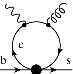
For inclusive decays one finds when integrating over the partonic phase space with GeV [352]. This estimate includes the numerically important correction. Note that the obtained is much larger than the estimate from electromagnetic penguins only .
An effect of similar size is found for decays using SCET, following from a nonfactorizable contribution suppressed by [486]. By dimensional arguments the estimate for the ratio is
| (86) |
Here is a dimensionless parameter of order one that depends on the final hadronic state . The second term remains in the limit of a massless light quark . Although power suppressed, it is enhanced by the large ratio . A dimensional estimate is thus , which would translate into an asymmetry () of about 10%, much larger than the LO estimate of that gives an asymmetry in transitions of around 3%. A more reliable estimate requires a challenging dynamical computation of the nonlocal nonfactorizable matrix element. However, these theoretical difficulties need not stand in the way of experimental progress as there is data driven method to separate the SM contamination by studying the dependence of the asymmetry on the final state [60] as we discuss below.
First steps in the direction of explicit model calculations find using QCD sum rules [122], consistent with the leading order estimate. In particular, expanding the relevant nonlocal operator in powers of and then keeping only the first term, they obtain for [see also [450]]
| (87) |
with parametrizing matrix elements of the nonlocal operator. Another calculation using pQCD obtained a very similar result for the asymmetry, [505].
Experimentally, the photon polarization can be measured from time dependent decay utilizing the interference of mixing with the right- and left-handed photon amplitudes [62, 60]. In particular, taking the time-dependent asymmetry summed over the unobserved photon polarization
| (88) |
the two coefficients are
| (89) |
where and . Note that when the “wrong” polarization amplitudes and vanish. This can be made more transparent in a simplified case where is a CP eigenstate with eigenvalue , while also assuming that the transitions are dominated by a single weak phase , so that and , where and are strong amplitudes. Then
| (90) |
and . Here as in Eq. (85). The asymmetry vanishes in the limit of 100% left-handed photon polarization ().
The value of depends crucially also on the mismatch between the weak phase of the decay amplitude and the mixing phases, and . There are two distinct categories. For and decays this phase difference is large () and is suppressed only by . For and decays, on the other hand, the weak phase difference vanishes so that in SM with negligible theoretical uncertainty. For NP to modify these predictions it has to induce large right-handed photon polarization amplitude, while for and decays also a new weak phase is needed to have .
Current results give a world average [130, 581, 104], and the first measurement of time-dependent asymmetries in decays has recently been reported, [582]. These are compatible, within experimental errors, with the SM predictions. A SFF could reduce the uncertainty on the former to about – and on the latter to about (see Table 12).
Measurements have also been made over an extended range of invariant mass in . In multibody exclusive radiative decays, a nonvanishing right-handed photon amplitude can be present at leading order in the expansion. However, using a combination of SCET and chiral perturbation theory (ChPT) methods applicable in kinematical region with one energetic kaon and a soft pion was found to be numerically less than 1% due to kinematical suppression [356, 357]. With the SFF data, the multibody radiative decays will be most useful to search for SM corrections to the photon polarization. These effects depend on the Dalitz plot position, in contrast to NP effects, which should be universal [60]. The LO dipole moment operator (as well as NP) would give rise to an asymmetry that is independent of the energy of the photon whereas the soft gluon effects will give rise to an asymmetry that depends on photon energy. Thus there is a model independent, completely data driven method to search for NP effects by studies of time dependent asymmetries. In addition, further decay modes, such as , and can also be used [61] in a very similar fashion.
Other approaches for probing the photon polarization in decays have been suggested and can be employed at a SFF. One powerful idea is to relate the photon polarization information to angular distributions of the final state hadrons. Examples relevant for a SFF are [364, 372], and [61, 539]. Similar tests have been suggested also using decays, such as [500, 350, 414, 415] and [478].
We consider decays, where the final hadronic state originates from the strong decay of resonance , produced in the weak decay . The lowest lying vector state, the , cannot be used for this purpose, since the polarization is not observable in its two-body decay . This is due to the fact that it is impossible to form a T-odd quantity from only two vectors, the photon momentum and the momentum, in the rest frame.
The photon polarization can then be measured through higher resonance decays. The angular distribution of the decay width in rest frame is [372]
| (91) |
Here is the angle between the direction opposite to the photon momentum () and the vector (the pions are ordered in terms of their momenta). The first three terms in Eq. (91) correspond respectively to decays through resonances with and , while the last terms come from – interference. The hadronic parameters can be computed from the Breit-Wigner resonant model [364, 372]. The resonance decays predominantly to . The relevant parameters in are then fixed by isospin, leading to a precise determination . Thus, measurements of the angular distribution Eq. (91) restricted to the mass range can be used to extract the photon polarization parameter . So far only an upper bound on exists [589]. The use of the narrow resonance , with a larger branching ratio [589, 98], may be more advantageous experimentally. A drawback is the estimate of in which a strong phase between and decay amplitudes needs to be obtained from an independent measurement.
The method outlined above works only for certain charge states, for which two channels interfere to produce the up-down asymmetry in . These channels are , where the interfering channels are and , and , where the interfering channels are and .
VIII.2 and decays
The rare decays form another class of FCNC processes, which proceed in the SM only through loop effects. The richer structure of the final state allows tests complementary to those performed in weak radiative decays. In addition to the total branching fraction, one can study also the dilepton invariant mass, the forward-backward asymmetry, and various polarization observables. We discuss these predictions, considering in turn the exclusive and inclusive channels.
VIII.2.1 Inclusive decays
In inclusive decays there are three distinct regions of dilepton invariant mass : (i) the low region, GeV2, (ii) the high region GeV2, and (iii) the charm resonance region GeV2. In the intermediate region (iii) resonances couple to the dilepton pair through a virtual photon, leading to nonperturbative strong interaction effects which are difficult to compute in a model independent way.
In the low and high regions, a model independent computation of the decay rate is possible using an OPE and heavy quark expansion, similar to that used for the rare radiative decays discussed in Section VIII.1.1. QCD corrections have been evaluated at NNLO including the complete three-loop mixing of the four quark operators into necessary for a complete solution of the RGE to NNLL order [53, 334, 335, 52, 322, 184, 428]. This calculation has been further improved by including electromagnetic log enhanced contributions that appear only if the integration over dilepton mass is restricted to a range but vanish for the full rate [428, 429, 184]. Nonperturbative power suppressed effects have been considered in [308, 37]. Effects of the intermediate states in the resonance region can be modeled assuming factorization of the four-quark operator [462].
Integrating over the low dilepton invariant mass range GeV2, the partial branching fractions corresponding to the low region are [429]
| (92) | |||||
| (93) |
where the dominant theoretical uncertainty arises from scale dependence, along with smaller uncertainties from the quark masses, CKM matrix elements, and nonperturbative corrections. The predictions agree well with the present average of the BABAR and Belle experimental measurements of this quantity [75, 441, 429] . The present (SM) theory error for the branching fraction is below the total experimental uncertainty. At a SFF the situation would be reversed.
Additional uncertainty in these predictions is introduced if a cut on the hadronic mass is imposed to eliminate charm backgrounds. This introduces sensitivity to the shape function, which however can be eliminated using data [474]. In the high region, an improvement in theory is possible, if the integrated decay rate is normalized to the semileptonic rate with the same cut [487]. This drastically reduces the size of and power corrections.
Besides the dilepton invariant mass spectrum the observable most often discussed is the forward-backward asymmetry. However, recently Lee et al. [475] pointed out that a third constraint can be obtained from double differential decay width
| (94) |
where , with the angle between and the meson three-momentum in the center-of-mass frame. The functions do not depend on . The sum gives the dilepton invariant mass spectrum , while the forward-backward asymmetry (FBA) is conventionaly defined as . The importance of the functions is that they are calculable in the low and high regions, and also depend differently on the Wilson coefficients of the effective weak Hamiltonian of Eq. (5). This suffices to determine the sizes and signs of all the relevant coefficients, probing in this way NP effects. At leading order they have a general structure [475]
| (95) |
where . The modified Wilson coefficients are independent linear combinations of the Wilson coefficients and in weak Hamiltonian of Eq. (5). They are related to the NNLO “effective” Wilson coefficients calculated in [53, 155, 335].


Note that in and the coefficient is enhanced by a pole so that measuring the dilepton mass dependence gives further information. Also, has a zero at . The existence of a zero of the FBA and the relative insensitivity to hadronic physics effects was first pointed out for exclusive channels [223], and subsequently extended also to the inclusive channels [39, 334]. In the SM the zero appears in the low region, sufficiently away from the charm resonance region to allow a precise computation of its position in perturbation theory. The value of the zero of the FBA is one of the most precisely calculated observables in flavor physics with a theoretical error at the order of . For , for instance, the improved NNLO prediction is [428], where the largest uncertainty is due to the remaining scale dependence (0.10). The position of the zero is directly related to the relative size and sign of the Wilson coefficients and . Thus it is very sensitive to new physics effects in these parameters. This quantity has not yet been measured, but estimates show that a precision of about could be obtained at a SFF [192, 404].
VIII.2.2 Exclusive and decays
The channels are experimentally cleaner than inclusive decays, but more complicated theoretically. The transition amplitude depends on hadronic physics through form factors. The theoretical formalism described in Sec. VIII.1.2 for exclusive radiative decays can be applied to this case as well.
The simplest are the decays with one pseudoscalar meson, such as or . Unlike decays that are not possible due to angular momentum conservation, the dilepton decays are allowed since the dilepton can carry zero helicity. Especially interesting for NP searches is the angular dependence on , the angle between the and the momenta in the dilepton rest frame. In the SM the dependence is simply . Allowing for scalar and pseudoscalar couplings to the leptons, which are possible in extensions of the SM, the general angular distribution is [182]
| (96) |
The coefficient receives contributions from the scalar and pseudoscalar couplings to the leptons, while depends on the interference between the vector and scalar couplings. As these terms vanish in the SM, their measurement is a null test sensitive to new physics from scalar and pseudoscalar penguins - see [185] for a detailed study. The first measurement of these parameters has been carried out in decays by BABAR [85]. The results are compatible with zero: and , where the first error is statistical and the second systematic. These measurements could become an order of magnitude more precise, and measure or set tight bounds on coefficients of NP operators which can produce these asymmetries.

We turn next to the decays with a vector meson in the final state, such as and . Since vector mesons carry a polarization, the final state has a more complex structure. The decays to , and the final state is specified by three angles defined as in Fig. 17. After integrating over the rate is described by three functions of as in the inclusive case, Eq. (95), with the difference that the Wilson coefficients are also multiplied by form factors. As in inclusive case, the transverse helicity amplitudes are dominated by the photon pole in the low region. In the high region, the terms dominate the amplitudes. Fig. 18 shows results for the decay rate and the FBA in the exclusive mode [155]. Due to form factor uncertainties the determination of the Wilson coefficients and the resulting NP constraints have substantially larger theoretical errors than the ones following from the inclusive decays (compare for instance Fig. 16 with Fig. 18).
In the large recoil limit the amplitudes satisfy factorization relations at leading order in [155, 142, 154, 412]. These factorization relations reduce the number of unknowns by expressing the amplitudes as combinations of soft overlap factors and factorizable contributions, multiplied with hard coefficients. The factorization relations predict that in the SM the right(left)-handed helicity amplitudes for are power suppressed. Any non-standard chirality structure could change this. A second prediction in the large recoil limit is that the left-handed helicity amplitude has a zero at dilepton invariant mass . In the SM this is predicted to be [155, 156]
| (97) |
This result was improved recently by including the resummation of the Sudakov logs in SCET [38], reducing the scale dependence uncertainty. The measurement of can be translated into a measurement of , up to a correction depending on the ratio of two form factors , which has been computed in factorization [155, 159]. Whether the soft overlap and the factorizable contributions in these form factors are comparable or not is still a subject of discussion, and may lead to larger errors than usually quoted in the literature [475]. Additional uncertainty can be introduced by the power corrections.


Various other observables are accessible in decays, including time-dependent [456] and transverse polarization asymmetries [461, 496]. These provide additional possibilities to probe the suppression of right-handed amplitudes and to search for NP operators with non-standard chirality at a SFF. We note the presence of possible SM contamination to these observables due to contributions to the right-handed amplitude in the multibody channel in the soft pion region [358]55 5 These contributions also introduce a shift in the position of the FBA zero in , as the is always observed through the final state.. This is similar to the effect discussed above for , and could be reduced by applying phase space cuts on the pion energy.
Further observables are accessible in the case with massive leptons, . The polarization asymmetry
| (98) |
integrated over the region , is about in the SM, but NP effects can change this prediction [409, 272]. No experimental studies of decays exist, making predictions of the SFF sensitivity unreliable. However, it appears that exclusive modes could be measured.
Another related mode is , mediated in the SM through the box and penguin diagrams, which are matched onto the operator . In extensions of the SM, additional diagrams can contribute, such as Higgs-mediated penguins in models with an extended Higgs sector, and models with modified couplings [387, 175]. The SM expectation for the branching fractions of these modes is [210], and . The dominant exclusive modes are , which are expected to occur with branching fractions of about . Present data give only an upper bound for at the level of [80, 246], which is one order of magnitude above the SM prediction. These modes are very challenging experimentally because of the presence of two undetected neutrinos. Nonetheless, the expected precision of the measurement of at a SFF is 20%, while the mode should be at the limit of observability [192].
VIII.3 Constraints on CKM parameters
The radiative are sensitive to the CKM elements involving the third generation quarks. In the following we briefly review the methods proposed for precision determination of the CKM parameters, and indicate the types of constraints which can be obtained.
from inclusive and : The inclusive radiative decays were discussed in Section VIII.1.1 and the inclusive semileptonic decays in Section V. For both types of the decays only part of the phase space is accessible experimentally. In semileptonic decays a cut on lepton energy or hadronic invariant mass needs to be made to avoid charm background, while in the photon needs to be energetic enough to reduce background. Experimentally accessible is the so called shape function region of the phase space, where the inclusive state forms an energetic jet with mass . Restricted to this region the OPE breaks down, while instead SCET is applicable. The decay widths factorize in a form shown in Eq. (74) for . Both radiative and semileptonic decays depend, at LO in , on the the same shape function describing the nonperturbative dynamics of the meson. The dependence on the shape function can be eliminated by combining the radiative and semileptonic rates. This then determines , with different methods of implementing the basic idea discussed in detail in Sec. V (see also a review by Paz [542] and recent developments in Lee [473]).
from : The radiative and amplitudes are dominated by electromagnetic penguin contributions proportional to and CKM elements respectively. The ratio of the charge-averaged rates is then
| (99) |
where , and for spectator quark flavors. The coefficient denotes the WA contribution in , while it is negligible for . The coefficient parameterizes the SU(3) breaking in the ratio of tensor form factors. The theory error in the determination of is thus due to these two coefficients. The coefficient can be calculated using factorization. Writing
| (100) |
Bosch and Buchalla [201] find for , and for . (For an alternative treatment, see Ball et al. [120].) The WA amplitude is larger for charged decays, where it is color allowed, in contrast to neutral decays, where it is color suppressed. Along with the above values of show that the uncertainty introduced by the WA contribution is minimal in neutral radiative decays.

The second source of theoretical uncertainty is given by SU(3) breaking. The parameter was estimated using QCD sum rules with the most recent result [123]. It seems rather difficult to improve on this calculation in a model independent way.
This method for determining has been used to obtain [9] and [93], where the first errors are experimental and the second theoretical, and in both cases the average over the channels is used. A dramatic improvement in experimental error can be expected at a SFF, and while the theoretical error can be reduced by using only the cleaner , the precision is likely to be limited at about due to the SU(3) breaking correction discussed above. This could possibly be improved using data collected at the , as discussed in Section IX.3.
from and : The ratio of CKM matrix elements can be constrained by combining the semileptonic mode with the radiative decay [201, 159]. In the large recoil limit the relevant form factors satisfy factorization relations.
The doubly differential semileptonic rate expressed in terms of the helicity amplitudes is
| (101) |
where is the angle between the and the meson momentum in the center of mass frame. At only the left-handed helicity amplitude contributes. The limit of the ratio of the partial rate to the rate depends only on
| (102) |
where is a tensor current form factor Eq. (84), while is calculable in a perturbative expansion in and . This ratio has been computed to be [159], allowing for a 60% uncertainty in the spectator-scattering contribution. This amounts to a 10% uncertainty on this determination of , which however does not include uncertainties from power suppressed contributions.
from and : In the low recoil region , the amplitude can be computed in an expansion in [355], relating it to the semileptonic decay , up to SU(3) breaking correction in the form factors. These can be eliminated using semileptonic decay rates by forming the Grinstein double ratio [488]
| (103) |
which is proportional to . The theory error on of this method is about 5%, but measurements of the required branching fractions in the region GeV2 require SFF statistics.
Constraints from the isospin asymmetry in : Assuming dominance by the penguin amplitude in , isospin symmetry relates the charged and neutral modes to be . The present experimental data point to a possible isospin asymmetry. The most recent world averages give [130, 93, 9] (using CP-conjugate modes)
| (104) | |||||
Several mechanisms can introduce a nonzero isospin asymmetry: i) the quark mass difference leading to isospin asymmetry in the tensor form factor ; ii) contributions from operators other than where the photon attaches to the spectator quark in the meson; iii) spectator diagrams such as those in Fig. 14, which depend on the spectator quark through its electric charge, and the hard scattering amplitude.
The dominant contribution to the isospin asymmetry in the SM is given by the last mechanism (iii), mediated by the four-quark operators . The matrix elements of these operators can be computed using factorization and the heavy quark expansion [451, 36, 354, 155, 200, 40]. Since the four-quark operators contribute with a different weak phase to the penguin amplitude, the result is sensitive to CKM parameters, in particular to the weak phase . Using as inputs the parameters from the CKM fit, an isospin asymmetry of a few percent is possible, with significant uncertainty from hadronic parameters [156]
| (105) |
This prediction can be turned around to obtain constraints on the CKM parameters , using the asymmetries. As discussed in [156], measurements of the direct CP asymmetry and of the isospin asymmetry in give complementary constraints, which in principle allow a complete determination of the CKM parameters. However, the precision of such a determination is ultimately going to be limited by hadronic uncertainties and power corrections.
IX physics at
The resonance is heavy enough that it decays both to and mesons. So far, several machines have operated at the resonance resulting in of data collected by the CLEO collaboration [166, 494], followed by of data collected by Belle collaboration during an engineering run [294] and a sample of about collected by Belle during a one month long run in June 2006. Baracchini et al. [127] performed a comprehensive analysis of the physics opportunities that would be offered by much larger data samples of () from a short (long) run of a SFF at the , where the data sample is recorded in special purpose runs. Collecting should require less than one month at a peak luminosity of . As a result, a SFF can give information on the system that is complementary to that from hadronic experiments. In Table 9 we give the expected precision from a SFF and LHCb for a sample of observables, clearly showing complementarity. In particular, the SFF can measure inclusive decays and modes with neutrals, which are inherently difficult in hadronic environment while LHCb provides superior time-dependent measurements of all-charged final states.
Physical processes involving mesons add to the wealth of information already available from the systems because the initial light quark is an quark. As a result, decays are sensitive to a different set of NP operators transforming between and generations than are decays of . The prime examples are where semileptonic operators are probed and – mixing where NP operators are probed. In addition, can improve knowledge of hadronic processes since and are related by U-spin. In the application of flavor SU(3) to hadronic matrix elements then the commonly used dynamical assumption of small annihilation-like amplitudes may no longer be needed.
| Observable | SFF () | SFF () | LHCb () |
|---|---|---|---|
| () | |||
| evidence | |||
| from | |||
IX.1 – mixing parameters
– mixing is described by the mass difference of the two eigenstates, the average of two decay widths and their difference , by and by the weak mixing phase , which is very small in the SM, [238], see also Eq. (38). All these parameters can be modified by NP contributions and are, for instance, very sensitive to the large regime of the MSSM as discussed in Section III.4.4.
The oscillation frequency has been measured recently [20], and is found to be consistent with SM predictions, within somewhat large theory errors. These oscillations are too fast to be resolved at a SFF, which thus cannot measure . However, measurements of the other parameters, , and are possible through time dependent untagged decay rates. Explicitly, for a pair produced from at the this is given by [297]
| (106) |
where is a CP-eigenstate and is given in Eq. (42). The normalization factor is given by , neglecting possible effects due to CP violation in mixing.
At the , CP-tagged initial states can also be used to extract the untarity angle rather cleanly [309, 68], and to constrain lifetime difference through time independent measurements [63].
The most promising channel for measuring – mixing parameters at a hadronic machine is , where angular analysis is needed to separate CP-even and CP-odd components. Recent measurements at D0 and CDF favor large making further studies highly interesting [1, 6]. As shown in Table 9 a SFF cannot compete with LHCb in this analysis, either for or for measurements, assuming systematic errors at LHCb are negligible. However, LHCb and a SFF can study complementary channels. For example, or from the penguin dominated , are difficult measurements at hadronic machines as shown in Table 9. The latter mode would be complementary to , where a precision of is expected after of data at LHCb (1 year of nominal luminosity running). Other interesting modes that can be studied at a SFF include , , , , and [192].
Another important observable is the semileptonic asymmetry , which is a measure of CP violation in mixing
| (107) |
The error on will become systematic dominated relatively soon. Taking as a guide the systematic error from current measurements at the , this will happen at an integrated luminosity of about at the . Thus systematics will saturate the error quoted in Table 9 for (where the statistical error is only ) [192]. Note that the LHCb estimate in Table 9 gives only the statistical error on , while systematic errors could be substantial due to the hadronic environment.
IX.2 Rare decays
One of the most important decays for NP searches is . In the SM this decay is chirally and loop suppressed with a branching fraction of [180]. Exchanges of new scalar particles can lift this suppression, significantly enhancing the rate. For instance, in the MSSM it is enhanced in the large regime (cf. Section III.4.4). After one year of nominal LHCb data taking evidence at the SM rate will be possible, while the SFF sensitivity to this channel is not competitive as indicated in Table 9.
A SFF can make a significant impact in radiative decays and decay modes with neutrals. One example is . Here the SM expectation is [556], while NP effects can significantly enhance the rate; for instance, the rate is enhanced by an order of magnitude in the parity violating MSSM [329]. The Belle sample of has already been used to demonstrate the potential of the SFF approach; the first observation of the penguin decay mode has recently been reported, along with a statistics limited upper limit on a factor of ten above the SM level [585].
IX.3 Improved determinations of and of
As described in Section VIII.3, exclusive radiative decays mediated by and penguins can be used to obtain constraints on the CKM ratio . An analogous treatment to that for can be applied to , where the theoretical error is expected to be reduced. This is due to the simple observation that the final states and are close in mass and are related by U-spin, which should help studies on the lattice. Moreover, a comparison of to offers a determination of that is free from SU(3) breaking corrections in the form factors [127, 192]. An improved determination of from radiative decays will be very helpful to compare to that from mixing, and with the SM fit.
Study of the inclusive and exclusive charmless semileptonic decays can play a very important role in an improved determination. For the lattice calculation of form factors a smaller extrapolation in valence light quark masses is needed than for form factors, reducing the errors. Since modes have significant branching ratios of , this can be an important early application of studies.
X Charm physics
There are many reasons for vigorously pursuing charm physics at a SFF. Perhaps most important is the intimate relation of charm to the top quark. Because of its large mass top quark is sensitive to NP effects in many models. New interactions involving the top quark quite naturally also imply modified interactions of the charm quark. For example, models of warped extra-dimensions, discussed in Section III.5, inevitably lead to flavor-changing interactions for the charm quark [26, 24, 312]. The same is true of two Higgs doublet models, in which the top quark has a special role [276, 588].
Charm also provides a unique handle on mixing effects in the up-type (charge ) sector. The top quark does not form bound states, which makes the only system where this study is possible. Importance of these studies is nicely illustrated by the constraint that they provide on the MSSM squark spectrum and mixing [531]. The squark-quark-gluino flavor violating coupling that mixes the first two generations is given by with for up (down) squarks. The difference of the two mixing angles needs to reproduce the Cabibbo angle
| (108) |
Small enough can sufficiently suppresses SUSY corrections to mixing even for nondegenerate squarks with TeV masses. This is possible in the absence of information on mixing. The smallness of mixing, however, requires that also is small, which violates the relation to the Cabibbo angle in Eq. (108). The squarks with masses light enough to be observable at LHC thus need to be degenerate [531].
We next summarize the salient aspects of charm physics – detailed reviews can be found in [167, 225, 51]. Within the SM, some aspects of the charm system are under excellent theoretical control. In particular, one expects negligible CP asymmetry in charm decays since the weak phase comes in CKM suppressed. The strong phases on the other hand are expected to be large in the charm region as it is rich with resonances. This means that a NP weak phase is likely to lead to observable CP violation. Moreover, although the absolute size of mixing cannot be reliably calculated in the SM because of long distance contamination, the rate of mixing can be used to put bounds on NP parameters in many scenarios [341]. Furthermore, the indirect CP violation is negligibly small in the SM. It arises from a short distance contribution that is subleading in – mixing compared to the long distance piece and is furthermore CKM suppressed by . It therefore provides a possibility for a very clear NP signal.
The most promising modes to search for direct CP violation in charm decays are singly Cabibbo suppressed channels, such as , , , , which in the SM receive contributions from two weak amplitudes, tree and penguin [384]. As already mentioned indirect CP violation is very small, while direct CP violation is both loop and CKM suppressed making it negligible as well. Supersymmetric squark-gluino loops on the other hand can saturate the present experimental sensitivity of [384]. Doubly Cabibbo suppressed modes may also be useful in the search for NP effects since the SM cannot give rise to any direct CP violation and thus the SM “background” contribution is small.
The prospects for finding a BSM CP-odd phase via oscillations dramatically improved in 2007. Using time-dependent measurements from their large charm data samples, Belle and BABAR reported the first evidence for – mixing [573, 94]. As discussed above the existence of mixing makes it possible to search for new physics (CP-odd) phases in the charm sector via CP-violating asymmetries.
The phase of mixing, is the analogue of the phases of mixing or mixing discussed in Section IV.66 6 Here we assume that any large phase is due to new physics. In this case, the quantity that is measured is the phase of mixing via . In the SM, it is possible that in which case the relation between the experimental phase and the phase of mixing is more complicated. While the phase of mixing is large in the SM, the phases of mixing and mixing are small in the SM; both are examples of null tests, with the phase of mixing particularly clean since it is expected to be of order in the SM. We emphasise that new physics that appears in the sector (involving up-type quarks) may be completely different from that in the sector.
Currently, the best sensitivity on , of , is obtained from time-dependent Dalitz plot analysis [10]. Assuming that there are no fundamental systematic limitations in the understanding of this Dalitz plot structure, the sensitivity to at a SFF will be about –. The use of other modes such as and can improve the overall sensitivity and help to eliminate ambiguous solutions for the phase [568].
Searches for CP-violation via triple correlations are also very powerful. These searches require final states that contain several linearly independent 4-momenta and/or spins. A crucial advantage is that this class of somewhat complicated final states does not require the presence of a CP-conserving (rescattering) phase; in odd-observables the CP asymmetry is proportional to the real part of the Feynman amplitude [55]. Many final states such as , , and can be used; initial studies of some of these have been carried out [489]. Semi-leptonic rare decays are of special interest as their small branching fractions can translate into large CP-asymmetries. In practice, the search for triple correlations requires the presence of a term in the angular distribution that is proportional to , where is the angle between the planes of the two pseudoscalars and the two leptons. It has recently been pointed out by Bigi [168] that this asymmetry could be enhanced using data taken by a SFF in the charm energy region (i.e. at the resonance). In this scenario, one uses the process followed by tagging of the short-lived state via, e.g., . This then allows analysis of the decay. The operation of a SFF at the resonance would also provide important input to the determination of from decays, as discussed in Section IV.2 [571, 366, 70, 195, 196].
CP violation in mixing can be probed using inclusive semileptonic CP asymmetry of “wrong sign” leptons [168]:
| (109) | |||||
A nonnegligible value requires a BSM CP violating phase in dynamics and depends on both and . In the system, while and are both small, the ratio need not be. In fact the central values in the present data are consistent with unity or even a somewhat bigger value. The asymmetry is driven by this ratio or its inverse, whichever is smaller. Thus although the rate for “wrong sign” leptons is small, their CP asymmetry might not be if there is a significant NP phase [168]. Due to the smallness of the rate for “wrong sign” leptonic decays, NP constraints from this measurement would still be statistics limited at a SFF.
Finally, although we have focused on CP violation phenomena in this section, there is also a number of rare decays that can be useful probes of new physics effects. For example, searches for lepton flavor violating charm decays such as or , where is a light meson such as or , can clearly help improve the bounds on exotica. In addition, studies of decays provide complementary information to leptonic decays (discussed in Section III.3), and are useful to bound charged Higgs contributions in the large limit [558, 31, 32].
XI NP tests in the tau lepton sector
XI.1 Searches for Lepton Flavor Violation
The discovery of neutrino oscillations [281, 318, 27, 298, 42, 444] provides direct experimental evidence that the accidental lepton flavor symmetries of the renormalizable Standard Model are broken in nature. It is therefore compelling to search for lepton flavor violation (LFV) also in the decays of charged leptons. LFV decays of tau leptons can be searched for at a Super Flavor Factory. The list of interesting LFV modes includes , and , where stands for or , while the hadronic final state can be, for example, , , or a multihadronic state. These searches will complement studies of LFV in the muon sector. The decay will be searched for at MEG [349, 557], while conversion will be searched for at PRISM/PRIME [466, 561]. Another interesting way to search for NP effects is to test lepton flavor universality in vs. decays. The decays into muons can be well measured in hadronic environment, while the electron decays are easier to measure at a SFF. The current and expected future sensitivities of several LFV modes of interest are summarized in Table 10 (for more details, see Raidal et al. [550]).
| Mode | Current UL | Future UL/SES |
|---|---|---|
| — | ||
Extending to the leptonic sector the concept of minimal flavor violation, described in Section III.2, provides an effective field theory estimate of LFV [258, 351, 279]. The minimal lepton flavor violation (MLFV) hypothesis supposes that the scale at which the total lepton number gets broken is much larger than the mass scale of the lightest new particles extending the SM leptonic sector [258]. These new particles could, for instance, be the sleptons of MSSM. The assumption of MLFV is that the new particles break flavor minimally, i.e. only through charged lepton and neutrino Yukawa matrices.
MLFV predictions have several sources of theoretical uncertainties. First, unlike the quark sector the MFV prescription is not unique for the leptons because of the ambiguity in the neutrino sector. The minimal choice for the SM neutrino mass term is
| (110) |
with a spurion of MLFV. This mass term could arise from integrating out heavy right-handed neutrinos. In this case there is an additional spurion from heavy neutrino-light neutrino Yukawa terms with . This then changes the spurion analysis, giving different predictions on the size of LFV processes. Further ambiguities are due to unknown absolute size of neutrino masses, i.e. whether neutrinos have normal or inverted mass hierarchy, and from the size of CP violation in the leptonic sector. Most importantly, the minimal size of LFV effects is not fixed. Rescaling simultaneously the coupling matrix and the lepton number violation scale does not change the neutrino mass matrix, while it changes (keeping fixed at the same time). The rates of the lepton flavor violating processes therefore increase as the masses of the heavy neutrinos are raised77 7 They do decrease with increased , the mass scale of low energy NP particles (such as slepton), as for the most NP sensitive measurements.. This dependence cancels in the ratio . Normalizing to the charged-current decay
| (111) |
Cirigliano et al. [258] obtain that depending on the value of angle, with smaller values of obtained for smaller values of . Saturating the present experimental bound on at gives , within the reach of a SFF.
A working example of MLFV model is for instance the CMSSM with three right-handed neutrinos [47]. The correlations between and are shown in Fig. 21. In this scenario the rate for decay depends strongly on the value of the neutrino mixing parameter , and could be hard to measure if , whereas is approximately independent of this parameter. For the choices of parameters used in Fig. 21, based on the Snowmass point 1 [43], the rates of LFV processes are suppressed – much larger rates for are possible for other choices of NP parameters. Large LFV effects in charged lepton decays are found in other examples of extending SM with heavy right-handed neutrinos with or without supersymmetry [199, 545, 434, 504, 419, 301, 116, 22].

Embedding MFV in a GUT setup can lead to qualitatively different conclusions. Now the effective weak Hamiltonian for processes involves also the quark Yukawa couplings . This means that contrary to the MLFV case above, the and rates cannot be arbitrarily suppressed by lowering . For GeV the GUT induced contribution controlled by starts to dominate, which in turn for NP scale TeV gives above within reach of the MEG experiment [349]. The MLFV and GUT-MFV scenarios can be distinguished by comparing different and LFV rates. For instance, in the limit where quark-induced terms dominate one has and , with , giving , which allows to be just below the present exclusion bound. Further information that distinguishes the two scenarios can be obtained from , , and decays [257]. Explicit realizations of LFV in supersymmetric GUT models have been discussed in the literature [132, 133, 342, 229].
Similarly, correlations between different and decays for a general 2HDM have been derived [541, 540]. The decays and were found to be the most sensitive probes that can be close to present experimental bounds, while correlations between different decays are a signature of the theory.
In supersymmetric extensions of the SM, the dipole operator typically dominates over the four-lepton operators, which leads to a simple prediction [207]
| (112) |
If the off-diagonal slepton mass-matrix element and are large enough, the Higgs-mediated transitions can alter this conclusion. For instance in the decoupling limit [541]
| (113) |
In Little Higgs Models with -parity on the other hand, and box-diagram contributions dominate over the radiative operators, which then gives distinctly different ratios of decay widths to those in the MSSM, as shown in Table 11 [178]. In Little Higgs Models with -parity with a NP scale GeV, the LFV decays can be seen at a SFF. In other models , or can be enhanced [268, 559, 177, 564, 207, 485, 243, 348]. Further information on the LFV origin could be provided from Dalitz plot analysis of with large enough data samples [277, 506].
| Ratio | LHT | MSSM (dipole) | MSSM (Higgs) |
|---|---|---|---|
| 0.4–2.5 | |||
| 0.4–2.3 | |||
| 0.4–2.3 | 0.06–0.1 | ||
| 0.3–1.6 | 0.02–0.04 | ||
| 0.3–1.6 | |||
| 1.3–1.7 | 0.3–0.5 | ||
| 1.2–1.6 | 5–10 | ||
| – | 0.08–0.15 |
XI.2 Tests of lepton flavor universality in tau decays
A complementary window to NP is provided by precise tests of lepton flavor universality in charged current and decays. In the large regime of MSSM the deviations arise from Higgs-mediated LFV amplitudes, where the effects are generated by LF-conserving but mass dependent couplings. This is complementary to and decays, where deviations are mainly due to LFV couplings [439, 503].
It is important to note that, while most of the supersymmetric models discussed above were minimally flavor violating, this is far from being the only possibility still allowed by the LFV data. To first approximation the rare flavor changing charged lepton decays constrain the following combination of supersymmetric parameters
| (114) |
where is the slepton mixing angle with the generation indices, while and are the difference and the average of slepton masses, while for simplicity we suppress the indices for left-handed and right-handed sleptons. Thus the flavor bounds can be obeyed either if the mixing angles are small or if the sleptons are mass degenerate. Interpolation between the two options exemplifies a set of realistic supersymmetric models discussed by Feng et al. [311], where supersymmetry breaking mechanism was taken to be a combination of gauge mediated (leading to degeneracy) and gravity mediated supersymmetry breaking supplemented with horizontal symmetries (leading to alignment with split mass spectrum).
The high processes at LHC experiments probe a different combination of FV supersymmetric couplings. For degenerate sleptons with large mixing one may observe oscillations in or decay chains. This constrains (taking the limit of both sleptons having the same decay width for simplicity) [48]
| (115) |
which should be compared with Eq. (114). An example of constraints coming from the LHC and based on a preliminary simulation in the cMSSM is shown in Fig 22. A qualitatively similar interplay of LHC and SFF constraints is expected for . By having both the LHC high and low energy LFV measurements at high enough precision one is able to measure both the mixing angle and the mass splitting of the leptons, thus probing the nature of the supersymmetry breaking mechanism.
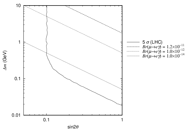
On the experimental side, a SFF is an ideal experiment to study lepton flavor violating tau decays due to the large cross-section ( at [126]) and a clean environment. It has much better sensitivity than the LHC experiments even for the apparently favourable channel [560, 579].
The factories have demonstrated the enormous potential for tau physics from an collider running at the . The current experimental upper limits for most lepton flavor violating tau decays are at present in the – range [407, 16, 95, 110, 516, 515, 15], indicating that a SFF will probe what is phenomenologically a highly interesting range, up to two orders of magnitude below the existing bounds.
For many of the LFV channels, the only limitation is due to statistics – there are no significant backgrounds as the process provides a very distinctive signature, and the neutrinoless final state allows the four-momentum of the decaying tau lepton to be reconstructed. In the limit of negligible background, the achievable upper limit scales with the integrated luminosity.
Special consideration must be given to the radiative decays and , since for these channels there is an important background source from SM tau decays (eg. ) combined with a photon from initial state radiation. This irreducible background is already an important factor in the current analyses [407, 79, 90], and will be dominant at very high luminosities. Control of these backgrounds and other improvements in the analyses will have an important effect on the ultimate sensitivity of a SFF to lepton flavor violating tau decays.
XI.3 CP Violation in the system
An observation of CP violation in decays would provide an incontrovertible NP signal. Several NP models allow direct CP violation effects in hadronic decays [382, 465, 286, 280, 285, 278], where the only SM background is that from daughter neutral kaons [169, 228] and is in . Partial rate asymmetries, integrated over the phase space for the decay, can be measured with subpercent precision at a SFF. A more comprehensive analysis requires a study of the amplitude structure functions [463, 464, 192]; these analyses can also be performed, but benefit from having a polarized beam to provide a reference axis.
A polarized beam can also be used to make measurements of the electric and magnetic dipole moments. For the EDM measurement, an improvement of three orders of magnitude on the present bounds [435] can be achieved [163]. However this range can be saturated only by exotic NP models that can avoid stringent bound on the electric dipole moment of the electron. For the MDM, the anomalous moment could be measured for the first time at a SFF [162].
XII Comparison of a Super Flavor Factory with LHCb
Since a Super Flavor Factory will take data in the LHC era, it is reasonable to ask how its physics reach compares with the flavor physics potential of the LHC experiments, most notably LHCb [521, 230]. By 2014, the LHCb experiment is expected to have accumulated of data from collisions at a luminosity of [212]. Moreover, LHCb is planning an upgrade where they would run at 10 times the initial design luminosity and record a data sample of about [520, 290].
The most striking outcome of any comparison between a SFF and LHCb is that the strengths of the two experiments are largely complementary. For example, the large boost of the hadrons produced at LHCb allows time-dependent studies of the oscillations of mesons while many of the measurements that constitute the primary physics motivation for a SFF cannot be performed in a high multiplicity hadronic environment, for example, rare decay modes with missing energy such as and . Measurements of the CKM matrix elements and and inclusive analyses of processes such as and also benefit greatly from the clean and relatively simple collider environment. At LHCb the reconstruction efficiencies are reduced for channels containing several neutral particles and for studies where the decay vertex must be determined from a meson. Consequently, a SFF has unique potential to measure the photon polarization via mixing-induced CP violation in . Similarly, a SFF is well placed to study possible NP effects in hadronic penguin decays as it can measure precisely the CP asymmetries in many decay modes including , , and . While LHCb will have limited capability for these channels, it can perform complementary measurements using decay modes such as and for radiative and hadronic transitions, respectively [230].
Where there is overlap, the strength of the SFF programme in its ability to use multiple approaches to reach the objective becomes apparent. For example, LHCb should be able to measure to about precision using [521], but will not be able to access the full information in the and channels, which is necessary to reduce the uncertainty to the – level of a SFF. Similarly, LHCb can certainly measure through mixing-induced CP violation in decay to high accuracy (about 0.01), but will have less sensitivity to make important complementary measurements (e.g., in and ). While LHCb hopes to measure the angle with a precision of –, extrapolations from current B factories show that a SFF is likely to be able to improve this precision to about . LHCb can probably make a precise measurement of the zero of the forward-backward asymmetry in , but a SFF can also measure the inclusive channel , which, as discussed in Section VIII.2.1 is theoretically a much cleaner and more powerful observable. The broader programme of a SFF thus provides a very comprehensive set of measurements in addition to its clean experimental environment and superior neutral detection capabilities. This will be of great importance for the study of flavor physics in the LHC era.
XIII Summary
| Observable | SFF sensitivity | Current sensitivity |
|---|---|---|
| () | 0.005–0.012 | 0.025 |
| () | 1–2∘ | (CKMfitter) |
| (, , ) | 1–2∘ | (CKMfitter) |
| (excl) | 3–5% | (PDG review) |
| (incl) | 3–5% | (PDG review) |
| 1.7–3.4% | ||
| 0.7–1.7% | ||
| 0.02–0.03 | 0.17 | |
| 0.01–0.02 | 0.07 | |
| 0.02–0.03 | 0.20 | |
| 3–4% | 30% | |
| 5–6% | not measured | |
| 2–2.5% | 31% | |
| 0.004–0.005 | 0.037 | |
| 0.01 | 0.12 | |
| 5–10% | ||
| 3–4% | 16% | |
| 0.02–0.03 | 0.24 | |
| 0.08–0.12 | 0.67 | |
| 4–6% | 23% | |
| 4–6% | not measured | |
| 16–20% | not measured | |
| 1–2∘ | ||
| 2–8 | not seen, | |
| 0.2–1 | not seen, – | |
| 0.4–4 | not seen, |
In this review we have summarized the physics case for a Super Flavor Factory (SFF); our emphasis has been on searches for New Physics. Such a high luminosity machine (integrating 50-75 ) will of course be a Super Factory, but importantly has enormous potential for exposing New Physics not only in the sector, but also in charm as well as in lepton decays.
In physics the range of clean and powerful observables is very extensive, see Table 12. A quick inspection vividly shows that the SFF will extend the current reach from the factories for many important observables by over an order of magnitude. Specifically, we should be able to significantly improve the precision with which we can cleanly measure the angles “directly” and also determine sides of the unitarity triangle enhancing our knowledge of these fundamental parameters of the SM as well as checking for new physics effects in mixing and in transitions. In addition, there are critically important direct searches for New Physics that are also possible. For example, we should be able to measure from penguin-dominated modes with an accuracy of a few percent. This will either clearly establish the presence of a new CP-odd phase in transitions or allow us to constrain it significantly. Improved measurements of direct and time-dependent CP asymmetries in a host of modes and the first results on the zero crossing of the forward-backward asymmetries in inclusive radiative decays will be exciting and extremely informative. Furthermore, a large class of null tests will either constrain NP or reveal its presence.
While the dramatic increase in luminosity at a SFF will allow significant improvements in many important existing measurements, the SFF also will provide an important step change over the factories in that many new channels and observables will become accessible for the first time. These include , and semi-inclusive hadronic modes. In addition, sensitive probes of right-handed currents will become possible through measurements of time-dependent asymmetries in radiative processes such as , as well as transverse polarization of the in semitauonic decays of mesons. At the SFF, the high statistics and kinematic constraints of production at the also will allow clean studies of many important inclusive processes in the recoil of fully reconstructed tagged mesons.
High luminosity charm studies will also be sensitive to the effects of new physics; the most important of these is a search for a new CP-odd phase in mixing () with a sensitivity of a few degrees. Improved studies of lepton flavor violation in decays with much higher sensitivities could also prove to be extremely important in revealing new phenomena or allowing us to constrain it more effectively.
A Super Flavor Factory will complement dedicated flavor studies at the LHC with its sensitivity to decay modes with photons and multiple neutrinos as well as inclusive processes. The SFF will extend the reach of the high experiments at the LHC in many ways and will help us interpret whatever type of New Physics is discovered there.
Acknowledgements.
We thank Rafael Porto for useful discussions and Sebastian Jaeger and Tobias Hurth for comments on the manuscript. Research supported in part by the US Department of Energy, contracts DE-FG02-04ER41291 (Hawaii) and DE-AC02-98CH10886 (BNL). The work of J. Z. was supported in part by the European Commission RTN network, Contract No. MRTN-CT-2006-035482 (FLAVIAnet) and by the Slovenian Research Agency.References
- [1] Aaltonen, T., et al. (CDF), 2007a, eprint arXiv:0712.2397 [hep-ex].
- [2] Aaltonen, T., et al. (CDF), 2007b, eprint arXiv:0712.1708 [hep-ex].
- [3] Abashian, A., et al., 2002, Nucl. Instrum. Meth. A479, 117.
- [4] Abazov, V. M., et al. (D0), 2005, Phys. Rev. Lett. 95, 171801.
- [5] Abazov, V. M., et al. (D0), 2007, Phys. Rev. D76, 092001.
- [6] Abazov, V. M., et al. (D0), 2008, eprint arXiv:0802.2255 [hep-ex].
- [7] Abbiendi, G., et al. (OPAL), 2001, Phys. Lett. B520, 1.
- [8] Abe, K., et al. (Belle), 2005, Phys. Rev. D71, 072003.
- [9] Abe, K., et al. (Belle), 2006a, Phys. Rev. Lett. 96, 221601.
- [10] Abe, K., et al. (Belle), 2007a, Phys. Rev. Lett. 99, 131803.
- [11] Abe, K., et al. (Belle), 2007b, Phys. Rev. Lett. 99, 121601.
- [12] Abe, K., et al. (Belle), 2007c, eprint arXiv:0708.1845 [hep-ex].
- [13] Abe, K., et al. (Belle), 2007d, Phys. Rev. D76, 091103.
- [14] Abe, K., et al. (Belle), 2007e, Phys. Rev. Lett. 98, 181804.
- [15] Abe, K., et al. (Belle), 2007f, eprint arXiv:0708.3276 [hep-ex].
- [16] Abe, K., et al. (Belle), 2008, Phys. Lett. B660, 154.
- [17] Abe, M., et al. (KEK-E246), 2004, Phys. Rev. Lett. 93, 131601.
- [18] Abe, M., et al., 2006b, Phys. Rev. D73, 072005.
- [19] Abe, T., et al., 2007g, eprint arXiv:0706.3248 [physics.ins-det].
- [20] Abulencia, A., et al. (CDF), 2006, Phys. Rev. Lett. 97, 242003.
- [21] Acosta, D. E., et al. (CDF), 2005, Phys. Rev. Lett. 94, 101803.
- [22] Agashe, K., A. E. Blechman, and F. Petriello, 2006, Phys. Rev. D74, 053011.
- [23] Agashe, K., A. Delgado, M. J. May, and R. Sundrum, 2003, JHEP 08, 050.
- [24] Agashe, K., M. Papucci, G. Perez, and D. Pirjol, 2005a, eprint hep-ph/0509117.
- [25] Agashe, K., G. Perez, and A. Soni, 2004, Phys. Rev. Lett. 93, 201804.
- [26] Agashe, K., G. Perez, and A. Soni, 2005b, Phys. Rev. D71, 016002.
- [27] Ahmad, Q. R., et al. (SNO), 2002, Phys. Rev. Lett. 89, 011301.
- [28] Ahmed, M., et al. (MEGA), 2002, Phys. Rev. D65, 112002.
- [29] Aihara, H., et al., 2006, Nucl. Instrum. Meth. A568, 269.
- [30] Akai, K., and Y. Morita, 2003, kEK-PREPRINT-2003-123.
- [31] Akeroyd, A. G., 2004, Prog. Theor. Phys. 111, 295.
- [32] Akeroyd, A. G., and C. H. Chen, 2007, Phys. Rev. D75, 075004.
- [33] Akeroyd, A. G., et al. (SuperKEKB Physics Working Group), 2004, eprint hep-ex/0406071.
- [34] Aleksan, R., B. Kayser, and D. London, 1994, Phys. Rev. Lett. 73, 18.
- [35] Aleksan, R., T. C. Petersen, and A. Soffer, 2003, Phys. Rev. D67, 096002.
- [36] Ali, A., and V. M. Braun, 1995, Phys. Lett. B359, 223.
- [37] Ali, A., G. Hiller, L. T. Handoko, and T. Morozumi, 1997, Phys. Rev. D55, 4105.
- [38] Ali, A., G. Kramer, and G.-h. Zhu, 2006, Eur. Phys. J. C47, 625.
- [39] Ali, A., E. Lunghi, C. Greub, and G. Hiller, 2002, Phys. Rev. D66, 034002.
- [40] Ali, A., and A. Y. Parkhomenko, 2002, Eur. Phys. J. C23, 89.
- [41] Ali, A., et al., 2007, Phys. Rev. D76, 074018.
- [42] Aliu, E., et al. (K2K), 2005, Phys. Rev. Lett. 94, 081802.
- [43] Allanach, B. C., et al., 2002, eprint hep-ph/0202233.
- [44] Andersen, J. R., and E. Gardi, 2006, JHEP 01, 097.
- [45] Antaramian, A., L. J. Hall, and A. Rasin, 1992, Phys. Rev. Lett. 69, 1871.
- [46] Antonio, D. J., et al. (RBC), 2008, Phys. Rev. Lett. 100, 032001.
- [47] Antusch, S., E. Arganda, M. J. Herrero, and A. M. Teixeira, 2006, JHEP 11, 090.
- [48] Arkani-Hamed, N., H.-C. Cheng, J. L. Feng, and L. J. Hall, 1996, Phys. Rev. Lett. 77, 1937.
- [49] Arnesen, C. M., Z. Ligeti, I. Z. Rothstein, and I. W. Stewart, 2006, eprint hep-ph/0607001.
- [50] Arnesen, M. C., B. Grinstein, I. Z. Rothstein, and I. W. Stewart, 2005, Phys. Rev. Lett. 95, 071802.
- [51] Artuso, M., B. Meadows, and A. A. Petrov, 2008, eprint arXiv:0802.2934 [hep-ph].
- [52] Asatrian, H. M., K. Bieri, C. Greub, and A. Hovhannisyan, 2002, Phys. Rev. D66, 094013.
- [53] Asatryan, H. H., H. M. Asatrian, C. Greub, and M. Walker, 2002, Phys. Rev. D65, 074004.
- [54] Athar, S. B., et al. (CLEO), 2003, Phys. Rev. D68, 072003.
- [55] Atwood, D., S. Bar-Shalom, G. Eilam, and A. Soni, 2001a, Phys. Rept. 347, 1.
- [56] Atwood, D., B. Blok, and A. Soni, 1996, Int. J. Mod. Phys. A11, 3743.
- [57] Atwood, D., I. Dunietz, and A. Soni, 1997a, Phys. Rev. Lett. 78, 3257.
- [58] Atwood, D., I. Dunietz, and A. Soni, 2001b, Phys. Rev. D63, 036005.
- [59] Atwood, D., G. Eilam, and A. Soni, 1993, Phys. Rev. Lett. 71, 492.
- [60] Atwood, D., T. Gershon, M. Hazumi, and A. Soni, 2005, Phys. Rev. D71, 076003.
- [61] Atwood, D., T. Gershon, M. Hazumi, and A. Soni, 2007, eprint hep-ph/0701021.
- [62] Atwood, D., M. Gronau, and A. Soni, 1997b, Phys. Rev. Lett. 79, 185.
- [63] Atwood, D., and A. A. Petrov, 2005, Phys. Rev. D71, 054032.
- [64] Atwood, D., L. Reina, and A. Soni, 1997c, Phys. Rev. D55, 3156.
- [65] Atwood, D., and A. Soni, 1997, Phys. Rev. Lett. 79, 5206.
- [66] Atwood, D., and A. Soni, 1998a, Phys. Rev. D58, 036005.
- [67] Atwood, D., and A. Soni, 1998b, Phys. Rev. Lett. 81, 3324.
- [68] Atwood, D., and A. Soni, 2002, Phys. Lett. B533, 37.
- [69] Atwood, D., and A. Soni, 2003a, Phys. Rev. D68, 033009.
- [70] Atwood, D., and A. Soni, 2003b, Phys. Rev. D68, 033003.
- [71] Atwood, D., and A. Soni, 2005, Phys. Rev. D71, 013007.
- [72] Aubert, B., et al. (BABAR), 2002, Nucl. Instrum. Meth. A479, 1.
- [73] Aubert, B., et al. (BABAR), 2003, Phys. Rev. Lett. 91, 051801.
- [74] Aubert, B., et al. (BABAR), 2004a, Phys. Rev. D70, 112006.
- [75] Aubert, B., et al. (BABAR), 2004b, Phys. Rev. Lett. 93, 081802.
- [76] Aubert, B., et al. (BABAR), 2004c, Phys. Rev. Lett. 93, 021804.
- [77] Aubert, B., et al. (BABAR), 2005a, Phys. Rev. D71, 051502.
- [78] Aubert, B., et al. (BABAR), 2005b, Phys. Rev. D72, 052004.
- [79] Aubert, B., et al. (BABAR), 2005c, Phys. Rev. Lett. 95, 041802.
- [80] Aubert, B., et al. (BABAR), 2005d, Phys. Rev. Lett. 94, 101801.
- [81] Aubert, B., et al. (BABAR), 2006a, Phys. Rev. Lett. 96, 221801.
- [82] Aubert, B., et al. (BABAR), 2006b, Phys. Rev. Lett. 97, 171803.
- [83] Aubert, B., et al. (BABAR), 2006c, eprint hep-ex/0607104.
- [84] Aubert, B., et al. (BABAR), 2006d, Phys. Rev. D73, 012004.
- [85] Aubert, B., et al. (BABAR), 2006e, Phys. Rev. D73, 092001.
- [86] Aubert, B., et al. (BABAR), 2006f, eprint hep-ex/0607101.
- [87] Aubert, B., et al. (BABAR), 2006g, Phys. Rev. D74, 092004.
- [88] Aubert, B., et al. (BABAR), 2006h, Phys. Rev. Lett. 97, 171805.
- [89] Aubert, B., et al. (BABAR), 2006i, eprint hep-ex/0607053.
- [90] Aubert, B., et al. (BABAR), 2006j, Phys. Rev. Lett. 96, 041801.
- [91] Aubert, B., et al. (BABAR), 2007a, Phys. Rev. D76, 052002.
- [92] Aubert, B., et al. (BABAR), 2007b, Phys. Rev. D76, 031103.
- [93] Aubert, B., et al. (BABAR), 2007c, Phys. Rev. Lett. 98, 151802.
- [94] Aubert, B., et al. (BABAR), 2007d, Phys. Rev. Lett. 98, 211802.
- [95] Aubert, B., et al. (BABAR), 2007e, Phys. Rev. Lett. 99, 251803.
- [96] Aubert, B., et al. (BABAR), 2007f, Phys. Rev. Lett. 99, 171803.
- [97] Aubert, B., et al. (BABAR), 2007g, Phys. Rev. D75, 012008.
- [98] Aubert, B., et al. (BABAR), 2007h, Phys. Rev. Lett. 98, 211804.
- [99] Aubert, B., et al. (BABAR), 2007i, Phys. Rev. Lett. 99, 231802.
- [100] Aubert, B., et al. (BABAR), 2007j, Phys. Rev. D76, 091101.
- [101] Aubert, B., et al. (BABAR), 2007k, Phys. Rev. D76, 071101.
- [102] Aubert, B., et al. (BABAR), 2007l, Phys. Rev. D76, 012004.
- [103] Aubert, B., et al. (BABAR), 2007m, Phys. Rev. Lett. 98, 091801.
- [104] Aubert, B., et al. (BABAR), 2007n, eprint arXiv:0708.1614 [hep-ex].
- [105] Aubert, B., et al. (BABAR), 2007o, Phys. Rev. Lett. 99, 161802.
- [106] Aubert, B., et al. (BABAR), 2007p, eprint arXiv:0708.3702 [hep-ex].
- [107] Aubert, B., et al. (BABAR), 2007q, Phys. Rev. Lett. 98, 031801.
- [108] Aubert, B., et al. (BABAR), 2007r, Phys. Rev. Lett. 99, 021603.
- [109] Aubert, B., et al. (BABAR), 2007s, eprint arXiv:0709.1698 [hep-ex].
- [110] Aubert, B., et al. (BABAR), 2007t, Phys. Rev. Lett. 98, 061803.
- [111] Aubert, B., et al. (BABAR), 2007u, Phys. Rev. D76, 091102.
- [112] Aubert, B., et al. (BABAR), 2007v, eprint arXiv:0708.1630 [hep-ex].
- [113] Aubert, B., et al. (BABAR), 2007w, eprint arXiv:0708.2097 [hep-ex].
- [114] Aubert, B., et al. (BABAR), 2008a, Phys. Rev. D77, 011107.
- [115] Aubert, B., et al. (BABAR), 2008b, Phys. Rev. D77, 012003.
- [116] Babu, K. S., and C. Kolda, 2002, Phys. Rev. Lett. 89, 241802.
- [117] Babu, K. S., and C. F. Kolda, 2000, Phys. Rev. Lett. 84, 228.
- [118] Baek, S., P. Hamel, D. London, A. Datta, and D. A. Suprun, 2005, Phys. Rev. D71, 057502.
- [119] Ball, P., 2006, eprint hep-ph/0612190.
- [120] Ball, P., G. W. Jones, and R. Zwicky, 2007, Phys. Rev. D75, 054004.
- [121] Ball, P., and R. Zwicky, 2005, Phys. Rev. D71, 014029.
- [122] Ball, P., and R. Zwicky, 2006a, Phys. Lett. B642, 478.
- [123] Ball, P., and R. Zwicky, 2006b, JHEP 04, 046.
- [124] Bander, M., D. Silverman, and A. Soni, 1979, Phys. Rev. Lett. 43, 242.
- [125] Bander, M., D. Silverman, and A. Soni, 1980, Phys. Rev. Lett. 44, 7, [Erratum-ibid. 44, 962 (1980)].
- [126] Banerjee, S., B. Pietrzyk, J. M. Roney, and Z. Was, 2007, eprint arXiv:0706.3235 [hep-ph].
- [127] Baracchini, E., et al., 2007, JHEP 08, 005.
- [128] Baranowski, K., and M. Misiak, 2000, Phys. Lett. B483, 410.
- [129] Barate, R., et al. (ALEPH), 2001, Eur. Phys. J. C19, 213.
- [130] Barberio, E., et al. (Heavy Flavor Averaging Group (HFAG)), 2007, eprint arXiv:0704.3575 [hep-ex].
- [131] Barbieri, R., G. R. Dvali, and L. J. Hall, 1996, Phys. Lett. B377, 76.
- [132] Barbieri, R., and L. J. Hall, 1994, Phys. Lett. B338, 212.
- [133] Barbieri, R., L. J. Hall, and A. Strumia, 1995, Nucl. Phys. B445, 219.
- [134] Barenboim, G., P. Paradisi, O. Vives, E. Lunghi, and W. Porod, 2007, eprint arXiv:0712.3559 [hep-ph].
- [135] Barger, V., P. Langacker, H.-S. Lee, and G. Shaughnessy, 2006, Phys. Rev. D73, 115010.
- [136] Bartl, A., et al., 2001, Phys. Rev. D64, 076009.
- [137] Bauer, C. W., Z. Ligeti, and M. E. Luke, 2000, Phys. Lett. B479, 395.
- [138] Bauer, C. W., Z. Ligeti, and M. E. Luke, 2001, Phys. Rev. D64, 113004.
- [139] Bauer, C. W., and A. V. Manohar, 2004, Phys. Rev. D70, 034024.
- [140] Bauer, C. W., D. Pirjol, I. Z. Rothstein, and I. W. Stewart, 2005, Phys. Rev. D72, 098502.
- [141] Bauer, C. W., D. Pirjol, and I. W. Stewart, 2002, Phys. Rev. D65, 054022.
- [142] Bauer, C. W., D. Pirjol, and I. W. Stewart, 2003, Phys. Rev. D67, 071502.
- [143] Beall, G., M. Bander, and A. Soni, 1982, Phys. Rev. Lett. 48, 848.
- [144] Becher, T., and R. J. Hill, 2006, Phys. Lett. B633, 61.
- [145] Becher, T., and M. Neubert, 2006, Phys. Lett. B637, 251.
- [146] Becher, T., and M. Neubert, 2007, Phys. Rev. Lett. 98, 022003.
- [147] Becirevic, D., and A. B. Kaidalov, 2000, Phys. Lett. B478, 417.
- [148] Becirevic, D., V. Lubicz, and F. Mescia, 2007, Nucl. Phys. B769, 31.
- [149] Bellgardt, U., et al. (SINDRUM), 1988, Nucl. Phys. B299, 1.
- [150] Beneke, M., 2005, Phys. Lett. B620, 143.
- [151] Beneke, M., G. Buchalla, M. Neubert, and C. T. Sachrajda, 2005a, Phys. Rev. D72, 098501.
- [152] Beneke, M., F. Campanario, T. Mannel, and B. D. Pecjak, 2005b, JHEP 06, 071.
- [153] Beneke, M., and T. Feldmann, 2001, Nucl. Phys. B592, 3.
- [154] Beneke, M., and T. Feldmann, 2004, Nucl. Phys. B685, 249.
- [155] Beneke, M., T. Feldmann, and D. Seidel, 2001, Nucl. Phys. B612, 25.
- [156] Beneke, M., T. Feldmann, and D. Seidel, 2005c, Eur. Phys. J. C41, 173.
- [157] Beneke, M., M. Gronau, J. Rohrer, and M. Spranger, 2006, Phys. Lett. B638, 68.
- [158] Beneke, M., and M. Neubert, 2003, Nucl. Phys. B675, 333.
- [159] Beneke, M., and D. Yang, 2006, Nucl. Phys. B736, 34.
- [160] Bennett, G. W., et al. (Muon G-2), 2006, Phys. Rev. D73, 072003.
- [161] Bergmann, S., and G. Perez, 2001, Phys. Rev. D64, 115009.
- [162] Bernabeu, J., G. A. Gonzalez-Sprinberg, J. Papavassiliou, and J. Vidal, 2008, Nucl. Phys. B790, 160.
- [163] Bernabeu, J., G. A. Gonzalez-Sprinberg, and J. Vidal, 2007, Nucl. Phys. B763, 283.
- [164] Bernard, C. W., T. Blum, and A. Soni, 1998, Phys. Rev. D58, 014501.
- [165] Bernard, C. W., P. Hsieh, and A. Soni, 1994, Phys. Rev. Lett. 72, 1402.
- [166] Besson, D., et al. (CLEO), 1985, Phys. Rev. Lett. 54, 381.
- [167] Bianco, S., F. L. Fabbri, D. Benson, and I. Bigi, 2003, Riv. Nuovo Cim. 26N7, 1.
- [168] Bigi, I. I., 2007, eprint arXiv:0710.2714 [hep-ph].
- [169] Bigi, I. I., and A. I. Sanda, 2005, Phys. Lett. B625, 47.
- [170] Bigi, I. I. Y., B. Blok, M. A. Shifman, and A. I. Vainshtein, 1994a, Phys. Lett. B323, 408.
- [171] Bigi, I. I. Y., and A. I. Sanda, 1981, Nucl. Phys. B193, 85.
- [172] Bigi, I. I. Y., M. A. Shifman, N. G. Uraltsev, and A. I. Vainshtein, 1993, Phys. Rev. Lett. 71, 496.
- [173] Bigi, I. I. Y., M. A. Shifman, N. G. Uraltsev, and A. I. Vainshtein, 1994b, Int. J. Mod. Phys. A9, 2467.
- [174] Bigi, I. I. Y., and N. G. Uraltsev, 1994, Nucl. Phys. B423, 33.
- [175] Bird, C., P. Jackson, R. Kowalewski, and M. Pospelov, 2004, Phys. Rev. Lett. 93, 201803.
- [176] Bizjak, I., et al. (Belle), 2005, Phys. Rev. Lett. 95, 241801.
- [177] Black, D., T. Han, H.-J. He, and M. Sher, 2002, Phys. Rev. D66, 053002.
- [178] Blanke, M., A. J. Buras, B. Duling, A. Poschenrieder, and C. Tarantino, 2007a, JHEP 05, 013.
- [179] Blanke, M., A. J. Buras, B. Duling, A. Poschenrieder, and C. Tarantino, 2007b, JHEP 01, 066.
- [180] Blanke, M., A. J. Buras, D. Guadagnoli, and C. Tarantino, 2006, JHEP 10, 003.
- [181] Blok, B., L. Koyrakh, M. A. Shifman, and A. I. Vainshtein, 1994, Phys. Rev. D49, 3356, [Erratum-ibid. D 50, 3572 (1994)].
- [182] Bobeth, C., T. Ewerth, F. Kruger, and J. Urban, 2001, Phys. Rev. D64, 074014.
- [183] Bobeth, C., T. Ewerth, F. Kruger, and J. Urban, 2002, Phys. Rev. D66, 074021.
- [184] Bobeth, C., P. Gambino, M. Gorbahn, and U. Haisch, 2004, JHEP 04, 071.
- [185] Bobeth, C., G. Hiller, and G. Piranishvili, 2007, JHEP 12, 040.
- [186] Bobeth, C., M. Misiak, and J. Urban, 2000, Nucl. Phys. B574, 291.
- [187] Bona, . M., et al. (UTfit), 2008, eprint arXiv:0803.0659 [hep-ph].
- [188] Bona, M., et al. (UTfit), 2006a, JHEP 03, 080.
- [189] Bona, M., et al. (UTfit), 2006b, Phys. Rev. Lett. 97, 151803.
- [190] Bona, M., et al. (UTfit), 2007a, Phys. Rev. D76, 014015.
- [191] Bona, M., et al. (UTfit), 2007b, eprint arXiv:0707.0636 [hep-ph].
- [192] Bona, M., et al., 2007c, eprint arXiv:0709.0451 [hep-ex].
- [193] Bondar, A., and T. Gershon, 2004, Phys. Rev. D70, 091503.
- [194] Bondar, A., T. Gershon, and P. Krokovny, 2005, Phys. Lett. B624, 1.
- [195] Bondar, A., and A. Poluektov, 2006, Eur. Phys. J. C47, 347.
- [196] Bondar, A., and A. Poluektov, 2008, eprint arXiv:0801.0840 [hep-ex].
- [197] Boos, H., T. Mannel, and J. Reuter, 2004, Phys. Rev. D70, 036006.
- [198] Borzumati, F., and C. Greub, 1998, Phys. Rev. D58, 074004.
- [199] Borzumati, F., and A. Masiero, 1986, Phys. Rev. Lett. 57, 961.
- [200] Bosch, S. W., and G. Buchalla, 2002, Nucl. Phys. B621, 459.
- [201] Bosch, S. W., and G. Buchalla, 2005, JHEP 01, 035.
- [202] Bosch, S. W., B. O. Lange, M. Neubert, and G. Paz, 2004a, Nucl. Phys. B699, 335.
- [203] Bosch, S. W., M. Neubert, and G. Paz, 2004b, JHEP 11, 073.
- [204] Boyd, C. G., B. Grinstein, and R. F. Lebed, 1995, Phys. Rev. Lett. 74, 4603.
- [205] Boyd, C. G., and M. J. Savage, 1997, Phys. Rev. D56, 303.
- [206] Brignole, A., L. E. Ibanez, and C. Munoz, 1994, Nucl. Phys. B422, 125, [Erratum-ibid. B 436, 747 (1995)].
- [207] Brignole, A., and A. Rossi, 2004, Nucl. Phys. B701, 3.
- [208] Brooks, M. L., et al. (MEGA), 1999, Phys. Rev. Lett. 83, 1521.
- [209] Browder, T., et al., 2007, eprint arXiv:0710.3799 [hep-ph].
- [210] Buchalla, G., A. J. Buras, and M. E. Lautenbacher, 1996, Rev. Mod. Phys. 68, 1125.
- [211] Buchalla, G., G. Hiller, Y. Nir, and G. Raz, 2005, JHEP 09, 074.
- [212] Buchalla, G., et al., 2008, eprint arXiv:0801.1833 [hep-ph].
- [213] Buras, A. J., 2003, Acta Phys. Polon. B34, 5615.
- [214] Buras, A. J., P. H. Chankowski, J. Rosiek, and L. Slawianowska, 2001a, Nucl. Phys. B619, 434.
- [215] Buras, A. J., and R. Fleischer, 1999, Eur. Phys. J. C11, 93.
- [216] Buras, A. J., R. Fleischer, S. Recksiegel, and F. Schwab, 2003, Eur. Phys. J. C32, 45.
- [217] Buras, A. J., R. Fleischer, S. Recksiegel, and F. Schwab, 2004a, Nucl. Phys. B697, 133.
- [218] Buras, A. J., R. Fleischer, S. Recksiegel, and F. Schwab, 2004b, Phys. Rev. Lett. 92, 101804.
- [219] Buras, A. J., R. Fleischer, S. Recksiegel, and F. Schwab, 2005, Acta Phys. Polon. B36, 2015.
- [220] Buras, A. J., R. Fleischer, S. Recksiegel, and F. Schwab, 2006, Eur. Phys. J. C45, 701.
- [221] Buras, A. J., P. Gambino, M. Gorbahn, S. Jager, and L. Silvestrini, 2001b, Phys. Lett. B500, 161.
- [222] Buras, A. J., M. Jamin, and P. H. Weisz, 1990, Nucl. Phys. B347, 491.
- [223] Burdman, G., 1998, Phys. Rev. D57, 4254.
- [224] Burdman, G., and Y. Nomura, 2004, Phys. Rev. D69, 115013.
- [225] Burdman, G., and I. Shipsey, 2003, Ann. Rev. Nucl. Part. Sci. 53, 431.
- [226] Cabibbo, N., 1963, Phys. Rev. Lett. 10, 531.
- [227] Cacciapaglia, G., et al., 2007, eprint arXiv:0709.1714 [hep-ph].
- [228] Calderon, G., D. Delepine, and G. L. Castro, 2007, Phys. Rev. D75, 076001.
- [229] Calibbi, L., A. Faccia, A. Masiero, and S. K. Vempati, 2006, Phys. Rev. D74, 116002.
- [230] Camilleri, L. (LHCb), 2007, cERN-LHCB-2007-096.
- [231] Carena, M., D. Garcia, U. Nierste, and C. E. M. Wagner, 2001, Phys. Lett. B499, 141.
- [232] Carena, M. S., A. Menon, R. Noriega-Papaqui, A. Szynkman, and C. E. M. Wagner, 2006, Phys. Rev. D74, 015009.
- [233] Carter, A. B., and A. I. Sanda, 1981, Phys. Rev. D23, 1567.
- [234] Cavoto, G., R. Fleischer, K. Trabelsi, and J. Zupan, 2007, eprint arXiv:0706.4227 [hep-ph].
- [235] Chankowski, P. H., and L. Slawianowska, 2001, Phys. Rev. D63, 054012.
- [236] Chao, Y., et al. (Belle), 2004, Phys. Rev. Lett. 93, 191802.
- [237] Charles, J., A. Le Yaouanc, L. Oliver, O. Pene, and J. C. Raynal, 1998, Phys. Lett. B425, 375, [Erratum-ibid. B 433, 441 (1998)].
- [238] Charles, J., et al. (CKMfitter Group), 2005, Eur. Phys. J. C41, 1, updated in www.slac.stanford.edu/xorg/ckmfitter.
- [239] Chay, J., H. Georgi, and B. Grinstein, 1990, Phys. Lett. B247, 399.
- [240] Chay, J., C. Kim, A. K. Leibovich, and J. Zupan, 2006, Phys. Rev. D74, 074022.
- [241] Chay, J., C. Kim, A. K. Leibovich, and J. Zupan, 2007, Phys. Rev. D76, 094031.
- [242] Chen, C.-H., and C.-Q. Geng, 2006a, JHEP 10, 053.
- [243] Chen, C.-H., and C.-Q. Geng, 2006b, Phys. Rev. D74, 035010.
- [244] Chen, C.-H., and C.-Q. Geng, 2007, eprint arXiv:0709.0235 [hep-ph].
- [245] Chen, K. F., et al. (Belle), 2007a, Phys. Rev. Lett. 98, 031802.
- [246] Chen, K. F., et al. (Belle), 2007b, Phys. Rev. Lett. 99, 221802.
- [247] Chen, S., et al. (CLEO), 2001, Phys. Rev. Lett. 87, 251807.
- [248] Cheng, H.-C., and I. Low, 2003, JHEP 09, 051.
- [249] Cheng, H.-Y., C.-K. Chua, and A. Soni, 2005a, Phys. Rev. D72, 094003.
- [250] Cheng, H.-Y., C.-K. Chua, and A. Soni, 2005b, Phys. Rev. D72, 014006.
- [251] Cheng, H.-Y., C.-K. Chua, and A. Soni, 2005c, Phys. Rev. D71, 014030.
- [252] Cheng, T. P., and M. Sher, 1987, Phys. Rev. D35, 3484.
- [253] Chetyrkin, K. G., M. Misiak, and M. Munz, 1997, Phys. Lett. B400, 206, [Erratum-ibid. B 425, 414 (1998)].
- [254] Chivukula, R. S., and H. Georgi, 1987, Phys. Lett. B188, 99.
- [255] Chun, E. J., and J. S. Lee, 2003, eprint hep-ph/0307108.
- [256] Chung, D. J. H., et al., 2005, Phys. Rept. 407, 1.
- [257] Cirigliano, V., and B. Grinstein, 2006, Nucl. Phys. B752, 18.
- [258] Cirigliano, V., B. Grinstein, G. Isidori, and M. B. Wise, 2005, Nucl. Phys. B728, 121.
- [259] Ciuchini, M., G. Degrassi, P. Gambino, and G. F. Giudice, 1998a, Nucl. Phys. B534, 3.
- [260] Ciuchini, M., G. Degrassi, P. Gambino, and G. F. Giudice, 1998b, Nucl. Phys. B527, 21.
- [261] Ciuchini, M., E. Franco, G. Martinelli, A. Masiero, and L. Silvestrini, 1997a, Phys. Rev. Lett. 79, 978.
- [262] Ciuchini, M., E. Franco, G. Martinelli, M. Pierini, and L. Silvestrini, 2001, Phys. Lett. B515, 33.
- [263] Ciuchini, M., E. Franco, G. Martinelli, and L. Silvestrini, 1997b, Nucl. Phys. B501, 271.
- [264] Ciuchini, M., M. Pierini, and L. Silvestrini, 2005, Phys. Rev. Lett. 95, 221804.
- [265] Ciuchini, M., et al., 2007a, Phys. Lett. B655, 162.
- [266] Ciuchini, M., et al., 2007b, Nucl. Phys. B783, 112.
- [267] Coan, T. E., et al. (CLEO), 2001, Phys. Rev. Lett. 86, 5661.
- [268] Cvetic, G., C. Dib, C. S. Kim, and J. D. Kim, 2002, Phys. Rev. D66, 034008.
- [269] Czarnecki, A., 1996, Phys. Rev. Lett. 76, 4124.
- [270] Czarnecki, A., and W. J. Marciano, 1998, Phys. Rev. Lett. 81, 277.
- [271] Czarnecki, A., and K. Melnikov, 1997, Nucl. Phys. B505, 65.
- [272] Dai, Y.-B., C.-S. Huang, and H.-W. Huang, 1997, Phys. Lett. B390, 257.
- [273] Dalgic, E., et al., 2006, Phys. Rev. D73, 074502.
- [274] Dalgic, E., et al., 2007, Phys. Rev. D76, 011501.
- [275] D’Ambrosio, G., G. F. Giudice, G. Isidori, and A. Strumia, 2002, Nucl. Phys. B645, 155.
- [276] Das, A. K., and C. Kao, 1996, Phys. Lett. B372, 106.
- [277] Dassinger, B. M., T. Feldmann, T. Mannel, and S. Turczyk, 2007, JHEP 10, 039.
- [278] Datta, A., K. Kiers, D. London, P. J. O’Donnell, and A. Szynkman, 2007, Phys. Rev. D75, 074007.
- [279] Davidson, S., and F. Palorini, 2006, Phys. Lett. B642, 72.
- [280] Davier, M., A. Hocker, and Z. Zhang, 2006, Rev. Mod. Phys. 78, 1043.
- [281] Davis, J., Raymond, D. S. Harmer, and K. C. Hoffman, 1968, Phys. Rev. Lett. 20, 1205.
- [282] Davoudiasl, H., J. L. Hewett, and T. G. Rizzo, 2000, Phys. Rev. Lett. 84, 2080.
- [283] Davoudiasl, H., and A. Soni, 2007, Phys. Rev. D76, 095015.
- [284] Dedes, A., and A. Pilaftsis, 2003, Phys. Rev. D67, 015012.
- [285] Delepine, D., G. Faisl, S. Khalil, and G. L. Castro, 2006, Phys. Rev. D74, 056004.
- [286] Delepine, D., G. Lopez Castro, and L. T. Lopez Lozano, 2005, Phys. Rev. D72, 033009.
- [287] Dermisek, R., J. F. Gunion, and B. McElrath, 2007, Phys. Rev. D76, 051105.
- [288] Descotes-Genon, S., and C. T. Sachrajda, 2004, Nucl. Phys. B693, 103.
- [289] Diehl, M., and G. Hiller, 2001, Phys. Lett. B517, 125.
- [290] Dijkstra, H., 2007, eprint arXiv:0708.2665 [hep-ex].
- [291] Dimopoulos, S., and D. W. Sutter, 1995, Nucl. Phys. B452, 496.
- [292] Dine, M., R. G. Leigh, and A. Kagan, 1993, Phys. Rev. D48, 4269.
- [293] Dohmen, C., et al. (SINDRUM II.), 1993, Phys. Lett. B317, 631.
- [294] Drutskoy, A., 2006, eprint hep-ex/0605110.
- [295] Dunietz, I., 1995, Phys. Rev. D52, 3048.
- [296] Dunietz, I., 1998, Phys. Lett. B427, 179.
- [297] Dunietz, I., R. Fleischer, and U. Nierste, 2001, Phys. Rev. D63, 114015.
- [298] Eguchi, K., et al. (KamLAND), 2003, Phys. Rev. Lett. 90, 021802.
- [299] Ellis, J., J. S. Lee, and A. Pilaftsis, 2007a, Phys. Rev. D76, 115011.
- [300] Ellis, J. R., S. Heinemeyer, K. A. Olive, A. M. Weber, and G. Weiglein, 2007b, JHEP 08, 083.
- [301] Ellis, J. R., J. Hisano, M. Raidal, and Y. Shimizu, 2002, Phys. Rev. D66, 115013.
- [302] Ellis, R. G., G. C. Joshi, and M. Matsuda, 1986, Phys. Lett. B179, 119.
- [303] Engelhard, G., Y. Nir, and G. Raz, 2005, Phys. Rev. D72, 075013.
- [304] Engelhard, G., and G. Raz, 2005, Phys. Rev. D72, 114017.
- [305] Fajfer, S., J. Kamenik, and N. Kosnik, 2006, Phys. Rev. D74, 034027.
- [306] Fajfer, S., and P. Singer, 2000, Phys. Rev. D62, 117702.
- [307] Falk, A. F., Z. Ligeti, Y. Nir, and H. Quinn, 2004, Phys. Rev. D69, 011502.
- [308] Falk, A. F., M. E. Luke, and M. J. Savage, 1994, Phys. Rev. D49, 3367.
- [309] Falk, A. F., and A. A. Petrov, 2000, Phys. Rev. Lett. 85, 252.
- [310] Feldmann, T., and T. Mannel, 2007, JHEP 02, 067.
- [311] Feng, J. L., C. G. Lester, Y. Nir, and Y. Shadmi, 2007, eprint arXiv:0712.0674 [hep-ph].
- [312] Fitzpatrick, A. L., G. Perez, and L. Randall, 2007, eprint arXiv:0710.1869 [hep-ph].
- [313] Fleischer, R., 1997, Int. J. Mod. Phys. A12, 2459.
- [314] Fleischer, R., 2003, Phys. Lett. B562, 234.
- [315] Fleischer, R., 2004, Eur. Phys. J. C33, s268.
- [316] Fleischer, R., S. Recksiegel, and F. Schwab, 2007, Eur. Phys. J. C51, 55.
- [317] Fritzsch, H., 2008, personal communication.
- [318] Fukuda, Y., et al. (Super-Kamiokande), 1998, Phys. Rev. Lett. 81, 1562.
- [319] Fullana, E., and M.-A. Sanchis-Lozano, 2007, Phys. Lett. B653, 67.
- [320] Gabbiani, F., E. Gabrielli, A. Masiero, and L. Silvestrini, 1996, Nucl. Phys. B477, 321.
- [321] Gaillard, M. K., and B. W. Lee, 1974, Phys. Rev. D10, 897.
- [322] Gambino, P., M. Gorbahn, and U. Haisch, 2003, Nucl. Phys. B673, 238.
- [323] Gambino, P., and U. Haisch, 2000, JHEP 09, 001.
- [324] Gambino, P., and U. Haisch, 2001, JHEP 10, 020.
- [325] Gambino, P., U. Haisch, and M. Misiak, 2005, Phys. Rev. Lett. 94, 061803.
- [326] Gardner, S., 1999, Phys. Rev. D59, 077502.
- [327] Garisto, R., 1995, Phys. Rev. D51, 1107.
- [328] Gavela, M. B., P. Hernandez, J. Orloff, O. Pene, and C. Quimbay, 1994, Nucl. Phys. B430, 382.
- [329] Gemintern, A., S. Bar-Shalom, and G. Eilam, 2004, Phys. Rev. D70, 035008.
- [330] Georgi, H., 2007, Phys. Rev. Lett. 98, 221601.
- [331] Gershon, T., and M. Hazumi, 2004, Phys. Lett. B596, 163.
- [332] Gershon, T., and A. Soni, 2007, J. Phys. G33, 479.
- [333] Gherghetta, T., and A. Pomarol, 2000, Nucl. Phys. B586, 141.
- [334] Ghinculov, A., T. Hurth, G. Isidori, and Y. P. Yao, 2003, Nucl. Phys. B648, 254.
- [335] Ghinculov, A., T. Hurth, G. Isidori, and Y. P. Yao, 2004, Nucl. Phys. B685, 351.
- [336] Girardello, L., and M. T. Grisaru, 1982, Nucl. Phys. B194, 65.
- [337] Giri, A., Y. Grossman, A. Soffer, and J. Zupan, 2003, Phys. Rev. D68, 054018.
- [338] Giudice, G. F., and R. Rattazzi, 1999, Phys. Rept. 322, 419.
- [339] Glashow, S. L., J. Iliopoulos, and L. Maiani, 1970, Phys. Rev. D2, 1285.
- [340] Glashow, S. L., and S. Weinberg, 1977, Phys. Rev. D15, 1958.
- [341] Golowich, E., J. Hewett, S. Pakvasa, and A. A. Petrov, 2007, Phys. Rev. D76, 095009.
- [342] Gomez, M. E., and H. Goldberg, 1996, Phys. Rev. D53, 5244.
- [343] Gorbahn, M., and U. Haisch, 2005, Nucl. Phys. B713, 291.
- [344] Gorbahn, M., U. Haisch, and M. Misiak, 2005, Phys. Rev. Lett. 95, 102004.
- [345] Goto, T., Y. Okada, Y. Shimizu, T. Shindou, and M. Tanaka, 2002, Phys. Rev. D66, 035009.
- [346] Goto, T., Y. Okada, Y. Shimizu, T. Shindou, and M. Tanaka, 2004, Phys. Rev. D70, 035012.
- [347] Goto, T., Y. Okada, T. Shindou, and M. Tanaka, 2007, eprint arXiv:0711.2935 [hep-ph].
- [348] de Gouvea, A., and J. Jenkins, 2007, eprint arXiv:0708.1344 [hep-ph].
- [349] Grassi, M. (MEG), 2005, Nucl. Phys. Proc. Suppl. 149, 369.
- [350] Gremm, M., F. Kruger, and L. M. Sehgal, 1995, Phys. Lett. B355, 579.
- [351] Grinstein, B., V. Cirigliano, G. Isidori, and M. B. Wise, 2007, Nucl. Phys. B763, 35.
- [352] Grinstein, B., Y. Grossman, Z. Ligeti, and D. Pirjol, 2005, Phys. Rev. D71, 011504.
- [353] Grinstein, B., K. Intriligator, and I. Z. Rothstein, 2008, eprint arXiv:0801.1140 [hep-ph].
- [354] Grinstein, B., and D. Pirjol, 2000, Phys. Rev. D62, 093002.
- [355] Grinstein, B., and D. Pirjol, 2004, Phys. Rev. D70, 114005.
- [356] Grinstein, B., and D. Pirjol, 2005, Phys. Lett. B615, 213.
- [357] Grinstein, B., and D. Pirjol, 2006a, Phys. Rev. D73, 014013.
- [358] Grinstein, B., and D. Pirjol, 2006b, Phys. Rev. D73, 094027.
- [359] Grinstein, B., M. J. Savage, and M. B. Wise, 1989, Nucl. Phys. B319, 271.
- [360] Gronau, M., 1989, Phys. Rev. Lett. 63, 1451.
- [361] Gronau, M., 2000, Phys. Lett. B492, 297.
- [362] Gronau, M., 2003, Phys. Lett. B557, 198.
- [363] Gronau, M., 2005, Phys. Lett. B627, 82.
- [364] Gronau, M., Y. Grossman, D. Pirjol, and A. Ryd, 2002, Phys. Rev. Lett. 88, 051802.
- [365] Gronau, M., Y. Grossman, G. Raz, and J. L. Rosner, 2006a, Phys. Lett. B635, 207.
- [366] Gronau, M., Y. Grossman, and J. L. Rosner, 2001, Phys. Lett. B508, 37.
- [367] Gronau, M., Y. Grossman, and J. L. Rosner, 2004a, Phys. Lett. B579, 331.
- [368] Gronau, M., Y. Grossman, N. Shuhmaher, A. Soffer, and J. Zupan, 2004b, Phys. Rev. D69, 113003.
- [369] Gronau, M., Y. Grossman, Z. Surujon, and J. Zupan, 2007, Phys. Lett. B649, 61.
- [370] Gronau, M., and D. London, 1990, Phys. Rev. Lett. 65, 3381.
- [371] Gronau, M., and D. London., 1991, Phys. Lett. B253, 483.
- [372] Gronau, M., and D. Pirjol, 2002, Phys. Rev. D66, 054008.
- [373] Gronau, M., D. Pirjol, and D. Wyler, 2003, Phys. Rev. Lett. 90, 051801.
- [374] Gronau, M., D. Pirjol, and T.-M. Yan, 1999, Phys. Rev. D60, 034021, [Erratum-ibid. D 69, 119901 (2004)].
- [375] Gronau, M., and J. L. Rosner, 1999, Phys. Rev. D59, 113002.
- [376] Gronau, M., and J. L. Rosner, 2005, Phys. Rev. D71, 074019.
- [377] Gronau, M., J. L. Rosner, and J. Zupan, 2004c, Phys. Lett. B596, 107.
- [378] Gronau, M., J. L. Rosner, and J. Zupan, 2006b, Phys. Rev. D74, 093003.
- [379] Gronau, M., and D. Wyler, 1991, Phys. Lett. B265, 172.
- [380] Gronau, M., and J. Zupan, 2004, Phys. Rev. D70, 074031.
- [381] Gronau, M., and J. Zupan, 2005, Phys. Rev. D71, 074017.
- [382] Grossman, Y., 1994, Nucl. Phys. B426, 355.
- [383] Grossman, Y., A. L. Kagan, and Z. Ligeti, 2002, Phys. Lett. B538, 327.
- [384] Grossman, Y., A. L. Kagan, and Y. Nir, 2007a, Phys. Rev. D75, 036008.
- [385] Grossman, Y., and Z. Ligeti, 1994, Phys. Lett. B332, 373.
- [386] Grossman, Y., and Z. Ligeti, 1995, Phys. Lett. B347, 399.
- [387] Grossman, Y., Z. Ligeti, and E. Nardi, 1996, Nucl. Phys. B465, 369.
- [388] Grossman, Y., Z. Ligeti, Y. Nir, and H. Quinn, 2003a, Phys. Rev. D68, 015004.
- [389] Grossman, Y., Z. Ligeti, and A. Soffer, 2003b, Phys. Rev. D67, 071301.
- [390] Grossman, Y., and M. Neubert, 2000, Phys. Lett. B474, 361.
- [391] Grossman, Y., Y. Nir, and R. Rattazzi, 1998, Adv. Ser. Direct. High Energy Phys. 15, 755.
- [392] Grossman, Y., Y. Nir, J. Thaler, T. Volansky, and J. Zupan, 2007b, Phys. Rev. D76, 096006.
- [393] Grossman, Y., A. Soffer, and J. Zupan, 2005, Phys. Rev. D72, 031501.
- [394] Grossman, Y., and M. P. Worah, 1997, Phys. Lett. B395, 241.
- [395] Grzadkowski, B., and W.-S. Hou, 1992, Phys. Lett. B283, 427.
- [396] Gunion, J. F., D. Hooper, and B. McElrath, 2006, Phys. Rev. D73, 015011.
- [397] Haber, H. E., 1998, Nucl. Phys. Proc. Suppl. 62, 469.
- [398] Haber, H. E., and G. L. Kane, 1985, Phys. Rept. 117, 75.
- [399] Haber, H. E., G. L. Kane, and T. Sterling, 1979, Nucl. Phys. B161, 493.
- [400] Hagelin, J. S., 1981, Nucl. Phys. B193, 123.
- [401] Hall, L. J., V. A. Kostelecky, and S. Raby, 1986, Nucl. Phys. B267, 415.
- [402] Hall, L. J., and L. Randall, 1990, Phys. Rev. Lett. 65, 2939.
- [403] Han, T., P. Langacker, and B. McElrath, 2004, Phys. Rev. D70, 115006.
- [404] Hashimoto, e. ., S., et al., 2004, KEK-REPORT-2004-4.
- [405] Hashimoto, S., A. S. Kronfeld, P. B. Mackenzie, S. M. Ryan, and J. N. Simone, 2002, Phys. Rev. D66, 014503.
- [406] Hashimoto, S., et al., 2000, Phys. Rev. D61, 014502.
- [407] Hayasaka, K., et al. (Belle), 2007, eprint arXiv:0705.0650 [hep-ex].
- [408] Heinemeyer, S., W. Hollik, and G. Weiglein, 2006, Phys. Rept. 425, 265.
- [409] Hewett, J. L., 1996, Phys. Rev. D53, 4964.
- [410] Hewett, J. L., et al., 2004, eprint hep-ph/0503261.
- [411] Hill, R. J., 2006, Phys. Rev. D73, 014012.
- [412] Hill, R. J., T. Becher, S. J. Lee, and M. Neubert, 2004, JHEP 07, 081.
- [413] Hiller, G., 2004, Phys. Rev. D70, 034018.
- [414] Hiller, G., and A. Kagan, 2002, Phys. Rev. D65, 074038.
- [415] Hiller, G., M. Knecht, F. Legger, and T. Schietinger, 2007, Phys. Lett. B649, 152.
- [416] Hiller, G., and F. Kruger, 2004, Phys. Rev. D69, 074020.
- [417] Hirata, K., 1995, Phys. Rev. Lett. 74, 2228.
- [418] Hisano, J., R. Kitano, and M. M. Nojiri, 2002, Phys. Rev. D65, 116002.
- [419] Hisano, J., T. Moroi, K. Tobe, and M. Yamaguchi, 1996, Phys. Rev. D53, 2442.
- [420] Hokuue, T., et al. (Belle), 2007, Phys. Lett. B648, 139.
- [421] Hooper, D., and S. Profumo, 2007, Phys. Rept. 453, 29.
- [422] Hou, W.-S., 1992, Phys. Lett. B296, 179.
- [423] Hou, W.-S., 1993, Phys. Rev. D48, 2342.
- [424] Hou, W.-S., M. Nagashima, and A. Soddu, 2006, eprint hep-ph/0605080.
- [425] Hou, W.-S., and B. Tseng, 1998, Phys. Rev. Lett. 80, 434.
- [426] Hou, W.-S., and R. S. Willey, 1988, Phys. Lett. B202, 591.
- [427] Huang, C.-S., and X.-H. Wu, 2007, eprint arXiv:0707.1268 [hep-ph].
- [428] Huber, T., T. Hurth, and E. Lunghi, 2007, eprint arXiv:0712.3009 [hep-ph].
- [429] Huber, T., E. Lunghi, M. Misiak, and D. Wyler, 2006, Nucl. Phys. B740, 105.
- [430] Huitu, K., D. X. Zhang, C. D. Lu, and P. Singer, 1998, Phys. Rev. Lett. 81, 4313.
- [431] Hurth, T., E. Lunghi, and W. Porod, 2005, Nucl. Phys. B704, 56.
- [432] Hurth, T., and T. Mannel, 2001, Phys. Lett. B511, 196.
- [433] Ikado, K., et al., 2006, Phys. Rev. Lett. 97, 251802.
- [434] Ilakovac, A., 2000, Phys. Rev. D62, 036010.
- [435] Inami, K., et al. (Belle), 2003, Phys. Lett. B551, 16.
- [436] Ishino, H., M. Hazumi, M. Nakao, and T. Yoshikawa, 2007, eprint hep-ex/0703039.
- [437] Ishino, H., et al. (Belle), 2007, Phys. Rev. Lett. 98, 211801.
- [438] Isidori, G., F. Mescia, P. Paradisi, and D. Temes, 2007, Phys. Rev. D75, 115019.
- [439] Isidori, G., and P. Paradisi, 2006, Phys. Lett. B639, 499.
- [440] Isidori, G., and A. Retico, 2001, JHEP 11, 001.
- [441] Iwasaki, M., et al. (Belle), 2005, Phys. Rev. D72, 092005.
- [442] Kagan, A. L., and M. Neubert, 1998, Phys. Rev. D58, 094012.
- [443] Kagan, A. L., and M. Neubert, 1999, Eur. Phys. J. C7, 5.
- [444] Kajita, T., 2006, Rept. Prog. Phys. 69, 1607.
- [445] Kamenik, J. F., and F. Mescia, 2008, eprint arXiv:0802.3790 [hep-ph].
- [446] Kane, G. L., C. F. Kolda, L. Roszkowski, and J. D. Wells, 1994, Phys. Rev. D49, 6173.
- [447] Kaplunovsky, V. S., and J. Louis, 1993, Phys. Lett. B306, 269.
- [448] Kayser, B., and D. London, 2000, Phys. Rev. D61, 116013.
- [449] Keum, Y. Y., H.-N. Li, and A. I. Sanda, 2001, Phys. Rev. D63, 054008.
- [450] Khodjamirian, A., R. Ruckl, G. Stoll, and D. Wyler, 1997, Phys. Lett. B402, 167.
- [451] Khodjamirian, A., G. Stoll, and D. Wyler, 1995, Phys. Lett. B358, 129.
- [452] Kiers, K., J. Kolb, J. Lee, A. Soni, and G.-H. Wu, 2002, Phys. Rev. D66, 095002.
- [453] Kiers, K., and A. Soni, 1997, Phys. Rev. D56, 5786.
- [454] Kiers, K., A. Soni, and G.-H. Wu, 1999, Phys. Rev. D59, 096001.
- [455] Kiers, K., A. Soni, and G.-H. Wu, 2000, Phys. Rev. D62, 116004.
- [456] Kim, C. S., and T. Yoshikawa, 2007, eprint arXiv:0711.3880 [hep-ph].
- [457] Kobayashi, M., and T. Maskawa, 1973, Prog. Theor. Phys. 49, 652.
- [458] Koppenburg, P., et al. (Belle), 2004, Phys. Rev. Lett. 93, 061803.
- [459] Korchemsky, G. P., and G. Sterman, 1994, Phys. Lett. B340, 96.
- [460] Krokovny, P., et al. (Belle), 2006, Phys. Rev. Lett. 97, 081801.
- [461] Kruger, F., and J. Matias, 2005, Phys. Rev. D71, 094009.
- [462] Kruger, F., and L. M. Sehgal, 1996, Phys. Lett. B380, 199.
- [463] Kuhn, J. H., and E. Mirkes, 1992a, Phys. Lett. B286, 381.
- [464] Kuhn, J. H., and E. Mirkes, 1992b, Z. Phys. C56, 661.
- [465] Kuhn, J. H., and E. Mirkes, 1997, Phys. Lett. B398, 407.
- [466] Kuno, Y., 2005, Nucl. Phys. Proc. Suppl. 149, 376.
- [467] Kusaka, A., et al. (Belle), 2007a, eprint arXiv:0710.4974 [hep-ex].
- [468] Kusaka, A., et al. (Belle), 2007b, Phys. Rev. Lett. 98, 221602.
- [469] Laiho, J. (Fermilab Lattice and MILC), 2007, eprint arXiv:0710.1111 [hep-lat].
- [470] Lange, B. O., 2006, JHEP 01, 104.
- [471] Lange, B. O., M. Neubert, and G. Paz, 2005a, Phys. Rev. D72, 073006.
- [472] Lange, B. O., M. Neubert, and G. Paz, 2005b, JHEP 10, 084.
- [473] Lee, K. S. M., 2008, eprint arXiv:0802.0873 [hep-ph].
- [474] Lee, K. S. M., Z. Ligeti, I. W. Stewart, and F. J. Tackmann, 2006, Phys. Rev. D74, 011501.
- [475] Lee, K. S. M., Z. Ligeti, I. W. Stewart, and F. J. Tackmann, 2007, Phys. Rev. D75, 034016.
- [476] Lee, K. S. M., and I. W. Stewart, 2005, Nucl. Phys. B721, 325.
- [477] Lee, T. D., 1973, Phys. Rev. D8, 1226.
- [478] Legger, F., and T. Schietinger, 2007, Phys. Lett. B645, 204.
- [479] Leibovich, A. K., I. Low, and I. Z. Rothstein, 2000, Phys. Lett. B486, 86.
- [480] Lenz, A., 2007, Phys. Rev. D76, 065006.
- [481] Lenz, A., and U. Nierste, 2007, JHEP 06, 072.
- [482] Leurer, M., Y. Nir, and N. Seiberg, 1994, Nucl. Phys. B420, 468.
- [483] Li, H.-n., and S. Mishima, 2006, Phys. Rev. D74, 094020.
- [484] Li, H.-n., and S. Mishima, 2007, JHEP 03, 009.
- [485] Li, W.-j., Y.-d. Yang, and X.-d. Zhang, 2006, Phys. Rev. D73, 073005.
- [486] Ligeti, Z., L. Randall, and M. B. Wise, 1997, Phys. Lett. B402, 178.
- [487] Ligeti, Z., and F. J. Tackmann, 2007, Phys. Lett. B653, 404.
- [488] Ligeti, Z., and M. B. Wise, 1996, Phys. Rev. D53, 4937.
- [489] Link, J. M., et al. (FOCUS), 2005, Phys. Lett. B622, 239.
- [490] Lipkin, H. J., 1999, Phys. Lett. B445, 403.
- [491] Lipkin, H. J., Y. Nir, H. R. Quinn, and A. Snyder, 1991, Phys. Rev. D44, 1454.
- [492] London, D., N. Sinha, and R. Sinha, 2000, Phys. Rev. Lett. 85, 1807.
- [493] London, D., and A. Soni, 1997, Phys. Lett. B407, 61.
- [494] Lovelock, D. M. J., et al., 1985, Phys. Rev. Lett. 54, 377.
- [495] Luke, M. E., 1990, Phys. Lett. B252, 447.
- [496] Lunghi, E., and J. Matias, 2007, JHEP 04, 058.
- [497] Lunghi, E., W. Porod, and O. Vives, 2006, Phys. Rev. D74, 075003.
- [498] Lunghi, E., and A. Soni, 2007, JHEP 09, 053.
- [499] Mannel, T., and M. Neubert, 1994, Phys. Rev. D50, 2037.
- [500] Mannel, T., and S. Recksiegel, 1997, Acta Phys. Polon. B28, 2489.
- [501] Manohar, A. V., and M. B. Wise, 1994, Phys. Rev. D49, 1310.
- [502] Martin, S. P., 1997, eprint hep-ph/9709356.
- [503] Masiero, A., P. Paradisi, and R. Petronzio, 2006, Phys. Rev. D74, 011701.
- [504] Masiero, A., S. K. Vempati, and O. Vives, 2004, New J. Phys. 6, 202.
- [505] Matsumori, M., and A. I. Sanda, 2006, Phys. Rev. D73, 114022.
- [506] Matsuzaki, A., and A. I. Sanda, 2007, eprint arXiv:0711.0792 [hep-ph].
- [507] Matyja, A., et al. (Belle), 2007, Phys. Rev. Lett. 99, 191807.
- [508] McElrath, B., 2005, Phys. Rev. D72, 103508.
- [509] Miki, T., T. Miura, and M. Tanaka, 2002, eprint hep-ph/0210051.
- [510] Miller, J. P., E. de Rafael, and B. L. Roberts, 2007, Rept. Prog. Phys. 70, 795.
- [511] Misiak, M., S. Pokorski, and J. Rosiek, 1998, Adv. Ser. Direct. High Energy Phys. 15, 795.
- [512] Misiak, M., and M. Steinhauser, 2004, Nucl. Phys. B683, 277.
- [513] Misiak, M., and M. Steinhauser, 2007, Nucl. Phys. B764, 62.
- [514] Misiak, M., et al., 2007, Phys. Rev. Lett. 98, 022002.
- [515] Miyazaki, Y., et al. (Belle), 2006, Phys. Lett. B639, 159.
- [516] Miyazaki, Y., et al. (Belle), 2007a, Phys. Lett. B648, 341.
- [517] Miyazaki, Y., et al. (Belle), 2007b, eprint arXiv:0711.2189 [hep-ex].
- [518] Mohanta, R., and A. K. Giri, 2007, Phys. Rev. D76, 075015.
- [519] Mohapatra, R. N., and J. C. Pati, 1975, Phys. Rev. D11, 566.
- [520] Muheim, F., 2007, Nucl. Phys. Proc. Suppl. 170, 317.
- [521] Nakada, T. (LHCb), 2007, Acta Phys. Polon. B38, 299.
- [522] Nakao, M., et al. (Belle), 2004, Phys. Rev. D69, 112001.
- [523] Neubert, M., 1994, Phys. Rev. D49, 4623.
- [524] Neubert, M., 1999, JHEP 02, 014.
- [525] Neubert, M., 2005, Phys. Rev. D72, 074025.
- [526] Neubert, M., 2008, eprint arXiv:0801.0675 [hep-ph].
- [527] Neubert, M., and J. L. Rosner, 1998a, Phys. Rev. Lett. 81, 5076.
- [528] Neubert, M., and J. L. Rosner, 1998b, Phys. Lett. B441, 403.
- [529] Nierste, U., S. Trine, and S. Westhoff, 2008, eprint arXiv:0801.4938 [hep-ph].
- [530] Nilles, H. P., 1984, Phys. Rept. 110, 1.
- [531] Nir, Y., 2007, JHEP 05, 102.
- [532] Nir, Y., and N. Seiberg, 1993, Phys. Lett. B309, 337.
- [533] Nishida, S., et al. (Belle), 2004, Phys. Rev. Lett. 93, 031803.
- [534] Nobes, M. A., and H. D. Trottier, 2004, Nucl. Phys. Proc. Suppl. 129, 355.
- [535] Oide, K., and K. Yokoya, 1989, Phys. Rev. A40, 315.
- [536] Okamoto, M., 2006, PoS LAT2005, 013.
- [537] Okamoto, M., et al., 2005, Nucl. Phys. Proc. Suppl. 140, 461.
- [538] Oktay, M. B., A. X. El-Khadra, A. S. Kronfeld, and P. B. Mackenzie, 2004, Nucl. Phys. Proc. Suppl. 129, 349.
- [539] Orlovsky, V. D., and V. I. Shevchenko, 2007, eprint arXiv:0708.4302 [hep-ph].
- [540] Paradisi, P., 2006a, JHEP 08, 047.
- [541] Paradisi, P., 2006b, JHEP 02, 050.
- [542] Paz, G., 2006, eprint hep-ph/0607217.
- [543] Peccei, R. D., and H. R. Quinn, 1977a, Phys. Rev. D16, 1791.
- [544] Peccei, R. D., and H. R. Quinn, 1977b, Phys. Rev. Lett. 38, 1440.
- [545] Pham, X.-Y., 1999, Eur. Phys. J. C8, 513.
- [546] Piwinski, A., 1977, DESY 77/18.
- [547] Polci, F., M. H. Schune, and A. Stocchi, 2006, eprint hep-ph/0605129.
- [548] Poluektov, A., et al. (Belle), 2004, Phys. Rev. D70, 072003.
- [549] Poluektov, A., et al. (Belle), 2006, Phys. Rev. D73, 112009.
- [550] Raidal, M., et al., 2008, eprint arXiv:0801.1826 [hep-ph].
- [551] Raimondi, P., D. N. Shatilov, and M. Zobov, 2007, eprint physics/0702033.
- [552] Randall, L., and R. Sundrum, 1999a, Phys. Rev. Lett. 83, 3370.
- [553] Randall, L., and R. Sundrum, 1999b, Nucl. Phys. B557, 79.
- [554] Re, V., et al., 2006, Nucl. Instrum. Meth. A569, 1.
- [555] Regan, B. C., E. D. Commins, C. J. Schmidt, and D. DeMille, 2002, Phys. Rev. Lett. 88, 071805.
- [556] Reina, L., G. Ricciardi, and A. Soni, 1997, Phys. Rev. D56, 5805.
- [557] Ritt, S. (MEG), 2006, Nucl. Phys. Proc. Suppl. 162, 279.
- [558] Rosner, J. L., and S. Stone, 2008, eprint arXiv:0802.1043 [hep-ex].
- [559] Saha, J. P., and A. Kundu, 2002, Phys. Rev. D66, 054021.
- [560] Santinelli, R., 2002, eConf C0209101, WE14.
- [561] Sato, A., et al., 2006, prepared for European Particle Accelerator Conference (EPAC 06), Edinburgh, Scotland, 26-30 Jun 2006.
- [562] Schumann, J., et al. (Belle), 2006, Phys. Rev. Lett. 97, 061802.
- [563] Schwanda, C., et al. (Belle), 2007, Phys. Rev. D75, 032005.
- [564] Sher, M., 2002, Phys. Rev. D66, 057301.
- [565] Silva, J. P., and A. Soffer, 2000, Phys. Rev. D61, 112001.
- [566] Silvestrini, L., 2007, Ann. Rev. Nucl. Part. Sci. 57, 405.
- [567] Sinha, N., 2004, Phys. Rev. D70, 097501.
- [568] Sinha, N., R. Sinha, T. E. Browder, N. G. Deshpande, and S. Pakvasa, 2007, eprint arXiv:0708.0454 [hep-ph].
- [569] Snyder, A. E., and H. R. Quinn, 1993, Phys. Rev. D48, 2139.
- [570] Soares, J. M., 1991, Nucl. Phys. B367, 575.
- [571] Soffer, A., 1998, eprint hep-ex/9801018.
- [572] Soni, A., and J. Zupan, 2007, Phys. Rev. D75, 014024.
- [573] Staric, M., et al. (Belle), 2007, Phys. Rev. Lett. 98, 211803.
- [574] Suprun, D. A., C.-W. Chiang, and J. L. Rosner, 2002, Phys. Rev. D65, 054025.
- [575] Tajima, O., et al. (Belle), 2007, Phys. Rev. Lett. 98, 132001.
- [576] Tanaka, M., 1995, Z. Phys. C67, 321.
- [577] Tantalo, N., 2007, eprint hep-ph/0703241.
- [578] Uhlig, S., 2007, JHEP 11, 066.
- [579] Unel, N. G., 2005, eprint hep-ex/0505030.
- [580] Urquijo, P., et al. (Belle), 2007, Phys. Rev. D75, 032001.
- [581] Ushiroda, Y., et al. (Belle), 2006, Phys. Rev. D74, 111104.
- [582] Ushiroda, Y., et al. (Belle), 2007, eprint arXiv:0709.2769 [hep-ex].
- [583] Voloshin, M. B., 2001, Phys. Lett. B515, 74.
- [584] Weinberg, S., 1976, Phys. Rev. Lett. 37, 657.
- [585] Wicht, J., et al. (Belle), 2007, eprint arXiv:0712.2659 [hep-ex].
- [586] Wilczek, F., 1977, Phys. Rev. Lett. 39, 1304.
- [587] Williamson, A. R., and J. Zupan, 2006, Phys. Rev. D74, 014003.
- [588] Wu, G.-H., and A. Soni, 2000, Phys. Rev. D62, 056005.
- [589] Yang, H., et al., 2005, Phys. Rev. Lett. 94, 111802.
- [590] Yao, W. M., et al. (Particle Data Group), 2006, J. Phys. G33, 1, R. Kowalewski and T. Mannel, Determination of and .
- [591] Zupan, J., 2007a, Nucl. Phys. Proc. Suppl. 170, 33.
- [592] Zupan, J., 2007b, eprint arXiv:0707.1323 [hep-ph].
- [593] Zupan, J., 2007c, Nucl. Phys. Proc. Suppl. 170, 65.
- [594] Zwicky, R., 2007, eprint arXiv:0707.0677 [hep-ph].