Leptogenesis
Sacha Davidson ∗,11 1 E-mail address: s.davidson@ipnl.in2p3.fr, Enrico Nardi †,22 2 E-mail address: enrico.nardi@lnf.infn.it , and Yosef Nir ‡,33 3 E-mail address: yosef.nir@weizmann.ac.il; The Amos de-Shalit chair of theoretical physics
∗IPN de Lyon, Université Lyon 1, IN2P3/CNRS, 4 rue Enrico Fermi, Villeurbanne, 69622 cedex France
†INFN, Laboratori Nazionali di Frascati, C.P. 13,
100044 Frascati, Italy, &
Instituto de Física, Universidad de Antioquia,
A.A.1226, Medellín, Colombia
‡Department of Particle Physics, Weizmann Institute of Science, Rehovot 76100, Israel
Abstract
Leptogenesis is a class of scenarios where the baryon asymmetry of the Universe is produced from a lepton asymmetry generated in the decays of a heavy sterile neutrino. We explain the motivation for leptogenesis. We review the basic mechanism, and describe subclasses of models. We then focus on recent developments in the understanding of leptogenesis: finite temperature effects, spectator processes, and in particular the significance of flavour physics.
1 The Baryon Asymmetry of the Universe
1.1 Observations
Observations indicate that the number of baryons (protons and neutrons) in the Universe is unequal to the number of antibaryons (antiprotons and antineutrons). To the best of our understanding, all the structures that we see in the Universe – stars, galaxies, and clusters – consist of matter (baryons and electrons) and there is no antimatter (antibaryons and positrons) in appreciable quantities. Since various considerations suggest that the Universe has started from a state with equal numbers of baryons and antibaryons, the observed baryon asymmetry must have been generated dynamically, a scenario that is known by the name of baryogenesis.
One may wonder why we think that the baryon asymmetry has been dynamically generated, rather than being an initial condition. There are at least two reasons for that. First, if a baryon asymmetry had been an initial condition, it would have been a highly fine-tuned one. For every 6,000,000 antiquarks, there should have been 6,000,001 quarks. Such a fine-tuned condition seems very implausible. Second, and perhaps more important, we have excellent reasons, based on observed features of the cosmic microwave background radiation, to think that inflation took place during the history of the Universe. Any primordial baryon asymmetry would have been exponentially diluted away by the required amount of inflation.
The baryon asymmetry of the Universe poses a puzzle in particle physics. The Standard Model (SM) of particle interactions contains all the ingredients that are necessary to dynamically generate such an asymmetry in an initially baryon-symmetric Universe. Yet, it fails to explain an asymmetry as large as the one observed (see e.g. [1]). New physics is called for. The new physics must [2], first, distinguish matter from antimatter in a more pronounced way than do the weak interactions of the SM. Second, it should depart from thermal equilibrium during the history of the Universe.
The baryon asymmetry of the Universe can be defined in two equivalent ways:
| (1.1) | |||||
| (1.2) |
where , , and are the number densities of, respectively, baryons, antibaryons, photons and entropy, a subscript implies “at present time”, and the numerical value is from combined microwave background and large scale structure data (WMAP 5 year data, Baryon Acoustic Oscillations and Type Ia Supernovae) [3]. It is convenient to calculate , the baryon asymmetry relative to the entropy density , because is conserved during the expansion of the Universe ( is the number of degrees of freedom in the plasma, and is the temperature; see the discussion and definitions below eqn (13.6)). The two definitions (1.1) and (1.2) are related through . A third, related way to express the asymmetry is in terms of the baryonic fraction of the critical energy density,
| (1.3) |
The relation to is given by
| (1.4) |
where [4] is the present Hubble parameter.
The value of baryon asymmetry of the Universe is inferred from observations in two independent ways. The first way is via big bang nucleosynthesis [5, 6, 7]. This chapter in cosmology predicts the abundances of the light elements, D, , , and 7Li. These predictions depend on essentially a single parameter which is . The abundances of D and 3He are very sensitive to . The reason is that they are crucial in the synthesis of 4He via the two body reactions D()3He and 3He(D,)4He. The rate of these reactions is proportional to the number densities of the incoming nuclei which, in turn, depend on : and . Thus, the larger , the later these 4He-producing processes will stop (that is, become slower than the expansion rate of the Universe), and consequently the smaller the freeze-out abundances of D and of 3He will be. The abundance of 4He is less sensitive to . Larger values of mean that the relative number of photons, and in particular photons with energy higher than the binding energies of the relevant nuclei, is smaller, and thus the abundances of D, 3He and 3H build up earlier. Consequently, 4He synthesis starts earlier, with a larger neutron-to-proton ratio, which results in a higher 4He abundance. The dependence of the 7Li-abundance on is more complicated, as two production processes with opposite -dependencies play a role.
The primordial abundances of the four light elements can be inferred from various observations. The fact that there is a range of which is consistent with all four abundances gives a strong support to the standard hot big bang cosmology. This range is given (at 95% CL) by [5]
| (1.5) |
The second way to determine is from measurements of the cosmic microwave background (CMB) anisotropies (for a pedagogical review, see [8, 9]). The CMB spectrum corresponds to an excellent approximation to a blackbody radiation with a nearly constant temperature . The basic observable is the temperature fluctuation ( denotes the direction in the sky). The analysis is simplest in Fourier space, where we denote the wavenumber by .
The crucial time for the CMB is that of recombination, when the temperature dropped low enough that protons and electrons could form neutral hydrogen. This happened at redshift . Before this time, the cosmological plasma can be described, to a good approximation, as a photon-baryon fluid. The main features of the CMB follow from the basic equations of fluid mechanics applied to perfect photon-baryon fluid, neglecting dynamical effects of gravity and the baryons:
| (1.6) |
where is the sound speed in the dynamically baryon-free fluid ( and are the photon energy density and pressure). These features in the anisotropy spectrum are: the existence of peaks and troughs, the spacing between adjacent peaks, and the location of the first peak. The modifications due to gravity and baryons can be understood from adding their effects to eqn (1.6),
| (1.7) |
where is the forcing term due to gravity, and is the baryon energy density. The physical effect of the baryons is to provide extra gravity which enhances the compression into potential wells. The consequence is enhancement of the compressional phases which translates into enhancement of the odd peaks in the spectrum. Thus, a measurement of the odd/even peak disparity constrains the baryon energy density. A fit to the most recent observations (WMAP5 data only, assuming a CDM model with a scale-free power spectrum for the primordial density fluctuations) gives (at 2 ) [4]
| (1.8) |
1.2 Ingredients and Mechanisms
The three ingredients required to dynamically generate a baryon asymmetry were given by Sakharov in Ref. [2]:
- 1.
Baryon number violation: This condition is required in order to evolve from an initial state with to a state with .
- 2.
C and CP violation: If either C or CP were conserved, then processes involving baryons would proceed at precisely the same rate as the C- or CP-conjugate processes involving antibaryons, with the overall effects that no baryon asymmetry is generated.
- 3.
Out of equilibrium dynamics: In chemical equilibrium, there are no asymmetries in quantum numbers that are not conserved (such as , by the first condition).
These ingredients are all present in the Standard Model. However, no SM mechanism generating a large enough baryon asymmetry has been found.
- 1.
Baryon number is violated in the Standard Model, and the resulting baryon number violating processes are fast in the early Universe [10]. The violation is due to the triangle anomaly, and leads to processes that involve nine left-handed quarks (three of each generation) and three left-handed leptons (one from each generation). A selection rule is obeyed,44 4 This selection rule implies that the sphaleron processes do not mediate proton decay.
(1.9) At zero temperature, the amplitude of the baryon number violating processes is proportional to [11], which is too small to have any observable effect. At high temperatures, however, these transitions become unsuppressed [10].
- 2.
The weak interactions of the SM violate C maximally and violate CP via the Kobayashi-Maskawa mechanism [12]. This CP violation can be parameterized by the Jarlskog invariant [13] which, when appropriately normalized, is of order . Since there are practically no kinematic enhancement factors in the thermal bath [14, 15, 16], it is impossible to generate with such a small amount of CP violation. Consequently, baryogenesis implies that there must exist new sources of CP violation, beyond the Kobayashi-Maskawa phase of the Standard Model.
- 3.
Within the Standard Model, departure from thermal equilibrium occurs at the electroweak phase transition [17, 18]. Here, the non-equilibrium condition is provided by the interactions of particles with the bubble wall, as it sweeps through the plasma. The experimental lower bound on the Higgs mass implies, however, that this transition is not strongly first order, as required for successful baryogenesis. Thus, a different kind of departure from thermal equilibrium is required from new physics or, alternatively, a modification to the electroweak phase transition.
This shows that baryogenesis requires new physics that extends the SM in at least two ways: It must introduce new sources of CP violation and it must either provide a departure from thermal equilibrium in addition to the electroweak phase transition (EWPT) or modify the EWPT itself. Some possible new physics mechanisms for baryogenesis are the following:
GUT baryogenesis [19, 20, 21, 22, 23, 24, 25, 26, 27, 28] generates the baryon asymmetry in the out-of-equilibrium decays of heavy bosons in Grand Unified Theories (GUTs). The Boltzmann Equations (BE) for the bosons and the baryon asymmetry are studied, for instance, in [29, 30, 31]. BE are also required for leptogenesis, and in this review, we will follow closely the analysis of Kolb and Wolfram[31]. The GUT baryogenesis scenario has difficulties with the non-observation of proton decay, which puts a lower bound on the mass of the decaying boson, and therefore on the reheat temperature after inflation 55 5 Bosons with could nonetheless be produced during “preheating”[32, 33], which is a stage between the end of inflation and the filling of the Universe with a thermal bath.. Simple inflation models do not give such a high reheat temperature, which in addition, might regenerate unwanted relics. Furthermore, in the simplest GUTs, is violated but is not. Consequently, the violating SM sphalerons, which are in equilibrium at GeV, would destroy this asymmetry 66 6 A solution to this problem [34], in the seesaw model, could be to have fact violation (due to the righthanded neutrinos) at GeV. This would destroy the component of the asymmetry, and the remaining component would survive the sphalerons..
Leptogenesis was invented by Fukugita and Yanagida in Ref. [35]. New particles – singlet neutrinos – are introduced via the seesaw mechanism [36, 37, 38, 39, 40]. Their Yukawa couplings provide the necessary new source of CP violation. The rate of these Yukawa interactions can be slow enough (that is slower than , the expansion rate of the Universe, at the time that the asymmetry is generated) that departure from thermal equilibrium occurs. Lepton number violation comes from the Majorana masses of these new particles, and the Standard Model sphaleron processes still play a crucial role in partially converting the lepton asymmetry into a baryon asymmetry [41]. This review focuses on the simplest and theoretically best motivated realization of leptogenesis: thermal leptogenesis with hierarchical singlet neutrinos.
Electroweak baryogenesis [17, 42, 43] is the name for a class of models where the departure from thermal equilibrium is provided by the electroweak phase transition. In principle, the SM belongs to this class, but the phase transition is not strongly first order [44] and the CP violation is too small[14, 15]. Thus, viable models of electroweak baryogenesis need a modification of the scalar potential such that the nature of the EWPT changes, and new sources of CP violation. One example[45] is the 2HDM (two Higgs doublet model), where the Higgs potential has more parameters and, unlike the SM potential, violates CP. Another interesting example is the MSSM (minimal supersymmetric SM), where a light stop modifies the Higgs potential in the required way[46, 47] and where there are new, flavour-diagonal, CP violating phases. Electroweak baryogenesis and, in particular, MSSM baryogenesis, might soon be subject to experimental tests at the CERN LHC.
The Affleck-Dine mechanism [48, 49]. The asymmetry arises in a classical scalar field, which later decays to particles. In a SUSY model, this field could be some combination of squark, Higgs and slepton fields. The field starts with a large expectation value, and rolls towards the origin in its scalar potential. At the initial large distances from the origin, there can be contributions to the potential from baryon or lepton number violating interactions (mediated, for instance, by heavy particles). These impart a net asymmetry to the rolling field. This generic mechanism could produce an asymmetry in any combination of and .
Other, more exotic scenarios, are described in Ref. [1].
1.3 Thermal leptogenesis: advantages and alternatives
There are many reasons to think that the Standard Model is only a low energy effective theory, and that there is new physics at a higher energy scale. Among these reasons, one can list the experimental evidence for neutrino masses, the fine-tuning problem of the Higgs mass, the dark matter puzzle, and gauge coupling unification.
It would be a particularly interesting situation if a new physics model, motivated by one of the reasons mentioned above, would also provide a viable mechanism for baryogenesis. Leptogenesis [35] is such a scenario, because it is almost unavoidable when one invokes the seesaw mechanism [36, 37, 38, 39, 40] to account for the neutrino masses and to explain their unique lightness. Indeed, the seesaw mechanism requires that lepton number is violated, provides in general new CP violating phases in the neutrino Yukawa interactions, and for a large part of the parameter space predicts that new, heavy singlet neutrinos decay out of equilibrium. Thus, all three Sakharov conditions are naturally fulfilled in this scenario. The question of whether leptogenesis is the source of the observed baryon asymmetry is then, within the seesaw framework, a quantitative one.
In the context of the seesaw extension of the SM, there are several ways to produce a baryon asymmetry. They all have in common the introduction of singlet neutrinos with masses that are usually 77 7 An exception is the MSM [50]. heavier than the electroweak breaking scale, . They may differ, however, in the cosmological scenario, and in the values of the seesaw parameters. (The number of seesaw parameters is much larger than the number of measured, light neutrino parameters.) A popular possibility, which this review focuses on, is “thermal leptogenesis” with hierarchical masses, [35]. The particles are produced by scattering in the thermal bath, so that their number density can be calculated from the seesaw parameters and the reheat temperature of the Universe.
Thermal leptogenesis has been studied in detail by many people, and there have been numerous clear and pedagogical reviews. Early analyses, focusing on hierarchical singlet neutrinos, include [51, 52, 53, 54] (see the thesis [55] for details, in particular of supersymmetric leptogenesis with superfields). The importance of including the wave function renormalisation of the decaying singlet, in calculating the CP asymmetry, was recognised in [56]. Various reviews [57, 58] were written at this stage, a pedagogical presentation that introduces BE, and discusses models and supersymmetry can be found in [58]. More detailed calculations, but which do not include flavour effects, are presented in [59, 60]: thermal effects were included in [60], and [59] gives many useful analytic approximations. The importance of flavour effects was emphasized in [61] for resonant leptogenesis with degenerate , and in [62, 63, 64] for hierarchical singlets. An earlier “flavoured” analysis is [65], and flavoured BE are presented in [66]. The aim of this review is to pedagogically introduce flavour effects, which can change the final baryon asymmetry by factors of few or more. Some previous reviews of flavour effects can be found in the TASI lectures of [67], and in the conference proceedings [68, 69, 70]. They are also mentioned in Refs. [71, 72].
A potential drawback of thermal leptogenesis, for hierarchical masses ’s, is the lower bound on [73, 74] (discussed in Section 5.2), which gives a lower bound on the reheat temperature. This bound might be in conflict with an upper bound on the reheat temperature that applies in supersymmetric models with a “gravitino problem” [75, 76, 77, 78, 79, 80, 81]. The lower bound on can be avoided with quasi-degenerate ’s [82, 83, 56, 84, 61, 85], where the CP violation can be enhanced in mixing. This scenario is discussed in Section 10.2.
Other leptogenesis scenarios, some of which work at lower reheat temperatures, include the following:
1.4 Reading this review
This review contains chapters at different levels of detail, which might not all be equally interesting to all readers. Analytic formulae, which can be used to estimate the baryon asymmetry, can be found in Appendix 16. Appendix 12 is a dictionary of the notation used in this review. A reader interested in a qualitative understanding and wishing to avoid Boltzmann Equations (BE), can read Section 2, perhaps Section 3, Sections 4, 5.1 and 5.2, and browse Sections 9 and 10.
For a more quantitative understanding of thermal leptogenesis, some acquaintance with the BE is required. In addition to the Sections listed above, readers may wish to review preliminary definitions in Appendix 12, read the introduction to simple BE of Sections 6.1 and 6.2, and browse Sections 7 and 8, and Appendix 14.
Aficionados of leptogenesis may also be interested in Section 6.3, in which more complete BE are derived, and Appendix 15 that describes the toy model which motivates our claims about flavour effects.
The layout of the review is the following: In Section 2 we briefly review the seesaw mechanism and describe various useful parameterizations thereof. Section 3 introduces the non-perturbative violating interactions which are a crucial ingredient for baryogenesis through leptogenesis. Section 4 gives an overview of leptogenesis, using rough estimates to motivate the qualitative behaviour. Flavour dependent quantities (CP asymmetries and efficiencies) are introduced already in this section: flavour blind equations in section 4 would be inapplicable later in the review. The calculation of the CP asymmetry and bounds thereon are presented in Section 5. Subsections 5.3 and 5.4 discuss the implications of CPT and unitarity, relevant to a reader who wishes to derive the BE. Simple BE that describe interactions mediated by the neutrino Yukawa coupling are derived in Section 6.2, using definitions from Section 6.1. (Formulae for the number densities and definitions of the rates, calculated at zero temperature, can be found in Appendix 13.) In Section 6.3 the most relevant scattering interactions, and a large set of effects, are included. The next three sections refine the analysis by implementing various ingredients that are omitted in the basic calculation. Section 7 is an overview of finite temperature effects. Section 8 analyzes the impact of spectator processes. (These are often described by chemical equilibrium conditions, which are reviewed in Appendix 14.) Section 9 is devoted to a detailed discussion of flavour effects. In section 10, we present some variations on the simplest framework: non-hierarchical singlets (subsection 10.2), soft leptogenesis (subsection 10.3), Dirac leptogenesis (subsection 10.4), leptogenesis with scalar triplets (subsection 10.5), and with fermion triplets (subsection 10.6). Our conclusions and some prospects for future developments are summarized in Section 11. We collect all the symbols that are used in this review into a table in Appendix 12, where we also give the equation number where they are defined. The basic ingredients and consequences of kinetic equilibrium are reviewed in Appendix 13, while those of chemical equilibrium are reviewed in Appendix 14. The BE used in the main text are not covariant under transformations of the lepton flavour basis. Appendix 15 discusses, via a toy model, covariant equations for a “density matrix”, and explains how a flavour basis for the BE is singled out by the dynamics. Approximate solutions to simple BE are given in Appendix 16.
2 Seesaw Models
Measurements of fluxes of solar, atmospheric, reactor and accelerator neutrinos give clear evidence that (at least two of) the observed weakly interacting neutrinos have small masses. Specifically, two neutrino mass-squared differences have been established,
| (2.1) |
If these are “Majorana” masses, then they violate lepton number and correspond to a mass matrix of the following form:
| (2.2) |
The mass terms break the gauge symmetry as a triplet. Consequently, they cannot come from renormalizable Yukawa couplings with the Standard Model Higgs doublet. (This stands in contrast to the charged fermion masses which break as doublets and are generated by the renormalizable Yukawa couplings.) Instead, they are likely to arise from the dimension five operator . Seesaw models are full high energy models which induce this effective low energy operator at tree level. Seesaw models are attractive because they naturally reproduce the small masses of the doublet neutrinos. Explicitly, if the exchanged particle has a mass which, by assumption, is much heavier than the electroweak breaking scale , then the light neutrino mass scale is , which is much smaller than , the charged fermion mass scale.
There are three types of seesaw models, which differ by the properties of the exchanged heavy particles:
- •
Type I: -singlet fermions;
- •
Type II: -triplet scalars;
- •
Type III: -triplet fermions.
We now describe these three types of seesaw models in more detail, with particular emphasis on the type I seesaw, which is well motivated by various extensions of the SM. We also comment on the supersymmetric seesaw framework.
2.1 Singlet fermions (Type I)
In the type I seesaw [36, 37, 39, 40], two or three singlet fermions (sometimes referred to as ‘‘right-handed neutrinos’’) are added the Standard Model. They are assumed to have large Majorana masses. The leptonic part of the Lagrangian can be written in the mass basis of the charged leptons and of the singlet fermions as follows:88 8 The Yukawa indices are ordered left-right, and the definition of is aimed to reproduce the Lagrangian that corresponds to the superpotential of eqn (2.21).
| (2.3) |
where is the Higgs field, with vev GeV, and the parentheses indicate anti-symmetric SU(2) contraction:
| (2.4) |
Twenty-one parameters are required to fully determine the Lagrangian of eqn (2.3). To see this, notice that it is always possible to choose a basis for the ’s where the mass matrix is diagonal , with three positive and real eigenvalues. Similarly, one can choose a basis for the and such that the charged lepton Yukawa matrix is diagonal and real (in particular, ) giving other three parameters. Then, in this basis, the neutrino Yukawa matrix is a generic complex matrix, from which three phases can be removed by phase redefinitions on the , leaving 9 moduli and 6 phases as physical parameters. Therefore there are in total 21 real parameters for the lepton sector. See [96] for a more elegant counting, in particular of the phases.
If the effective mass matrix of the light neutrinos is normalized as in eqn (2.2) then, in the charged lepton mass basis, it is given by
| (2.5) |
One has to take care of using a consistent set of definitions of the mass and the Higgs vev [97]. In particular, note the factor of in eqn (2.2) and our use of GeV, both of which are important in the relation (2.5). These choices are also important for the proof of eqn (4.8), so GeV should be used in the definition of and of eqn (4.7).
The leptonic mixing matrix is extracted by diagonalizing :
| (2.6) |
where . The matrix is and unitary and therefore depends, in general, on six phases and three mixing angles. Three of the phases can be removed by redefining the phases of the charged lepton doublet fields. Then, the matrix can be conveniently parametrized as
| (2.7) |
where and are termed “Majorana” phases (if the neutrinos were Dirac particles, these two phases could be removed by redefining the phases of the neutrino fields), and can be parametrized in a fashion similar to the CKM matrix:
| (2.8) |
where and . There are various other possible phase conventions for (see e.g the first appendix of [98] for a list and translation rules).
In the leptonic sector of the SM augmented with the Majorana neutrino mass matrix of eqn (2.5), there are twelve physical parameters: The 3 charged lepton masses , the 3 neutrinos masses , and the 3 angles and 3 phases of the mixing matrix . Seven of these parameters are measured (). There is an upper bound on the mixing angle . The mass of the lightest neutrino and three phases of are unknown.
In addition, there are 9 unknown parameters in the high scale theory. They are, however, relevant to leptogenesis.
2.1.1 Parametrizing the seesaw
The usual “top-down parametrization” of the theory, which applies at energy scales , is given in eqn (2.3). To relate various parametrizations of the seesaw, it is useful to diagonalize , which can be done with a bi-unitary transformation:
| (2.9) |
Thus in the top-down approach, the lepton sector can be described by the nine eigenvalues of and , and the six angles and six phases of and . In this parametrization, the inputs are masses and coupling constants of the propagating particles at energies , so it makes “physical” sense.
Alternatively, the (type I) seesaw Lagrangian of eqn (2.3) can be described with inputs from the left-handed sector [99]. This is referred to as a “bottom-up parametrization”, because the left-handed (-doublet) particles have masses the weak scale. , and , can be taken as a subset of the inputs. To identify the remainder, consider the basis where is diagonal, so as to emphasize the parallel between this parametrization and the previous one (this is similar to the basis being chosen to diagonalize ). If one knows in the basis, then the masses and mixing angles can be calculated:
| (2.10) |
In this parametrization, there are three possible basis choices for the vector space: the charged lepton mass eigenstate basis (), the neutrino mass eigenstate basis (), and the basis where the is diagonal. The first two choices are physical, that is, rotates between these two bases. , and contain the 12 possibly measurable parameters of the SM seesaw. The remaining 9 parameters can be taken to be and (or ). If supersymmetry (SUSY) is realized in nature, these parameters may contribute to the Renormalization Group (RG) running of the slepton mass matrix [100].
The Casas-Ibarra parametrization [101] is very convenient for calculations. It uses the three diagonal matrices , and , the unitary matrix defined in eqn (2.6) and a complex orthogonal matrix . In the mass basis for the charged leptons and for the singlet fermions, which is used in the Lagrangian of eqn (2.3), is given by
| (2.11) |
can be written as where the are related to the CP parities of the , and is an orthogonal complex matrix
| (2.12) |
where , , with complex angles.
An alternative parametrization [102], that can be useful for quasi-degenerate or masses, is given by
| (2.13) |
where is a real orthogonal matrix, and a real anti-symmetric matrix.
In summary, the lepton sector of the seesaw extension of the SM can be parametrized with , the real eigenvalues of two more matrices, and the transformations among the bases where the matrices are diagonal. The matrices-to-be-diagonalized can be chosen in various ways:
- 1.
“ top-down” – input the sector: , and and .
- 2.
“ bottom-up” – input the sector: , and and .
- 3.
“intermediate” – the Casas-Ibarra parametrization: , , and and .
2.1.2 The two right-handed neutrino model
The minimal seesaw models that are viable have only two ’s [103]. Such models, known as “two right-handed neutrino” (2RHN) models, have a strong predictive power. The 2RHN model can be thought of as the limit of the three generation model, where decouples from the theory because it is either very heavy or has very small couplings, that is, for . In the 2RHN models, is a matrix, and is a matrix. It was originally introduced and studied with a particular texture [103, 104], and later studied in general (see e.g. [105] for a review). Here we follow the parametrization of the general model used in [106].
The Lagrangian of the lepton sector is of the form of eqn (2.3), but with the sum over the singlet indices restricted to two generations (; ). The model has fourteen independent parameters, which can be classified as follows: 5 masses (), and 9 real parameters in (three phases can be removed from the six complex elements of by phase redefinitions on the doublets).
In this model, the lightest neutrino is massless, , and so its associated phase vanishes, . This situation implies that there are ten parameters that can be determined by low energy physics, instead of the usual twelve.
In the mass eigenstate bases of charged leptons and singlet fermions, the matrix can be written, analogously to eqn (2.9), as follows:
| (2.14) |
where is a unitary matrix with one angle and one phase, is a matrix which can be written as , with 4 of the six off-diagonal elements of vanishing.
As mentioned above, the main prediction of this model is that one of the doublet neutrinos is massless. This excludes the possibility of three quasi-degenerate light neutrinos, and leaves only two other options:
- 1.
Normal hierarchy, with , , .
- 2.
Inverted hierarchy, with , , .
2.2 Triplet scalars (Type II)
One can generate neutrino masses by the tree level exchange of -triplet scalars [40, 107, 108, 109, 110]. These -triplets should be color-singlets and carry hypercharge (in the normalization where the lepton doublets have ). In the minimal model, there is a single such scalar, which we denote by . The relevant new terms in the Lagrangian are
| (2.15) |
Here, is a real mass parameter, is a symmetric matrix of dimensionless, complex Yukawa couplings, and is a dimensionless complex coupling.
The exchange of scalar triplets generates an effective dimension-5 operator which, in turn, leads to neutrino masses. The triplet contribution to the neutrino masses, , is
| (2.16) |
This model for neutrino masses has eleven parameters beyond those of the Standard Model: 8 real and 3 imaginary ones. Of these, can in principle be determined from the light neutrino parameters, while 2 ( and ) are related to the full high energy theory.
The model involves lepton number violation because the co-existence of and does not allow a consistent way of assigning a lepton charge to , and new sources of CP violation via the phases in and .
The supersymmetric triplet model [111] must include, for anomaly cancellation, two triplet superfields, and , of opposite hypercharge. Only one of these couples to the leptons. The relevant superpotential terms are
| (2.17) |
leading to
| (2.18) |
2.3 Triplet fermions (Type III)
One can generate neutrino masses by the tree level exchange of -triplet fermions [112, 113, 114] ( denotes a heavy mass eigenstate while is an SU(2) index). These -triplets should be color-singlets and carry hypercharge . The relevant Lagrangian terms have a form that is similar to the singlet-fermion case (2.3), but the contractions of the SU(2) indices is different, so we here show it explicitly:
| (2.19) |
Here, are real mass parameters, while is a matrix of dimensionless, complex Yukawa couplings.
The exchange of fermion triplets generates an effective dimension-5 operator which, in turn, leads to neutrino masses. The triplet contribution to the neutrino masses, , is
| (2.20) |
As in the standard seesaw model, this model for neutrino masses has eighteen parameters beyond those of the Standard Model: 12 real and 6 imaginary ones.
The model involves lepton number violation because the co-existence of and does not allow a consistent way of assigning a lepton charge to , and new sources of CP violation via the phases in .
2.4 Supersymmetry and singlet fermions
One of the motivations of supersymmetry (SUSY) is to cancel quadratically divergent contributions to the Higgs mass. In the seesaw extension of the SM, a large mass scale is present. This results in an additional set of corrections of .99 9 The requirement of no excessive fine tuning in the cancellation of these contributions has been used to set the bound GeV [115]. Cancelling the contributions from the large seesaw scale motivates the supersymmetric version of the model.
The superpotential for the leptonic sector of the type I seesaw is
| (2.21) |
where and are respectively the doublets and singlets lepton superfields, and and are the Higgs superfields. (To resemble the SM notation, the scalar components of the Higgs superfields will be denoted as and .) The contractions in parentheses are anti-symmetric, as in eqn (2.4). Both Higgs bosons, and , have vacuum expectation values (vevs): . Their ratio is defined as
| (2.22) |
When including “flavour effects” in supersymmetric leptogenesis, the value of is relevant, because the Yukawa coupling .
To agree with experimental constraints (while keeping supersymmetry as a solution to the -fine-tuning problem), it is important to add soft SUSY-breaking terms:
| (2.23) |
where the … represent soft masses-squared for all the scalars. In the thermal leptogenesis scenario that this review concentrates on, the soft SUSY breaking terms give corrections, and can be neglected. In other mechanisms, such as soft leptogenesis [86, 87, 88] and Affleck-Dine leptogenesis [48, 89, 49], the soft parameters play a central role.
The interesting feature of the SUSY seesaw, is that the neutrino Yukawa couplings may contribute to the RG running of the soft slepton mass matrix, and induce flavour-changing mass-squared terms. Consider, for example, the Type I seesaw, with universal soft masses at some high scale : , . Then at the electroweak scale, in the flavour basis, the RG contributions to the off-diagonal elements of the mass-squared matrix can be estimated at leading log as follows:
| (2.24) |
In general, the soft mass matrix is unknown. One can argue, however, that the flavour-changing mass-squared matrix elements (off-diagonal in the flavour basis) are at least of order eqn (2.24), because we do not expect fine-tuned cancellations among different contributions. The flavour off-diagonal terms induce processes like , and [100], at rates of order [116]
| (2.25) |
where is a typical slepton mass. For reasonable values of the unknown parameters, one obtains predictions [116, 117, 101, 118] that are in the range of current or near-future experiments [119, 120, 121].
The neutrino Yukawa couplings make real and imaginary contributions to the soft parameters. These phases give contributions to lepton electric dipole moments [122, 123, 124] which are orders of magnitude below current bounds, but possibly accessible to future experiments.
The seesaw contribution to RG running of the slepton masses is relevant to leptogenesis, because the slepton mass matrix could be an additional low energy footprint of the seesaw model. As discussed in Section 2.1, it is possible to reconstruct the Yukawa matrix and the masses , from the light neutrino mass matrix of eqn (2.5), and the Yukawa combination that enters the RG equations. So it is interesting to study correlations between low energy observables and a large enough baryon asymmetry at low enough . Early (unflavoured) studies can be found in refs. [125, 126], and in many other works: [127] (degenerate ), [118] (hierarchical ), [102] (degenerate light neutrinos), and [128] (type II). Recent flavoured analyses can be found in refs. [129, 130] (hierarchical ) and [131, 132] (degenerate ).
3 Anomalous Violation
The aim of this section is to give a qualitative introduction1010 10 This Section is based on a lecture given by V. Rubakov at the Lake Louise Winter Institute, 2008. to the non-perturbative baryon number violating interactions that play a crucial role in leptogenesis. A similar discussion can be found in Ref. [67], while more details and references can be found, for instance, in Section 2 of Ref. [17], and in Refs. [138, 139, 140, 141].
From a theoretical perspective, the baryon number and the three lepton flavour numbers are conserved in the renormalisable Lagrangian of the Standard Model. Furthermore, experimentally, the proton has not been observed to decay: years [142, 143]. (For a review of proton decay, see [144].) However, due to the chiral anomaly, there are non-perturbative gauge field configurations [11, 145, 146] which can act as sources for . (Note that is conserved.) In the early Universe, at temperatures above the electroweak phase transition (EWPT), such configurations occur frequently [10, 147, 22], and lead to rapid violation. These configuations are commonly referred to as “sphalerons” [148, 149, 150].
3.1 The chiral anomaly
For a pedagogical introduction to the chiral anomaly, see for instance Ref. [138].
Consider the Lagrangian for a massless Dirac fermion with gauge interactions:
| (3.1) |
It is invariant under the local symmetry:
| (3.2) |
It is also invariant under a global “chiral” symmetry:
| (3.3) |
The associated current,
| (3.4) |
is conserved at tree level, but not in the quantum theory. This can be related to the regularization of loops—renormalization introduces a scale, and the scale breaks the chiral symmetry, as would a fermion mass (see, for instance, chapter 13 of Ref. [138]). Indeed, at one loop, one finds
| (3.5) |
The right-hand side can be written as a total divergence involving gauge fields, and is related to their topology: it counts the “winding number”, or Chern-Simons number, of the field configuration. (An instructive 1+1 dimensional model, where the topology is easy to visualize, can be found in Ref. [141].) In four dimensions, the space-time integral of the right-hand side of eqn (3.5) vanishes for an Abelian gauge field, but can be non-zero for non-Abelian fields.
In the context of leptogenesis, we are looking for an anomaly in the current. Within the four-dimensional SM, it arises due to the gauge interactions, which are chiral and non-Abelian. We neglect other interactions in the following (see Ref. [17] for a discussion of the effects of Yukawa and interactions). The fermions that are relevant to our discussion are the three generations of quark and lepton doublets: , where are generation indices, are colour indices, and are indices. The Lagrangian terms for the gauge interactions read
| (3.6) |
It has twelve global symmetries (one for each field):
| (3.7) |
The chiral currents associated to these transformations,
| (3.8) |
are conserved at tree level, but are “anomalous” in the quantum theory:
| (3.9) |
Let us define , , and let us suppose for the moment that there exist field configurations such that
| (3.10) |
is a non-zero integer. This implies that fermions will be created, even though there is no perturbative interaction in the Lagrangian that generates them. One way [151] to understand “where they come from” is to think in the Dirac sea picture, and place the chiral fermions in an external gauge field for which the right hand side of eqn (3.10) is non-zero. In the ground state at , all the negative energy states are filled, and all the positive energy states are empty. As the fermions are massless, there is no mass gap at . At any given , one can solve for the eigenvalues of the fermion Hamiltonian. See, for instance, Ref. [139] for a discussion. One finds that the levels move as a function of : negative energy states from the sea acquire positive energy, and empty positive energy states could become empty sea states. In the case of the chiral of the SM, one finds that, for each species of doublet, what was a filled left-handed state in the sea at , becomes a particle at . See figure 3.1. This “level-crossing” occurs for each type of fermion, so the gauge field configuration centered at in figure 3.1, is a source for nine quarks and three leptons.

3.2 violating rates
At zero temperature, gauge field configurations that give non-zero correspond to tunneling configurations, and are called instantons [152] (for reviews, see e.g Refs. [140, 141]). They change fermion number by an integer , so the instanton action is large:
The first inequality follows from the Schwartz inequality (see [141]). Consequently, the associated rate is highly suppressed,
and the mediated violation is unobservably small. Moreover, the instantons do not threaten the stability of the proton [11], because an instanton acts as a source for three leptons (one from each generation), and nine quarks (all colours and generations), so it induces processes. Notice that the three quantum numbers are not anomalous, so they are conserved in the SM.
If the ground state of the gauge fields is pictured as a periodic potential, with minima labeled by integers, then the instantons correspond to vacuum fluctuations that tunnel between minima. With this analogy, one can imagine that at finite temperature, a thermal fluctuation of the field could climb over the barrier. The sphaleron [148, 149, 150] is such a configuration, in the presence of the Higgs vacuum expectation value. The violating rate mediated by sphalerons is Boltzmann suppressed:
where is the height of the barrier at , and is a parameter that depends on the Higgs mass.
For leptogenesis, we are interested in the violating rate at temperatures far above the EWPT. The large violating gauge field configurations occur frequently at [153, 154, 155, 156, 157]. The rate can be estimated as (see [158] for a recent discussion)
| (3.11) |
This implies that, for temperatures below GeV and above the EWPT, violating rates are in equilibrium [159, 158].
4 A Toy Model of Thermal Leptogenesis
In this section, the baryon asymmetry produced by thermal leptogenesis is estimated. The goal is to provide a basic understanding and useful formulae, while avoiding, at this stage, the details. The CP asymmetry in the singlet fermion decay is introduced as a parameter, and discussed in more detail in Section 5. The dynamics is estimated by dimensional analysis; Boltzmann equations appear in Section 6.
In this section, we make the following simplifying assumptions:
- 1.
The lepton asymmetry is produced in a single flavour ;
- 2.
The -masses are hierarchical: . (The kinematics is simpler in an effective theory of a propagating and effective dimension-five operators induced by and ).
- 3.
Thermal production of and negligible production of .
When any of these three assumptions does not hold, there are interesting modifications of the simplest scenario that we describe in this section. The effects of flavour are discussed in section 9, the consequences of non-hierarchical ’s (and the possible effects of ) are summarised in section 10.2, and other leptogenesis mechanisms were mentioned in section 1.3.
The basic idea is the following. Scattering processes produce a population of ’s at temperatures . Then this population decays away because, when the temperature drops below , the equilibrium number density is exponentially suppressed . If the interactions are CP violating, asymmetries in all the lepton flavours can be produced. If the relevant interactions are out-of-equilibrium, the asymmetries may survive. They can then be reprocessed into a baryon asymmetry by the SM violating processes that have been discussed in Section 3.
A unique feature of thermal leptogenesis, which distinguishes it from other “out-of-equilibrium decay” scenarios of baryogenesis, is that the same coupling constant controls the production and later disappearance of the population of ’s. As demonstrated in the seminal works [133, 53], a sufficient number density of ’s can be produced via their Yukawa coupling . The CP asymmetry in the processes that produce the population is closely related to the CP asymmetry in the decays, which wipe out the population. In particular, in our toy model of hierarchical ’s, the CP asymmetry in the scattering interactions by which the population is produced is equal in magnitude but opposite in sign to the CP asymmetry in decays. At first sight, this suggests that the final lepton asymmetry is zero.1111 11 Notice that the potential cancellation is between the CP asymmetry in processes with and in the final state, such as scattering, and the asymmetry in processes with in the initial state and in the final state, such as . Only processes with in the final state can generate an asymmetry. In particular, there is no cancellation between the asymmetry produced in decays and inverse decays. It is intuitive, and straightforward to verify (see Section 6), that interactions with the lepton in the initial state can wash-out the asymmetry, but not produce it. A non-zero asymmetry survives, however, because the initial anti-asymmetry made with the population is depleted by scattering, decays, and inverse decays. This depletion is called washout, and is critical to thermal leptogenesis. The importance of flavour effects in leptogenesis is a consequence of the crucial role played by washout: the initial state of washout interactions contains a lepton, so it is important to know which leptons are distinguishable.
Our aim here is to estimate the asymmetry-to-entropy ratio by considering the Sakharov conditions. Each condition gives a suppression factor. The baryon asymmetry can be approximated as
| (4.1) |
The first factor is the equilibrium number density divided by the entropy density at , of when the number of relativistic degrees of freedom is taken , as in the SM. An equilibrium number density of ’s is the maximum that can arise via thermal production. It is produced when is large. A smaller density is parameterized in . As concerns the other factors in (4.1), we note the following:
- 1.
is the CP asymmetry in decay. For every decays, there is one more than there are ’s.
- 2.
is the efficiency factor. Inverse decays, other “washout” processes, and inefficiency in production, reduce the asymmetry by . In particular, is the limit of interactions in perfect equilibrium, so no asymmetry is created.
- 3.
describes further reduction of the asymmetry due to fast processes which redistribute the asymmetry that was produced in lepton doublets among other particle species. These include gauge, third generation Yukawa, and violating non-perturbative processes. As we discuss in sections 8 and 9.3, is a matrix in flavour space, but for simplicity we approximate it here as a single number.
Formulae for and can be located in this review, by consulting the table in section 12. Our aim is now to estimate , and .
4.1 CP violation ()
To produce a net asymmetry in lepton flavour , the must have -violating interactions (see section 4.3), and different decay rates to final states with particles or anti-particles. The asymmetry in lepton flavour produced in the decay of is defined by
| (4.2) |
where denotes the anti-particle of . is a Majorana fermion, so 1212 12 In supersymmetry, represents the chiral superfield, so one may wish to distinguish from . In that case, the arise in corrections to a “D-term”, and can be defined by replacing in eqn 4.2.. The asymmetry is normalized to the total decay rate, so that the Boltzmann Equations are linear in flavour space. When we include additional lepton generations, we find that the CP asymmetry is a diagonal element of a matrix, so we give it a double flavour index already.
By definition, . Usually, it is much smaller than that. It is a function of the parameters of the Lagrangian (2.3). This dependence is evaluated in section 5. The requirement that it is large enough to account for the observed baryon asymmetry (roughly speaking, ) gives interesting constraints on these parameters.
4.2 Out-of-equilibrium dynamics ()
The non-equilibrium which is necessary for thermal leptogenesis is provided by the expansion of the Universe: interaction rates which are of order, or slower, than the Hubble expansion rate are not fast enough to equilibrate particle distributions. Interactions can be classified as much faster than , much slower, or of the same order. For the purposes of making analytic estimates (and writing Boltzmann codes), it is convenient to have a single scale problem. The timescale of leptogenesis is , so we neglect interactions that are much slower than . Interactions whose rates are faster than are resummed into thermal masses, and impose chemical and kinetic equilibrium conditions on the distributions of particles whose interactions are fast.
For the initial conditions, we assume that after inflation the Universe reheats to a thermal bath at temperature which is composed of particles with gauge interactions. A thermal number density of () is produced if [59, 60], and if the production timescale for ’s, , is shorter than the age of the Universe . The can be produced by inverse decays and, most effectively, by scatterings involving the top quark or electroweak gauge bosons. We here neglect the gauge interactions (although at GeV) because it is simpler and formally consistent, and because the ) corrections do not give important new effects. can be produced by or channel exchange of a Higgs : or . So the production rate can be estimated (by dimensional analysis in zero temperature field theory) as
| (4.3) |
If then, since , the total decay is also “in equilibrium”:
| (4.4) |
where
| (4.5) |
and
| (4.6) |
Here is the number of relativistic degrees of freedom in the thermal bath (see eqn 13.8). Within the SM, ,
It is useful to introduce two dimensionful parameters [133] and , which are of the order of the light neutrino masses, and which represent, respectively, the decay rate and expansion rate :
| (4.7) |
It can be shown [134] that
| (4.8) |
where is the smallest light neutrino mass (this is relevant for degenerate light neutrino masses), and that “usually” [135] (see also [136]). The condition reads, in the language of and , simply as
| (4.9) |
If indeed , then this condition is satisfied. This range of parameters is referred to as “strong washout”. The converse case, , is referred to as “weak washout”.
In the strong washout scenario, at , a thermal number density of is obtained (), and the total lepton asymmetry (any asymmetry made with the is washed out). As the temperature drops and the ’s start to decay, the inverse decays , which can wash out the asymmetry, may initially be fast compared to . Suppose that this is indeed the case for flavour . Then the asymmetry in lepton flavour will survive once the partial inverse decays from flavour are “out of equilibrium”:
| (4.10) |
where the partial decay rate is defined in eqn (4.5), and . At temperature where eqn (4.10) is satisfied, the remaining density is Boltzmann suppressed, . Below , the ’s decay “ out of equilibrium”, and contribute to the lepton flavour asymmetry. So the efficiency factor for flavour can be estimated as
| (4.11) |
where . This approximation applies for eV.
Now consider an intermediate case, where (strong washout), but . In this case, the number density reaches its equilibrium value, because it has large couplings to other flavours, but the coupling to the flavour we are interested in is small. The (anti-)asymmetry in flavour is of order . As the population of decays at , a lepton asymmetry is produced. Consequently, at lowest order in , the lepton asymmetry vanishes.1313 13 This cancellation is discussed in more detail in ref. [59], when they consider production by inverse decays. This cancellation is absent in their later discussion when production by scattering is included, because CP violation in scattering was neglected. A small part of the asymmetry (in flavour ) made during production is, however, washed out before decay. This fraction can be estimated as , yielding an efficiency factor1414 14 This estimate assumes the momentum distribution is thermal (see Appendix 13). This is a usual assumption in leptogenesis, where Boltzmann Equations for the total number densities are solved. Differences that arise when the BE are solved mode by mode were studied in [137].
| (4.12) |
In the weak washout scenario, not only , as above, but also the total decay rate is small, . In this case, the number density does not reach the equilibrium number density . Production is most efficient at , when the age of the Universe satisfies , so . The cancellation, at lowest order, of the lepton anti-asymmetry and asymmetry is as in the intermediate case above, so that the efficiency factor can be estimated as
| (4.13) |
4.3 Lepton and violation ()
The interactions of violate because lepton number cannot be consistently assigned to in the presence of and . If , then respects but violates it by two units. If , then respects but violates it by one unit. The decay, which depends on both and , does not conserve . The heavy mass eigenstate is its own anti-particle, so it can decay to both and . If there is an asymmetry in the rates, a net lepton asymmetry will be produced.
The baryon number violation is provided by changing SM non-perturbative processes [17] (see Section 3). Their approximate rate is given in eq. (3.11) and is faster than the Hubble expansion in the thermal plasma for GeV. The asymmetry in lepton flavour , produced in the decay, contributes to the density of , which in conserved by the SM interactions. In equilibrium, this excess of implies (for the SM) a baryon excess [41]:
| (4.14) |
where is the asymmetry in , divided by the entropy density. The value of applies in the SM (see eqn 14.17). In the MSSM, it is 10/31 (see eqn 14.18).
So far, the focus has been on the neutrino Yukawa interactions, which produce an asymmetry in the lepton doublets . The SM interactions, which redistribute the asymmetries among other particles, are included in Section 8. As discussed in section 9.3, these interactions usually give effects, which are parameterized with the -matrix [65] that is derived in section 14. One effect that can be explained already at this stage is the following. When the charged lepton Yukawa coupling is in chemical equilibrium, that is, when interaction rates such as (gauge boson) are fast compared to , the lepton asymmetry in flavour is shared between and . But only the part that remains in is washed out by the neutrino Yukawa interactions, so there is a mild reduction in washout.
4.4 Putting it all together
An estimate for the baryon asymmetry can be obtained from eqn (4.1), with the prefactor from eqn (4.14):
where the CP asymmetry is taken from eqn (5.9) or (5.13), and the efficiency factor is taken from eqn (4.11), (4.12) or (4.13). To obtain more accurate estimates, as can be found in Appendix 16, the dynamics should be calculated via the Boltzmann Equations, introduced in Section 6.
We can anticipate the flavour issues, which are discussed in Section 9, by supposing that there are CP asymmetries in all flavours. Then, in the strong washout case for all flavours, we obtain
| (4.15) |
where the flavours summed over are presumably the charged lepton mass eigenstates. Alternatively, one might choose , the direction in flavour space into which decays (see eqn 5.11). Then is the total CP asymmetry and is the total decay rate . One obtains
| (4.16) |
which is simpler but different. In Appendix 15.4 (see also Section 9) we discuss why and when the charged lepton mass basis is the relevant one.
5 CP Violation
In section 5.1, we review how to calculate a CP asymmetry in decays, including the vertex and wavefunction[160] contributions. In Section 5.2, we calculate for hierarchical , and give the formulae for less hierarchical , as calculated in [56]. It was shown in [73, 74], that for hierarchical , there is an upper bound on the CP asymmetry proportional to . Section 5.2 contains a derivation of this bound, which gives a strong constraint on models, and a discussion of various loopholes. Sections 5.3–5.4 discuss general constraints from S-matrix unitarity and CPT invariance, which have implications for the generation of a cosmological asymmetry from decays. In particular, we explain a subtlety in the analysis: the contribution of an on-shell to scattering rates should be subtracted, as it is already included in the decays and inverse decays.
5.1 CP violation in decays
The CP asymmetry in lepton flavour , produced in the decay of , is defined in eqn (4.2):
| (5.1) |
The CP asymmetry arises from the interference of tree-level (subscript 0) and one-loop (subscript 1) amplitudes. This is discussed further in section 5.3. As noted in [160], it is important to include all the one loop diagrams, including the wavefunction corrections. The tree and loop matrix elements can each be separated into a coupling constant part and an amplitude part :
| (5.2) |
For instance, in the tree level decay of figure (5.1),
| (5.3) |
The matrix element for the CP conjugate process is
| (5.4) |
where1515 15 In the CP conjugate amplitude, , the spinors are replaced by spinors. Since, however, , the magnitude is the same. . Thus the CP asymmetry can be written
| (5.5) | |||||
where
| (5.6) |
and , are, respectively, the incoming four-momentum (in this case ) and the outgoing four-momentum (in this case ). The loop amplitude has an imaginary part when there are branch cuts corresponding to intermediate on-shell particles (see Cutkosky Rules in [161], or eqn (5.19)), which can arise in the loops of figure 5.1 when the and are on-shell:
| (5.7) |
Here and are the (assumed massless) intermediate on-shell particles, and is the integration over their phase space.
5.2 and the lower bound on
In the limit , the effects of can be represented by an effective dimension-5 operator. In the diagram of 5.1, this corresponds to shrinking the heavy propagator in the loop to a point. For calculating , the Feynman rule for the dimension-5 operator can be taken . (There is a contribution to from exchange, which is not present in the dimension-5 operator that is obtained by integrating out and . But the -mediated part of makes no contribution to the imaginary part for .) Then, we obtain for the relevant coupling constants
The factor of three comes from careful book-keeping of weak indices; The dimension-5 operator is
| (5.8) |
This leads to a Feynman rule for the vertex or , but to a Feynman rule for or . Summing over all possible lepton/Higgs combinations in the loop gives the factor of three. It can also be seen in the theory with propagating : The charged and the neutral components of the intermediate and contribute in the wave-function correction, giving a factor of 2, but only the charged or the neutral and appear in the vertex correction.
To obtain the amplitude ratio, in the case of hierarchical ’s, we take , and after spin sums we obtain:1616 16 The various 2’s for the initial and final state averages and sums are discussed around eqn (13.18). They cancel in the ratio and can be ignored here.
| (5.9) |
where there is no sum on in this equation.
The upper bound
| (5.10) |
where and is the largest light neutrino mass, can be derived by defining the unit vector
| (5.11) |
and using .
The upper bound on can be used to obtain a lower bound on and the reheat temperature of the Universe for thermal leptogenesis with hierarchical . The first calculations [73, 74] used the total asymmetry 1717 17 Notice that [74] used for the MSSM, which is twice as big, see eqn (5.15). The bound given in [74] therefore had rather than in the denominator. ; the differences are discussed around eqn (5.17). The estimate for the baryon asymmetry, eqn (4.1), combined with eqn (4.14), will match the observed asymmetry of eqn (1.2) for . The efficiency factor, , is usually (see section 6), which implies
Taking in the upper bound of eqn (5.10), we find
| (5.12) |
A more precise bound can be obtained numerically. The CP asymmetries can be smaller when is larger, that is, when there is less washout, which occurs when . For this range of parameters, analytic approximations are not so reliable (see the plots of section 9.4.3).
The bound of eqn (5.12) is restrictive, so it is worth repeating the list of assumptions that lead to it and to enumerate some mechanisms that evade it:
- 1.
The bound applies for non-degenerate heavy neutrinos. The CP asymmetry can be much larger for quasi-degenerate , with (see section 10.2.2).
- 2.
The bound actually applies only for strongly hierarchical heavy neutrinos. To prove the upper bound on , for arbitrary compatible with the observed , requires [162, 163]. For a milder hierarchy, it is possible to tune such that a dimension-seven operator gives a contribution to that can be as high as and thus possibly exceed the bound [164], but no contribution to . If such tuning is neglected, the bound is “usually” good for .1818 18 This can be seen from [163], where the procedure of scanning of the parameter space is described. There is no similar information in [162], where contrary claims are made.
- 3.
The bound can be evaded by adding particles and interactions [165]. Some of the possibilities are the following:
- •
In multi-Higgs models, the vev(s) of the scalars that appear in the light neutrino mass matrix may be unknown. The CP asymmetries increase as these vevs become smaller.
For instance, writing GeV in a model with two Higgs doublets, the bound becomes GeV, which can be significantly weaker if [166]. It is interesting to note, in this regard, that this is not the case in the supersymmetric Standard Model,1919 19 It is desirable, within the supersymmetric framework, to avoid the bound (5.12) because it may be in conflict with upper bounds on from the gravitino problem. in spite of its being a two-Higgs model. The reason is that in this framework . If there were extra Higgs doublets, or a non-analytic term with large , then thermal leptogenesis could be successful for lower and values.
- •
A minimal extension that works down to the TeV, is to add a singlet[171].
- •
- •
Consider the case that the number of heavy singlet neutrinos is larger than three. Their contribution to the effective operator has no effect on the bounds on the flavoured asymmetries . In contrast, the contribution of many singlets in weak washout can enhance the final baryon asymmetry, allowing thermal leptogenesis at that is a factor lower than in the case of three singlet neutrinos [175]. In the case where leptogenesis is unflavoured, extra singlets weaken the upper bound on from to [175, 176].
- •
- 4.
One can go beyond the effective theory and incorporate the states as dynamical degrees of freedom. For a not-too degenerate spectrum, (the case of is discussed in Section 10.2.2), one obtains
| (5.13) | |||||
where
and, within the SM [56],
| (5.14) |
In the MSSM, decays to a slepton + Higgsino, as well as to lepton + Higgs. The sum of the asymmetries to leptons and to sleptons is about twice larger than the SM asymmetry [56]:
| (5.15) |
The first line of eqn (5.13) corresponds to the diagrams on the first row of figure 5.1 while the second line [56, 66, 63, 95] corresponds to the diagram of the second row. This contribution violates the single lepton flavours but conserves the total lepton number, and thus it vanishes when summed over :
| (5.16) |
As discussed in Sections 5.2 and 9.4.3, the upper bound on the flavoured CP asymmetries can be used to obtain a lower bound on the reheat temperature. Here we discuss the upper bound on the total CP asymmetry of eqn (5.16) [74, 73]:
| (5.17) |
where () is the largest (smallest) light neutrino mass, and can be found in [162].
The interesting feature of the bound (5.17), is that it decreases for degenerate light neutrinos. This was used to obtain an upper bound on the light neutrino mass scale from unflavoured leptogenesis [182, 135] (discussed in Section 9.4.1), and explains the interest in the form of the function . However, the maximum CP asymmetry in a given flavour is unsuppressed for degenerate light neutrinos [62], so flavoured leptogenesis can be tuned to work for degenerate light neutrinos, as discussed in Section 9.4.1.
5.3 Implications of CPT and unitarity for CP violation in decays
S-matrix unitarity and CPT invariance give useful constraints on CP violation (see e.g. [31, 24, 183]). This section is a brief review of some relevant results for CP violation in decays. CP transforms a particle into its antiparticle which we represent as .
Useful relations, between matrix elements and their CP conjugates, can be obtained from the unitarity of the S-matrix :
| (5.18) |
which implies that . Assuming that the transition matrix can be perturbatively expanded in some coupling constant , it follows from
| (5.19) |
that CP violation in a tree process, such as decay, can first arise in the loop corrections. Notice that the unstable is being treated as an asymptotic state (the unitary S-matrix is defined between asymptotic states); this approximation requires some care, as discussed around eqn (5.24).
CPT, which should be a symmetry of Quantum Field Theories, implies
| (5.20) |
where is the matrix element from an initial state of particles to a final state of particles . In particular, for a Majorana fermion , which is its own antiparticle,
| (5.21) |
Following many textbooks (for instance, section 3.6 of [183]), one can show from unitarity and CPT that the total decay rate of a particle and its antiparticle are the same. The unitarity condition implies
| (5.22) |
where the sum is over all accessible states . Combined with the CPT condition of eqn (5.20) (with ), one obtains, as anticipated,
| (5.23) |
(Notice that .) It is nonetheless possible to have a CP asymmetry in a partial decay rate. In the case of , which decays to and , the asymmetry of eqn (5.1) can be non-zero.
can be approximated as an asymptotic state, for unitarity purposes, if its lifetime is long compared to the S-matrix timescale. This timescale can be identified as (where is a Lorentz invariant measure of the center of mass energy of the process, for instance the Mandelstam variable for scattering), because, in calculating (for instance) a decay rate, one squares the S-matrix element, using
| (5.24) |
where and are the volume of the box and the time interval in which the interaction takes place. For finite , there must be an uncertainty in the energy conservation -function of order , so the makes sense for . Consequently, unitarity is satisfied for matrix elements with in the initial or final state when (the narrow width approximation).
One must take care, however, to subtract from scattering rates into true asymptotic states the contribution of on-shell ’s (to avoid double counting). This is usually done in the narrow width approximation (see e.g. ref. [60] for a clear discussion). Then one can check the result by verifying the CPT and unitarity constraints. Here we do the converse: use CPT and unitarity to guess what should be subtracted (see section 3.8 of [183] for a more complete analysis).
To see how this works, consider the process anything, at in the rate. The possible final states are , with one-loop corrections, and or , at tree level. Then one can make the following three observations:
- 1.
Unitarity and CPT imply (see eqn (5.23) with the initial state ) that there can be no CP asymmetry in this total rate:
(5.25) - 2.
For leptogenesis to work, we need which, by CPT, implies that there is a CP asymmetry in the partial rates to :
(5.26) - 3.
The apparent contradiction arises because on-shell -channel exchange of is included in the scattering, so we have counted it twice. This on-shell part, also referred to as “Real Intermediate State”, should therefore be subtracted from the scattering:
| (5.27) | |||||
where stands for the on-shell contribution to the amplitude. It is simple to check that the asymmetry (5.25) vanishes as required if the subtracted matrix element squared, denoted by ,
| (5.28) |
is taken as follows:
| (5.29) |
where is the branching ratio for . This is the subtracted matrix-element-squared one obtains in the narrow width approximation. It will be useful for writing Boltzmann Equations for the lepton asymmetry.
5.4 CP violation in scattering
Scattering processes are relevant for the production of the population, because decay and inverse decay rates are suppressed by a time dilation factor . The particles can be produced by -channel -exchange in and , and by -channel -exchange in , , and .
In this section, we explicitly calculate the CP asymmetry in scattering processes, for the case of hierarchical , and show that it is the same as in decays and inverse decays [64]. This result was found in refs. [85, 61, 184] for the case of resonant leptogenesis. To introduce CP violation in scattering into the Boltzmann Equations, one must correctly include all processes of order with the on-shell intermediate state s subtracted out [185]. This is done in section 6.3, following the analysis of [185].
For simplicity, we work at zero temperature, in the limit of hierarchical singlet fermions. This means we follow the framework of subsection 5.2, that is, we calculate in the effective field theory with particle content of the SM , where the effects of the heavier and appear in the dimension-five operator of eqn (5.8).
We define the CP asymmetries in scattering (mediated by - and -channel Higgs boson exchange) as
| (5.30) | |||||
| (5.31) | |||||
where the cross-sections in the denominator are summed over flavour. The initial state density factors cancel in the ratio, so the cross-sections , can be replaced by the matrix elements squared , integrated over final state phase space . Separating the tree and loop matrix elements into a coupling constant part and an amplitude part , as in eqn (5.2), the CP asymmetry can be written as in eqn (5.5). The loop amplitude has an imaginary part when there are branch cuts corresponding to intermediate on-shell particles, which can arise here in a bubble on the line at the vertex, e.g. for -channel Higgs exchange:
| (5.32) |
Here and are the (assumed massless) intermediate on-shell particles, and is the integration over their phase space.
In the scattering process, and , where is the top Yukawa coupling. The complex coupling constant combination in the scattering processes is clearly the same as in for decays discussed in section 5.1. To obtain the amplitude ratio [the second ratio in eqn (5.5)], we take, for instance, . After performing straightforward spin sums, we find that it is the same for scattering and for decay, so
| (5.33) |
CPT and unitarity are realized in the scattering process in a similar way to inverse decays. They should hold order by order in perturbation theory, so we work at order , and define
| (5.34) |
where , and . At order , we should also include various tree diagrams without in the final state. Following the inverse decay discussion, one can write
| (5.35) | |||||
where, in the narrow width approximation,
| (5.36) |
In eqn (5.35), the CP asymmetry has disappeared in the final result, so if we repeat the calculation for the CP conjugate initial state, , we should obtain the same result, verifying that a CP asymmetry in is consistent with CPT and unitarity. Furthermore, the final result of eqn (5.35) is reassuring, because the unstable state has disappeared. There is no CP violation in the total rate for asymptotic (stable) final states, but CP violation in the partial rate to the unstable is possible. This can be relevant to the final value of the baryon symmetry when some of the lepton flavours are weakly washed out.
6 Boltzmann Equations
The lepton (and baryon) asymmetry produced via leptogenesis, can be computed by solving the Boltzmann equations (BE). These describe the out-of-equilibrium dynamics of the processes involving the heavy singlet fermions. The aim of this chapter is to derive the basic Boltzmann equations, restricted to the non-supersymmetric framework, and to the case where the processes that generate a lepton asymmetry involve just the lightest singlet fermion . Modifications from supersymmetry (see e.g. [186]) are described in Section 10.1. Possible contributions from heavier singlet neutrinos [65, 187, 188] are considered in Section 10.2.1.
To derive the BE one has to consider a large set of processes, as well as abundances and density asymmetries of many types of particles, and the use of notations in extended form can result in rather cumbersome equations. Thus, we start in Section 6.1 by introducing some compact notation. To make the navigation through the details in the following subsections easier, we also present the general structure of the final equations.
Simple Boltzmann equations, taking into account decays, inverse decays, and scatterings mediated by exchange, are derived in Section 6.2 and are given in eqns (6.16) and (6.28). In Section 6.3 we include scattering processes with on an external leg, and we also discuss and processes, since the CP asymmetries of their off-shell parts must be taken into account for consistency. The corresponding BE for the evolution of the density is given in eqn (6.51), and for the relevant flavour asymmetry in eqns (6.53), (6.54) and (6.56).
We emphasize that to reach quantitatively accurate results, one has to take into account (i) some relevant interactions that do not involve the Majorana neutrinos, and (ii) flavour effects. These tasks are taken in the following sections.
6.1 Notation
In this subsection we introduce our notation. A brief introduction to particle number densities and rates in the early Universe can be found on Appendix 13. We denote the thermally averaged rate for an initial state to go into the final state , summed over initial and final spin and gauge degrees of freedom, as (see eqn 13.14)
| (6.1) |
The difference between the rates of CP-conjugate processes is written as
| (6.2) |
We denote by the number density for the particle , by its equilibrium density, and by the entropy density (see Appendix 13). We define:
| (6.3) |
Thus, we write all particle densities () normalized to the entropy density. To simplify the expressions, we rescale the densities by the equilibrium density of the corresponding particle (). We denote the asymmetries of the rescaled densities by .
The difference between a process and its time reversed, weighted by the densities of the initial state particles, is defined as
| (6.4) |
where the state contains the particles while the state contains the particles . We consider only processes in which at most one intermediate state heavy neutrino can be on-shell. In these cases, a primed notation (and ) refers to rates with the resonant intermediate state (RIS) subtracted. In other words, for the process , we distinguish the on-shell piece from the off-shell piece :
| (6.5) |
In the simple case where only scatterings are considered, the on-shell part is just
| (6.6) |
where is the branching ratio for decays into the final state . To include processes of higher order in the couplings, eqn (6.6) needs to be generalized [185].
We introduce from the start a set of BE that allow a proper treatment of flavour effects. To do that, we write down the BE for the evolution of the density of the heavy singlet fermions and of the asymmetry for a generic lepton flavour . Below GeV (GeV), reactions mediated by the () Yukawa couplings become faster than the Universe expansion rate, possibly resolving the flavour composition of these lepton doublets (see Appendix 15.4). As discussed in Appendix 15, if the charged lepton Yukawa interactions are fast compared to both and , the equations of motion for the lepton asymmetry reduce to the BE in the flavour basis. Assuming that the flavour basis does not change during leptogenesis, we can work with simple projections onto flavour of all the relevant quantitites. However, we still adopt a double-index notation for most of the flavour-dependent quantities, as a reminder that they correspond to diagonal elements of matrices in flavour space. For example, we denote the density of leptons of flavour by
| (6.7) |
where is the density of the two gauge degrees of freedom in . The inclusion of the density for the right-handed charged lepton is required when (some of) the -conserving charged lepton Yukawa interactions become fast compared to the Universe expansion rate, since in this case they transfer part of the asymmetry to the right handed degrees of freedom (see section 8).
We define the asymmetry in the densities of leptons and antileptons of flavour as
| (6.8) |
When the rates of charged lepton Yukawa interactions are negligible, the lepton asymmetry is stored only in the lepton doublets, and one simply has .
As we explain below, the following asymmetries are particularly useful in the context of leptogenesis:
| (6.9) |
where is the baryon asymmetry to entropy ratio. For time derivative, we use
| (6.10) |
where
| (6.11) |
We split the contributions to the evolution equation for into three parts:
| (6.12) |
As concerns the sphaleron effects, although their precise rates are hard to estimate, it is known that below GeV they are a source of rapid baryon number violation, but they leave unchanged. More precisely, sphalerons generate the same change in the baryon and lepton number of each generation,
| (6.13) |
leaving unchanged the charge densities of eqn (6.9). Hence, it is convenient to write an equation directly for these quantities. By subtracting from eqn (6.12) the analogous equation for the density of antileptons and by subtracting again the result from the equation that describes the evolution of the baryon asymmetry, , one obtains the evolution equations
| (6.14) |
that do not depend on the sphaleron rates.
The heavy fermions are treated as quasi-stable particles on the time scale of the Universe expansion. This is justified by the fact that leptogenesis requires that the lifetime is of the order of the expansion time . The final baryon asymmetry depends on the density of the neutrinos as a function of time, so a Boltzmann equation for is needed. It is convenient to split also this equation into two parts:
| (6.15) |
The term includes the contributions of terms up to and is evaluated in section 6.2. The term includes the contributions up to or and is evaluated in section 6.3.
6.2 The and terms
This section aims to obtain the basic BE which depend only on the neutrino Yukawa coupling , including only the terms of eqn (6.14) and of eqn (6.15). The SM gauge interactions are assumed to be fast, which ensures kinetic equilibrium for the particle distributions. All other SM interactions, including sphalerons, are neglected. The processes of decay and inverse decay and two-to-two scattering mediated by the ’s are included. However, the latter is important mainly to subtract real intermediate states, but its effects are small in the temperature range GeV and in a first approximation can be neglected (see the appendix of [62] for a brief discussion, and [59] for a detailed one).
The Boltzman equation for , including only decays and inverse decays, is given by
| (6.16) | |||||
where in the last expression we have approximated the and number densities with their equilibrium densities, neglecting small corrections that are second order in the small quantity . We use
| (6.17) |
for the thermally averaged two body decay rate.
To obtain the BE for the lepton asymmetry we should work to order , because . At this order, the doublet leptons participate in the following three types of processes:
- (i)
processes: the (CP violating) decays , and inverse decays ;
- (ii)
22 scatterings mediated by -channel exchange: with , and ;
- (iii)
scatterings mediated by - and -channel exchange: and . (Neglecting provisionally thermal effects, no RIS can appear in this case, and hence there are no on-shell contributions to be subtracted.)
Accordingly, at this order the evolution equation for the density of the lepton flavour reads
| (6.18) |
where
| (6.19) | |||||
| (6.20) | |||||
| (6.21) |
We first focus on (i) of eqn (6.19) and (ii) of eqn (6.20) that give rise to the source term for the asymmetry. The processes (iii) of eqn (6.21) contribute only to the washout (at ) and will be added at the end of the section. As discussed in section 5.3, some care is required in combining and : In the scattering, the contribution from on-shell -channel -exchange is already accounted for by the decays and inverse decays. This contribution should be removed, to avoid double-counting, by using a subtracted (see eqn 5.29), as indicated by the primed notation in eqn. (6.20). That is, we include only the off-shell part of the scatterings rate density
| (6.22) |
that has a CP asymmetry of the same order as the CP asymmetries of decays and inverse decays. The scatterings (with ) are treated in a similar way.
The equations for the comoving number densities of the lepton doublet, and of the anti-lepton doublet, are therefore
| (6.23) | |||||
| (6.24) |
Note that the sum in the last two terms of the two equations has been extended to include the contributions from which cancel in the difference between the process and its time reversed. Eqns (6.23) and (6.24) can be written more explicitely as
| (6.25) | |||||
| (6.26) |
Using eqns (6.5) and (6.6) and CPT, we rewrite eqn (6.25) as follows:
| (6.27) | |||||
and similarly for the analogous terms in eqn. (6.26). Some comments are in order with regard to eqn (6.27):
- 1.
At the order in we are working in this section . Consequently, the second term in the first line vanishes.
- 2.
As concerns the second line of eqn. (6.27), the first term is proportional to , while the second term is the sum of and terms that are second order in the asymmetry. We know from eqn (5.23) that there can be no CP asymmetry in differences of the form . Consequently, these terms do not contribute to the CP asymmetry.
- 3.
The source term () in the BE arises from the first term of (6.27) and from its analog in . We can set the sum of the bracketed branching ratios to , because corrections to this approximation are second order in the asymmetry. We thus obtain the correct behaviour: no asymmetry can be generated in thermal equilibrium ().
- 4.
By subtracting (6.26) from (6.25), and including the contribution of the and -channel processes (iii) of eqn.(6.21), we obtain the complete BE at :
| (6.28) | |||||
The term
| (6.29) |
is straightforwardly obtained by subtracting from eqn (6.21) the analogous eqaution for . In eqns (6.28) and (6.29) we approximate the washout rates with their tree level values, and we linearize in the asymmetry densities .
Note that there are no resonant contributions to the washout from the second line of eqn (6.28) since the on-shell parts contained in and cancel in the difference. The washout term in the first line of eqn. (6.28) can be written as the sum of resonant and non-resonant parts. By dropping all the subleading non-resonant terms, we obtain an approximate expression, valid at :
| (6.30) | |||||
where is defined in eqn (4.2), , and is defined in eqn (6.17). Using eqns (6.10), (13.2) and (13.18), and provisionally neglecting the contribution to the washout of the Higgs asymmetry (see section 8), eqn. (6.30) can be written in a more explicit form:
| (6.31) |
6.3 The and terms
In this section, we include processes involving the top Yukawa coupling . Processes involving gauge bosons can be included in a similar way and we add them in our final expressions.
We denote the left-handed third-generation quark doublet by , and the -singlet top by . The inclusion of decays and inverse decays such as , and of scatterings mediated by Higgs exchange, follows lines analogous to those presented in the previous section. For the contributions to the evolution of the density, we obtain:
| (6.32) |
Here,
| (6.33) |
is the contribution from decays into three-body final states, while
| (6.34) |
is the contribution from Higgs mediated scatterings: the first two terms correspond to -channel Higgs exchange, while the other four (that are all equal at leading order) correspond to - and -channel Higgs exchange (see fig 6.1).
Regarding the evolution of the lepton asymmetries, the derivation of the BE is more subtle. Once we include the CP violating asymmetries in (inverse) decays, like , and in scatterings, like , we must include also the asymmetries of various off-shell scatterings, which contribute to the source term at the same order in the couplings. Accordingly, we write the term of eqn (6.12) as follows:
| (6.35) |
where
| (6.36) | |||||
| (6.37) | |||||
| (6.38) | |||||
As in the previous section, the asymmetries in the off-shell rates in eqn (6.37) can be estimated by relating them to the asymmetries of the corresponding on-shell parts. However, for scatterings, the definition of the on-shell part is more subtle, because after a real is produced in a collision, it has a certain probability to scatter before decaying. Consider, for example, the process . The contribution to this process from the exchange of an on-shell corresponds to the production process , followed by the scattering that is mediated by a Higgs in the channel. Processes of this kind can generally be written as where denotes a possible state to which can decay. The corresponding on-shell rate is then
| (6.39) |
where is the probability that scatters with to produce . Processes in which the on-shell can disappear only by decaying (as for example or ) can generally be written as or as , where both and denote possible final states for decays. The corresponding on-shell rates are
| (6.40) | |||||
| (6.41) |
Note that because of the fact that in the dense plasma can be scattered inelastically before decaying, as described by eqn (6.39), the quantities in eqns (6.40) and (6.41) differ from the usual notion of branching ratios at zero temperature. In particular, scattering rates should also be included in normalizing properly the decay probabilities. The quantities then denote the general probabilities that contained in state ends up producing a state . In the case under discussion, we have, for example,
| (6.42) |
with similar definitions for the probabilities of the CP conjugate processes. The probabilities are normalized in terms of the sum of all the rates:
| (6.43) |
To the order in the Yukawa couplings that we are considering, the unitarity condition for the sum of the branching ratios of into all possible final states, , is then generalized to . In other words, the probabilities for all the possible ways through which can disappear add up to unity.
To include the new sources of CP asymmetries, we now need to subtract from eqns (6.36,6.37) the analogous equations for . For the source term, we obtain:
| (6.44) |
where we neglect the CP asymmetries of the processes with exchanged in the -channel eqn. (6.38) that are of higher order in the couplings. For the first term in the r.h.s. of eqn (6.44) we have
| (6.45) |
Eliminating the subtracted rates by writing their CP asymmetries as minus the CP asymmetries of the on-shell rates, and keeping terms up to , we obtain for the second term in eqn (6.44)
| (6.46) |
Note that, at , the sum of the branching ratios in eqn (6.27) of the previous section is not unity, so the first term in that equation does not have the correct thermodynamic behaviour , and the second term does not vanish. By keeping track carefully of the relevant higher order terms, the source term arising from the difference between (6.27) and the analog equation for reads
| (6.47) |
where . However, the first term in eqn (6.46) combines with eqn (6.47) to yield for the source term involving the correct behavior . Summing up eqns (6.45), (6.46) and (6.47), we obtain the final expression for the source term that holds at :
| (6.48) |
Regarding the washouts, we neglect the contributions from eqns (6.37) and (6.38) since they both involve non-resonant scatterings that are of higher order in the couplings. We retain only the contributions of eqn (6.36). Subtracting from eqn (6.36) the analogous equations for , we obtain the relevant washout term:
| (6.49) |
where
| (6.50) |
Note that while the contributions from the RIS-subtracted scatterings in eqn (6.37) must be taken into account to obtain the correct form of the source term, neglecting them in the washouts, as we do in eqn (6.50), does not have a significant effect on the numerical results.
The inclusion of decays into three body final states is qualitatively required if we want to take into account all processes of the same order in the couplings, and to incorporate consistently scatterings where the on-shell piece involves a decay (for example, ). The quantitative impact is, however, rather small: while for zero temperature this decay has a large enhancement related to small momentum-values for the Higgs propagating off-shell, for the relevant temperatures, the finite value of the thermal mass prevents this enhancement, and the decay rate is below 6% of the two-body decay rate [185]. We thus neglect the washout term of inverse decays, and the contribution of the three-body decay CP asymmetry to the source term in eqn (6.48).
Following the same procedure outlined above, it is possible to include in the BE other relevant processes, such as those involving the gauge bosons [85, 189, 60]. With all the subdominant terms neglected and with the effects of the gauge bosons included, the simplified expression of the BE for the evolution of reads:
| (6.51) |
where or for and bosons respectively. The term involving the gauge bosons is
| (6.52) |
where a sum over the gauge boson degrees of freedom in all the rate densities is understood. In eqn (6.51) we neglect three-body decays involving the gauge bosons like that are suppressed by phase space factors. We also neglect the contributions to the washouts from gauge bosons processes.
We can finally write the simplified evolution equation for the charge-densities [defined in eqn (6.9)] in terms of the source and the washout terms:
| (6.53) |
The source term is given by
| (6.54) | |||||
In the second line we use the approximate equality between the scatterings and the decay asymmetries that was discussed in section 5.4, for example,
| (6.55) |
The washout term is given by
| (6.56) | |||||
In the third line we use the equality of the - and -channels top-quark scatterings to set .
Confronting eqn (6.54) with eqn (6.51), we learn that the BE for the evolution of the charge density can be written as follows:
| (6.57) |
Two comments are in order:
- 1.
The washout term of eqn (6.56) depends on the density asymmetries of various particle types which evolve with time. In principle, we need to know their time evolution in order to solve eqn (6.57). However, as discussed in Sections 8.2 and 9.3, and, in more detail, in Appendix 14, the chemical equilibrium constraints from fast SM reactions always allow one to express all the relevant density asymmetries in terms of the . Doing that, one obtains a closed system of differential equations involving only the flavoured charge densities.
- 2.
Eqn (6.57) shows that if washouts were neglected (and the value of assumed independent of the temperature; see Section 7), the final value of would be simply proportional to the initial value of . Therefore, in case that the -interactions are the only source of populating the degree of freedom, the final asymmetry would vanish if not for the presence of the washouts.
7 Thermal Effects
At the high temperatures at which leptogenesis occurs, the light particles involved in the processes relevant for the generation of an initial lepton number asymmetry are in equilibrium with the hot plasma. The thermal effects give corrections to several ingredients in the analysis: (i) coupling constants, (ii) particle propagators (leptons, quarks, gauge bosons and the Higgs) and (iii) CP-violating asymmetries. These three effects are discussed in turn in the following three subsections. A dedicated study of thermal corrections to leptogenesis processes with a discussion of the leading numerical effects can be found in [60].
7.1 Coupling constants
A detailed study of gauge and Yukawa couplings renormalization in a thermal plasma can be found in [190]. In practice, it is a very good approximation to use the zero-temperature renormalization group equations for the top-quark Yukawa coupling and for the gauge couplings, with a renormalization scale [60]. The value is related to the fact that the average energy of the colliding particles in the plasma is larger than the temperature.
The renormalization effects for the neutrino couplings are also well known [191, 192]. In the non-supersymmetric case, to a good approximation these effects can be described by a simple rescaling of the low energy neutrino mass matrix , where for GeV GeV [60]. Therefore, RG effects on neutrino couplings can be accounted for by increasing the values of the neutrino mass parameters (for example, ) as measured at low energy by (depending on the leptogenesis scale). In the supersymmetric case one expects a milder enhancement, but uncertainties related with the precise value of the top-Yukawa coupling can be rather large (see fig.3 in ref. [60]).
7.2 Decays and scatterings
In the thermal plasma, any particle with sizeable couplings to the background states acquires a thermal mass that, modulo the renormalization of the relevant couplings, is proportional to the plasma temperature. Consequently, decay and scattering rates are modified. The diagrams corresponding to the relevant leptogenesis processes for which these corrections should be estimated are given in fig. 5.1 ( processes) and in fig. 6.1 (for the scatterings).
Thermal corrections to particle masses have been thoroughly studied in both the standard model and the supersymmetric standard model [193, 194, 195, 196, 197, 198]. The singlet neutrinos have no gauge interactions, their Yukawa couplings are generally small and, during the relevant era, their bare mass is of the order of the temperature or larger. Consequently, to a good approximation, corrections to their masses can be neglected. We thus need to account for the thermal masses of only the lepton doublets, the third generation quarks, the Higgs and the gauge bosons (and, in the supersymmetric case, also their superpartners). Explicit expressions for the thermal masses that enter the relevant leptogenesis processes are collected in appendix B of [60]. For the following qualitative discussion, it is enough to keep in mind that, within the leptogenesis temperature range, . The most important effects relate to four classes of leptogenesis processes:
(i) Decays and inverse decays. Since thermal corrections to the Higgs mass are particularly large (), decays and inverse decays become kinematically forbidden in the temperature range in which . For lower temperatures, the usual processes can occur. For higher temperatures, the Higgs is heavy enough that it can decay: . A rough estimate of the kinematically forbidden region yields . The important point is that these corrections are effective only at . In the parameter region eV, that is favored by the measurements of the neutrino mass-squared differences, the number density and its -violating reactions attain thermal equilibrium at and erase quite efficiently any memory of the specific conditions at higher temperatures. Consequently, in the strong washout regime, these thermal corrections have practically no effect on the final value of the baryon asymmetry.
(ii) scatterings. A comparison of the scattering rates for with and without thermal corrections is given in fig. 7.1 (adapted from [199]). The reaction densities are computed for eV and GeV and are plotted as a function of decreasing temperature (increasing ). It is apparent that for this process thermal effects are sizeable only in the high temperature range . For scatterings, a new resonant contribution can appear at high temperatures due to the fact that can go on-shell when exchanged in the -channel [60]. As regards the off-shell contributions to this process, they are affected by thermal corrections in a way similar to , that is mainly at . We conclude that, for the rates, thermal corrections are sizeable only at high temperatures. In the theoretically preferred regime, , the related effects can be neglected.
(iii) scatterings with top-quarks. Comparisons between the thermally-corrected and -uncorrected rates of the top-quark scattering with the Higgs exchanged in the -channel, and of the sum of the and -channel scatterings , are given in fig. 7.1 (adapted from [199]). In the case of , mild corrections are present only at high temperatures. However, in contrast to the previous cases, the most relevant corrections to appear at low temperatures, reducing the scattering rates and suppressing the corresponding contributions to the washout. This peculiar situation arises from the fact that in the zero temperature limit there is a large logarithmic enhancement from the quasi-massless Higgs exchanged in the - and -channels. This enhancement disappears when the Higgs thermal mass is included.
(iv) scatterings with the gauge bosons (see figs. 6.1 and 6.1). The inclusion of thermal masses is required to avoid IR divergences that would arise when massless (and ) states are exchanged in the - and -channels. A naive use of some cutoff for the phase space integrals to control the IR divergences can yield incorrect estimates of the gauge bosons scattering rates and would be particularly problematic at low temperatures, where gauge bosons scatterings dominate over top-quark scatterings.


7.3 CP asymmetries
As discussed in section 5.3, CP asymmetries arise from the interference of tree level and one-loop amplitudes, when the relevant couplings involved have complex phases, and the loop diagrams have an absorptive part. This last condition is satisfied whenever the loop diagram can be cut in such a way that the particles in the cut lines can be produced on shell. In the decay asymmetry at zero temperature this is guaranteed by the fact that the decay products, the Higgs and the lepton doublet , coincide with the states circulating in the loops. However, at the high temperatures at which the ’s decay, the Higgs and the lepton doublets are in equilibrium with the hot plasma, and their interactions with the background particles modify the CP asymmetries and introduce a dependence on the temperature: . Thermal corrections to CP asymmetries arise from various effects:
- i)
The possibility of absorption and re-emission of the loop particles by the medium requires the use of finite temperature propagators for computing the absorptive parts of the Feynman diagrams.
- ii)
The stimulation of decays into bosons and the blocking of decays into fermions due to the dense background requires a proper modification of the density distributions of the final states.
- iii)
Thermal motion of the decay particles with respect to the background breaks the Lorentz symmetry and affects the evaluation of the CP asymmetries.
- iv)
Thermal masses should be included in the finite temperature resummed propagators, and also modify the fermion and boson dispersion relations. Their inclusion yields the most significant modifications to the zero temperature results for the CP asymmetries.
The first three effects were investigated in [200]. A rather complete account of thermal corrections to the decay CP asymmetries, that includes also the effects of thermal masses, can be found in [60]. In principle, at finite temperature, there are additional effects related to new cuts that involve the heavy neutrino lines (see fig. 5.1). These new cuts appear because the heavy particles in the loops may absorb energy from the plasma and go on-shell. However, for hierarchical spectrum, , the related effects are suppressed to a negligible level by a Boltzmann factor that, at the temperatures relevant for the decays, is tiny.
7.3.1 Propagators and statistical distributions
The real time formalism of thermal field theory [201, 202] can be used to compute the particle propagators at finite temperature. In this formalism, ghost fields dual to each of the physical fields have to be introduced, and consequently the thermal propagators have matrix structures. For the one-loop computations of the absorbtive parts of the Feynman diagrams, the relevant propagator components are just those of the physical fields, that for fermions () and bosons () are:
| (7.1) | |||||
| (7.2) |
The leading effects in i) are proportional to the factor , where . This factor vanishes when the thermal masses of the leptons and of the Higgs are neglected, because the Bose-Einstein and Fermi-Dirac statistical distributions depend on the same argument, , and consequently the thermal correction to the fermion propagator (), the thermal piece of the boson propagator () and the product of the two thermal corrections () cancel each other. This can be interpreted as a complete compensation between stimulated emission and Pauli blocking. As regards the effects in ii), they lead to overall factors that cancel between numerator and denominator in the expression for the CP asymmetry .
In the supersymmetric case, the situation is more subtle. First, the singlet neutrino decays not only to the standard final state, but also to their superpartners: . Given that both decay channels contribute to the imaginary part of both decay modes, the same cancellation as in the previous case occurs (when thermal masses are neglected). Second, a new source of lepton asymmetry comes from the scalar neutrino that decays both into final fermions , and into final bosons . Thermal effects modify the asymmetry in each channel. One-loop diagrams with the bosons contribute to the CP-asymmetry for decays into fermions, while one-loop diagrams with internal fermions contribute to the CP-asymmetry for decays into bosons. As a result, the finite temperature propagator corrections to the partial asymmetries of the single decay channels do not vanish [200]. When the statistical functions that block and stimulate the final state emission (corrections of type ii)) are taken into account, the branching fractions into fermion and boson final states differ. When the CP-asymmetries of the two channels are summed up, the effects of the two types of corrections i) and ii) compensate each other, and the zero temperature result is again reproduced [200].
7.3.2 Particle motion
We have seen that when a large hierarchy is assumed, the particle thermal masses are neglected, and the decaying particle is considered at rest in the thermal bath, there are no thermal corrections to the zero temperature results for the CP-asymmetries. However, since the decaying particle is moving with respect to the background with velocity , due to their statistics, the fermionic decay products are preferentially emitted in the direction anti-parallel to the plasma velocity (for which the thermal distribution is less occupied), while the bosonic ones are emitted preferentially in the forward direction (for which stimulated emission is more effective). This induces an angular dependence in the decay distribution at order . In the total decay rate the anisotropy effects are integrated out, and only effects remain [200]. Therefore, while the inclusion of the effects of the thermal motion of the decaying particle do modify the zero temperature results, these corrections are numerically small [200, 60] and generally negligible.
7.3.3 Thermal masses
When the finite values of the light particle thermal masses are taken into account, the arguments of the Bose-Einstein and Fermi-Dirac statistical distributions are different. It is a good approximation [60] to use for the particle energies . Since now , the prefactor that multiplies the thermal corrections does not vanish anymore, and sizeable corrections become possible. The most relevant effect is that the CP-asymmetry vanishes when, as the temperature increases, the sum of the light particles thermal masses approaches [60]. This is not surprising, since the particles in the final state coincide with the particles in the loop, and therefore when the decay becomes kinematically forbidden, also the particles in the loop cannot go on the mass shell. The same happens in the supersymmetric case for the CP-asymmetry in decays. However, this is not the case for the decays of the scalar neutrino and for which the particles running in the loop are different from the particles in the final states. Since thermal masses are larger for the scalars than for the fermions, the CP-asymmetry vanishes when the decay is still kinematically allowed. The relevant analytical expressions for this case and detailed numerical results can be found in [60].
When the temperature is large enough that the Higgs can decay (see section 7.2), there is a new source of lepton number asymmetry associated with the decay processes . The CP-asymmetry in Higgs decays can be up to one order of magnitude larger than the CP-asymmetry in decays [60]. This is mainly due to a kinematical suppression of the tree level decay rate appearing in the denominator of that is roughly proportional to the thermal mass difference . While this represents a dramatic enhancement of the CP-asymmetry, is non-vanishing only at temperatures , when the kinematical condition is satisfied. Therefore, in the strong washout regime, no trace of this effect survives. On the other hand, rather large couplings are required in order that Higgs decays can occur before the phase space closes: the decay rate can attain thermal equilibrium only when , and therefore, in the weak washout regime (), these decays always remain strongly out of equilibrium. This means that only a small fraction of the Higgs particles have actually time to decay, and the lepton-asymmetry generated in this way is accordingly suppressed.
In summary, while the corrections to the CP-asymmetries can be significant at (and quite large at for Higgs decays), in the low temperature regime, where the precise value of plays a fundamental role in determining the final value of the baryon asymmetry, there are almost no effects, and the zero temperature results still give a reliable approximation.
Before concluding this section let us mention that effects similar to the ones described above can be expected also for the CP-asymmetries of scattering processes, like top-quark or gauge-boson scatterings. These asymmetries were considered in [85, 61, 64] in the approximation in which they are proportional to the CP-asymmetry in decays, and were further analyzed in [185] by going beyond this approximation, but still in the zero temperature limit. An important difference is that while scatterings are always kinematically allowed, the absorptive part of the one-loop diagrams vanishes at the same thresholds when the decay CP-asymmetries vanish. This can have the peculiar effect of thermalizing the degree of freedom without producing an associated lepton asymmetry. To our knowledge, a study of the effects of thermal corrections to CP-asymmetries in scattering has not been carried out yet.
8 Spectator Processes
8.1 Introduction
During leptogenesis, various processes can modify the densities of particle species. Some of these, such as the heavy neutrino decays or various interactions that washout the lepton number, occur on a time scale comparable to the expansion rate of the Universe, and hence should be accounted for via appropriate Boltzmann equations. Other processes can be very fast (depending on the temperature considered) and their effect is to impose certain relations among the chemical potentials of various particle species. These processes include the gauge interactions, Yukawa interactions involving the heavier fermions, and the electroweak and QCD non-perturbative ‘sphaleron’ processes. They are called ‘spectator processes’ because they do not change lepton number directly. Instead, they affect it indirectly, by changing the densities of the lepton doublets and of the Higgs on which the rates of washout processes depend. The issue of spectator processes and their effects on leptogenesis was first raised in ref. [203]. A rather complete analysis of the numerical relevance of each spectator processes can be found in ref. [204]. The main results of this section can be red off from the last column in Table 1, where the effects of various spectator processes are quantified as a percentage variation of the final asymmetry resulting from leptogenesis.
We work in the scenario in which the singlet neutrino masses are hierarchical, , and the lepton asymmetry is generated mainly via the CP and lepton number violating decays of the lightest singlet neutrino . We restrict the discussion to the non-supersymmetric case, since no qualitative new features appear in the supersymmetric case.
Several spectator processes become relevant only in the temperature regime in which lepton flavour effects are also important. In particular, reactions mediated by the () Yukawa couplings become faster than the expansion rate of the Universe below GeV (GeV). Then it becomes important to know the flavour composition of the lepton asymmetry. For simplicity, in our discussion of spectator processes we assume that leptons and antileptons produced in the decays of are aligned with or orthogonal to some specific lepton and antilepton flavours and (with ). That is, we assume that the only non-vanishing element in the matrix
| (8.1) |
that characterizes the flavour composition of the lepton into which decays, is while all the other diagonal and non-diagonal entries are 0. Accordingly, in the following we replace the notation with , that is appropriate to denote pure flavour states.
We divide the processes that generate and washout the asymmetry into three classes:
Note that all the rates above depend (at tree level) on a single combination of neutrino Yukawa couplings that can be parameterized, as in eqn (4.7), by . Other (subleading) washout reactions couple to lepton states that are different from and . In particular, we refer here to the scatterings which go through off-shell -channel, , and -channel, (fig. 6.1). In the temperature regime , and including the contributions from , the amplitude for these processes is proportional to the light neutrino mass matrix, of eqn (2.5). Consequently, the fastest rate couples to the lepton doublet containing the heaviest light neutrino state . However, being of higher order in the couplings, these processes are generally negligible, with a possible exception in the high temperature regimes, GeV, where some Yukawa couplings are of order unity. Since flavour effects, as well as the majority of the spectator processes, become relevant only at GeV, in the following we consider and as the only relevant directions in flavour space.
By definition, washout processes are lepton number violating reactions that tend to destroy any excess of lepton or of antileptons. In general, they depend also on the abundances of other particle species.
The washout reactions that we consider are contained in the first three lines in eqn (6.56). Note that since we are assuming alignment conditions, , some of the terms vanish. Washout reactions that involve the gauge bosons (figs. 6.1, 6.1) that appear in the last line in eqn (6.56) are equally important. However, since the chemical potential for gauge bosons vanishes, no further density asymmetries are associated with these reactions, and for simplicity we neglect them. As a result of our approximations and simplifications, washout rates are controlled by the following density asymmetries: for the lepton doublets, for the Higgs, for the third generation quark doublet and for the top-quark singlet. The latter two quantities always appear in the combination . It is useful to recall that , and represent the sum of the asymmetries in the two components of the relevant -doublet, and that (in the non-supersymmetric case) the densities of the lepton and baryon number charges are
| (8.2) | |||||
| (8.3) |
where , denote the -singlet quarks of the -th generation and are the -singlet leptons. Similar relations hold also for the densities of the flavoured charges , that are individually conserved by the electroweak sphalerons.
8.2 Detailed analysis
Relations among the asymmetry-densities , and are determined by the chemical equilibrium conditions enforced by the reactions that are faster than the expansion rate of the Universe. The dependence of the expansion rate on temperature is different from that of various particle interaction rates, and as the temperature drops down, more and more interactions become faster than the expansion rate and ‘enter into equilibrium’. Thus, the equilibrium conditions change with temperature.
Since leptogenesis takes place at temperatures , the relevant constraints depend on the value of . As discussed in Appendix 14, the density of the charge (where in this section is the flavour direction into which decays) is conserved by all standard model processes, but not by interactions involving . All the relevant asymmetry-densities can be expressed as linear functions of the charge asymmetry , and the equilibrium conditions fix the coefficient of proportionality for each temperature range:
| (8.4) |
The two coefficient and encompass all the effects of the relevant spectator processes (charged lepton and quark Yukawa interactions, and the electroweak and QCD sphalerons). When generalized to multiple generations, generalizes to a matrix (that is the inverse of the -matrix [65] that is introduced at the end of section 9).
We distinguish between six relevant temperature ranges according to the set of interactions that are in equilibrium. For each such temperature regime we present the equilibrium conditions. We impose, when relevant, various conditions of flavour alignment and calculate the corresponding and defined in eqn (8.4). Note that and give a crude understanding of the impact of the respective asymmetries: gives a rough estimate of the relative contribution of the Higgs to the washout, while gives a measure of the overall washout strength. The quantitative significance of the different spectator processes can be red off from the last column in Table 1 (adapted from ref. [204]) where for the different temperatures, and assuming a strong washout regime with eV, we give the percentage variations with respect to the case when all spectator processes are neglected (, ).
1) Only gauge and top-Yukawa interactions in equilibrium
(GeV).
Since in this regime the electroweak sphalerons are out of
equilibrium, no baryon asymmetry is generated during leptogenesis.
Moreover, since the charged lepton Yukawa interactions are negligible,
the lepton asymmetry is just in the left-handed degrees of freedom and
confined in the doublet, yielding . As concerns , although initially equal asymmetries are produced by the
decay of the heavy neutrino in the lepton and in the Higgs doublets,
the Higgs asymmetry is partially transferred into a chiral asymmetry
for the top quarks () implying
.
We see from the last column in Table 1 that
the inclusion of the Higgs asymmetry yields a sizeable reduction
in the surviving asymmetry.
2) Strong sphalerons in equilibrium (GeV).
QCD sphalerons enter equilibrium at higher temperatures than the
corresponding electroweak processes because of their larger rate
(
[205]). These processes are likely to be in equilibrium
already at temperatures GeV
[205, 159, 206]) and yield the
constraint
| (8.5) |
Direct comparison with the previous case allows us to estimate the corresponding effects. The relation , implying , holds also for this case. However, switching on the QCD sphalerons reduces the Higgs number asymmetry by a factor of . This effect yields a suppression of the washout that does not exceed the few percent level.
| Equilibrium processes, constraints, coefficients and effects on | ||||||
|---|---|---|---|---|---|---|
| (GeV) | Equilibrium | Constraints | ||||
| – | no spectators | – | – | |||
| , gauge | ||||||
| + QCD-Sph | ||||||
|
|
+ , | |||||
| + EW-Sph | ||||||
|
|
+ , , | |||||
3) Bottom- and tau-Yukawa interactions in equilibrium
(GeV).
The asymmetries in the -singlet and degrees of freedom
are populated. The corresponding chemical potentials obey the equilibrium
constraints
| (8.6) |
Possibly, and Yukawa interactions enter into equilibrium at a similar temperature as the electroweak sphalerons [159]. However, in order to quantify separately the impact of these two effects, we first consider the possibility of a regime with only gauge, QCD sphalerons and the Yukawa interactions of the whole third family in equilibrium. As concerns the flavour composition of the lepton asymmetry, we distinguish two alignment cases: first, when the lepton asymmetry is produced in a direction orthogonal to () and second, when it is produced in the channel (). When , the lepton asymmetry is produced in one of the two directions orthogonal to and therefore it does not ‘leak’ into the singlet degrees of freedom, implying that still holds. In the case where , the washout effects are somewhat suppressed, since the lepton asymmetry is partially shared with that does not contribute directly to the washout processes. Our results for these two cases suggest that the effect on the final value of associated to the Yukawa interactions is of the order of 10%.
4) Electroweak sphalerons in equilibrium
(GeV).
The electroweak sphaleron processes take place at a rate per unit volume
[153, 155, 154], and are expected to be
in equilibrium from temperatures GeV, down to the
electroweak scale or below [159]. Electroweak sphalerons
equilibration implies
| (8.7) |
As concerns lepton number, each electroweak sphaleron transition creates all the doublets of the three generations, implying that individual lepton flavour numbers are no longer conserved. As concerns baryon number, electroweak sphalerons are the only source of violation, implying that baryon number is equally distributed among the three families of quarks. In particular, for the third generation, is distributed between the doublets and the singlets and . In Table 1 we give the coefficients and for the two aligned cases: (i) implying , and (ii) implying . We see that in this case the transfer of part of the lepton asymmetry to a single right-handed lepton () can have a 5% enhancing effect on the final value of .
5) Second generation Yukawa interactions in equilibrium
(GeV).
In this regime, the , and interactions enter into
equilibrium. We consider two cases of alignment: (i)
implying , and (ii) . To
ensure a pure states regime we further assume complete alignment with
one of the two flavours with Yukawa interactions in equilibrium, for
definiteness , and therefore
. The difference in between
the two aligned cases is larger than in the regimes 3 and 4, and
accordingly the difference in the corresponding values of
, of the order of 15%, is somewhat larger than in
the cases in which just the third generation Yukawa couplings are in
equilibrium.
6) All Yukawa interactions in
equilibrium (GeV).
In this regime, since all quark Yukawa interactions are in equilibrium
(actually this only happens for GeV), the QCD sphaleron
condition becomes redundant. Hence ignoring the constraint of
eqn (8.5), as is usually done in the literature, becomes fully
justified only within this regime. If, however, leptogenesis takes
place at GeV, as occurs for hierarchical singlet ’s, the
constraint implied by the QCD sphalerons is non-trivial, even if the
associated numerical effects are not large.
Due to the symmetric situation of having all Yukawa interactions in equilibrium we have just one possible flavour alignment (the other two possibilities being trivially equivalent). We take for definiteness , implying . In this case is reduced by a factor of almost two with respect to the case in which the spectator processes are neglected () and the final value of is correspondingly enhanced. The reason for the reduction in can be traced mainly to the fact that a sizable amount of asymmetry is being built up at the expense of the asymmetry, and also a large fraction of the asymmetry is being transferred to the right-handed degrees of freedom at the same time when inverse decays and washout processes are active, reducing the effective value of that contributes to drive these processes.
To summarize, we considered the possible impact of the spectator processes. Conditions of flavour alignment/orthogonality were imposed, to ensure that these effects are cleanly disentangled from lepton flavour effects (these are numerically more significant, but of a different nature). A rough quantitative understanding of spectator processes can be obtained by relying on the fact that the surviving asymmetry is inversely proportional to the washout rate, as discussed in section 4. Hence, the final asymmetries obtained in the relevant temperature regimes will be inversely proportional to . This suggests that numerical corrections related to the proper inclusion of spectator processes have at most effects [204]. Inspecting the table, we learn that when the electroweak sphalerons are not active and all Yukawa interactions (except those of the top-quark) are negligible, the Higgs contribution enhances the washout processes, leading to a smaller final asymmetry. As more and more spectator processes become fast (compared to the expansion rate of the Universe), the general trend is towards reducing the value of the washout coefficients and hence increasing the up to values that can be slightly larger then what is obtained when all spectator processes are neglected.
9 Flavour Effects
The aim of this section is to discuss what are flavour effects in leptogenesis, why they arise, and when they matter. It makes use of results from Sections 6, 8 and Appendices 13, 14 and 15, but should be independently readable. In Section 9.1, we introduce the puzzle of flavour in leptogenesis calculations, which is that the baryon asymmetry depends on the choice of lepton flavour basis. We also give heuristic rules for how to choose the correct basis. Sections 9.2 and 9.3 illustrate how flavour effects can modify the final baryon asymmetry. Spectator processes (including sphalerons) are neglected in Section 9.2, where we focus on how flavour dynamics can strongly enhance the asymmetries in lepton doublets . The sum of the is usually of the order of the final baryon asymmetry; this is discussed in Section 9.3, where spectator effects are included, and the relation between the charge densities and the asymmetries for the various particle species is elucidated. Notice that it is important to distinguish the asymmetries in lepton doublets from the charge densities , even though they are similar in our notation. In Section 9.4 we analyze the main phenomenological consequences of including the effects of the lepton flavours.
Historically, leptogenesis calculations were performed in the “single flavour approximation”, which consists of studying Boltzmann Equations for the asymmetry. Reference [65] considered the BE for the asymmetries in , but did not emphasize that the results were significantly different from the single flavour approximation. In subsequent years, various authors [207, 208, 173] noticed that flavour effects could be used to enhance the baryon asymmetry in particular models. The flavoured BE are given in [66]. The importance of studying lepton asymmetries flavour by flavour, in order to obtain a “reliable” estimate of the baryon asymmetry, was recently highlighted in [61, 62, 63, 64].
9.1 The flavour puzzle
In the introduction to Section 4, washout interactions were presented as a critical ingredient for thermal leptogenesis, and the importance of flavour effects was said to follow from the importance of washout: the washout interactions have lepton doublets in the initial state, so to compute the washout rates one needs to know which leptons are distinguishable. In Section 6 we became acquainted with the Boltzmann Equations, which describe the detailed evolution of asymmetry production and of washout processes. Upon solving the BE, one could expect to get a correct description of washout, and discover if flavour matters in leptogenesis. Unfortunately, this is not the case. The BE are not covariant in lepton flavour space, and solving them in different bases gives different answers.
A simple example can illustrate this problem. Suppose that decays to and with equal branching ratios, so that (see eqn (5.11)). Furthermore, assume that the asymmetries in both flavours are the same: . Let us consider the simple BE eqn (6.30), and neglect the Higgs asymmetry and all spectator processes, that are irrelevant for the present discussion. In this approximation the total lepton asymmetry coincides with the asymmetry stored in the lepton doublets: . To write down the BE for the total lepton asymmetry we can proceed in two ways. We can chose to work in the basis of and of two other flavours orthogonal to that, by assumption, are not produced in decays. In this case the only CP asymmetry is , and furthermore . The BE for the total lepton asymmetry then is
| (9.1) |
Alternatively, we can chose to work in the “flavour” (charged lepton mass eigenstate) basis, and in this case we shall write two BE for the and asymmetries. By summing them up we obtain
| (9.2) | |||||
where we have used . Eqns (9.1) and (9.2) differ by a factor of 1/2 in the washout, and therefore they yield different baryon asymmetries. This simple example illustrates what was (cryptically) mentioned at the end of section 4: the rough estimates for the baryon asymmetry given in eqns (4.15) and (4.16) depended on the choice of the flavour basis.
To obtain a reliable result, we either need a formalism that is flavour covariant, or we need to guess which is the correct basis. Here we opt to guess, based on physical intuition. (A flavour covariant toy model, that motivates our guesses, is discussed in Appendix 15.)
Two basic points provide guidance in making the correct guess:
- 1.
washout processes are critical in leptogenesis;
- 2.
interactions whose timescale is very different from that of leptogenesis, drop out of the BE.
The second point is usual Effective Field Theory: interactions which are strong should be resummed, very weak interactions can be neglected. In particular, interactions that are much faster than the timescale of leptogenesis and of the Universe expansion rate, are “resummed” into thermal corrections (see Section 7) and into chemical equilibrium conditions (see Section 8). The second point relates to the first, because to perform a correct calculation of the washout rates, one should make the correct choice of basis for the lepton doublets which are in the initial state. The fast flavour-dependent interactions, mentioned in point 2. are precisely the ones that can resolve the flavour basis ambiguity.
The lepton doublets of different flavours are distinguished in the Lagrangian by their Yukawa couplings . During leptogenesis, they will also be distinguishable, if the mediated interactions are fast compared to those of leptogenesis and to the Universe expansion rate. Since the mediated interactions are of widely different strengths, they would, for instance, induce differences in the thermal masses of the different leptons. The answer to the “flavour puzzle” in the previous example is that when (some of) the charged lepton Yukawa interactions are “fast enough”, the “flavour” (charged lepton mass eigenstate) basis is the correct basis for the BE, and eqn. (9.2) should be used. In the opposite situation in which charged lepton Yukawa interactions are much slower than the Universe expansion rate, leptogenesis has no knowledge of lepton flavours, and the correct BE is eqn (9.1).
To be more quantitative, let us estimate the temperature below which lepton flavor effects cannot be neglected. The interaction rate for a charged lepton Yukawa coupling [195, 209] can be estimated as
| (9.3) |
(for details see Appendix 14 around eqn (14.10)). The condition then implies that the rate for mediated processes becomes faster than the expansion rate of the Universe below GeV ( GeV),2020 20 In SUSY , so the tau Yukawa is in equilibrium for GeV. while for GeV the charged lepton Yukawa couplings are irrelevant. Hence, above this temperature all flavour effects can be neglected, and the only “basis-choosing” interactions are those involving the neutrino Yukawa couplings .2121 21 interactions mediated by exchange could also become fast at large temperatures. Besides giving additional contributions to the washout, this also complicates the issue of the physical basis for the lepton doublets. See e.g. [65].
If leptogenesis occurs below GeV, the -related reactions participate, along with the neutrino Yukawa, in determining a physical flavour basis (via, for instance, the “thermal mass matrix”). The conditions under which is singled out as a distinct lepton are discussed in Section 15.4; see e.g. eqn (15.63). For instance, if at the time the lepton asymmetry starts to survive, the interactions are also faster than the inverse decays [180, 181], then the relevant basis states are and the component in that is orthogonal to , and the total lepton asymmetry is shared between these two flavours. This situation can have significant consequences. In particular, it can happen that the asymmetry in the flavour is larger in size than (and even opposite in sign to) the total lepton asymmetry generated in decays (see eqn (5.10)). If, in addition, the flavour is weakly washed-out, a sizeable fraction of its asymmetry can survive until the end of the leptogenesis era. An example of two cases in which flavour effects yield a large enhancement of the baryon asymmetry is given in figure 9.1.


9.2 Enhancement of the asymmetry
To simplify the analysis, we focus in this Section on the asymmetries in lepton doublets, and neglect spectator and sphaleron processes. We make two assumptions to fix the flavour basis:
- (i)
The rate of the -interactions is much larger than and , the rates of, respectively, the expansion of the Universe, and the inverse decay;
- (ii)
During the entire period of leptogenesis, the rate of the -interactions, , is either , or , so that the flavour basis does not change during leptogenesis.
When these two assumptions hold, it is a good approximation to work just with the projections of the densities onto (for ) the two-flavour basis , where is the direction of the component in that is orthogonal to , or (for ) the three flavour basis .
The flavour projectors correspond to the diagonal entries of the matrix in eqn (8.1) (and for the CP conjugate states) [65], that is
| (9.4) |
The CP violating differences,
| (9.5) |
are important quantities that account for the misalignment in flavour space of the states and . At tree level, and the flavoured washout parameters can be simply written as
| (9.6) |
At the loop level, however, the do not vanish in general. We use eqns (9.4,9.5,9.6) to rewrite the asymmetry in lepton flavour , eqn.(4.2), as
| (9.7) |
The crucial observation is that, while washouts are dominated by the inverse-decay rates, which are and do not involve the couplings to , the CP-violating difference is and does involve also the couplings with . Therefore, as shown by eqn (9.7), in general is not proportional to . This implies that, for fixed values of and , one can have large together with small, and this can yield a strong enhancement of the asymmetry . Taking into account that , we obtain the following ‘sum rules’:
| (9.8) |
The first term in eqn (9.7) corresponds simply to the projection of the total asymmetry onto the flavour . The second contribution plays a more subtle role. It represents a type of CP-violation that is specific of the flavour CP-asymmetries and does not affect the value of .
The Boltzmann equation for is given in eqn (6.51):
| (9.9) |
As concerns the Boltzmann Equations (6.57) for the , we remarked at the end of Section 6 that, to write them in closed form, one has to include all the spectator processes. This induces a mixing between and that complicates the expressions of the BE. For the sake of clarity, we provisionally neglect these effects (we discuss them in Section 9.3). This approximation allows us to consider, instead of coupled equations for the ’s, independent equations for each of the lepton doublet densities ’s:
| (9.10) |
Note that since we neglect the redistribution of the asymmetry to singlet leptons, we took when using eqn (6.56). The solutions are of the form of eqn (4.15):
| (9.11) |
where the summation is over for GeV, and for GeV GeV. Approximate analytic solutions (reviewed in Appendix 16) to eqns (9.9) and (9.10) give
| (9.12) |
Eqns (9.11) and (9.12) allow us to estimate the lepton doublet asymmetry in various washout regimes. In the case that all the flavours are in the strong or mildly strong washout regime, for all , the effects of the term in eqn (9.7) are most striking. The efficiency for is approximately given by . Inserting eqn (9.7) in eqn (9.11), we obtain
| (9.13) |
Here denotes the number of lepton flavours that are effectively resolved by the fast charged lepton Yukawa interactions. The first term represents an enhancement by a factor with respect to the doublet asymmetry that would be obtained by neglecting flavour effects. It is clearly independent of particular flavour structures and it would be the only effect in the special cases where . Its origin is simple to understand. On one hand, the asymmetry in each flavour is reduced by a factor of the branching ratio, . On the other hand, the efficiency factor is increased by the same factor, because all the washout rates for are reduced by it. The two factors cancel each other, and an asymmetry is generated in each flavour. The sum over flavours yields the enhancement.
In contrast, the second term depends crucially on the details of the flavour structure. Let us analyze its possible effects in the case, in which (with ). If we assume , then the first term in the r.h.s of eqn (9.13) is strongly suppressed. However, flavour configurations are possible for which (or ). Then ,the production of an asymmetry (or ) driven by the second term occurs under ‘optimal’ conditions.
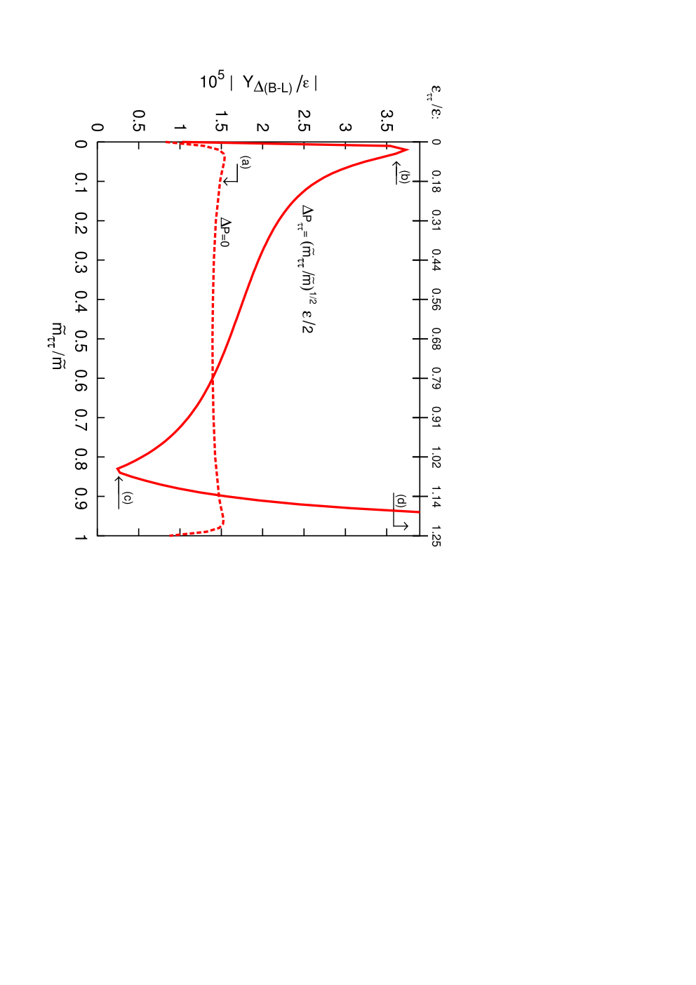
This qualitative expectation is confirmed by numerical integration of the flavour dependent Boltzmann equations. Fig. 9.2 (adapted from ref. [63]) depicts a set of possible cases. The absolute value of the final (in units of ) computed with GeV and eV is shown as a function of . Two flavour-aligned cases at (i.e. no component in ) and at (i.e. ) coincide with the results that would have been obtained by neglecting flavour. For quite different results are obtained. Case (dashed line) gives the results obtained by setting , that is by taking . As predicted in our qualitative analysis, the final asymmetry is practically independent of the flavour structure, and gets enhanced by a factor with respect to the flavour-aligned results.
For the more general cases where , the final doublet lepton asymmetry strongly depends on the particular flavour structure. To depict in a simple way the various possibilities, we adopt, as a convenient ansatz, the relation . This is based on the fact that, if we take the tree-level decay amplitude to zero () while keeping the total decay rate fixed [const.], vanishes as the square of this amplitude () while vanishes as the amplitude (). We extrapolate this proportionality to finite values of because this allows to represent the effects in a simple two-dimensional plot of versus .
On the upper -axis of Fig. 9.2 we mark for reference the relative value of the CP-asymmetry corresponding to the different values of . The most peculiar features are the two narrow regions marked with and where is strongly enhanced. In this happens around the ‘optimal’ value that yields a strong enhancement, even though is rather small. The region marked with corresponds to and to of the opposite sign with respect to . Here the steep rise of can reach values up to one order of magnitude larger than the vertical scale of the figure. (Note, however, that the ansatz does not yield the required behavior at the boundary and therefore the continuous line in the plot should not be extrapolated too close to this limit.) It is worth noticing that the two peaks correspond to values of of opposite sign. In fact, the asymmetry changes sign around point , and for it is of the opposite sign with respect to what one would obtain neglecting flavour effects. Similar results are expected in the temperature regime below GeV, when both the and the Yukawa reactions are in equilibrium. In this case even larger enhancements are possible because the dynamical production of the asymmetry of two flavours can occur in an ‘optimal’ regime.
In the weak washout regime for all the flavours, there can be no dynamical enhancement of the asymmetry and flavour effects are less important. The efficiencies for this regime are given in eqn (4.13) (or (9.12)). Using also eqn (9.7), we obtain
| (9.14) |
The first sum within square brackets is always so this contribution by itself is suppressed with respect to the unflavoured case. The second sum is always less than or equal to the largest of the ’s. Therefore, in this regime a necessary condition to have a large enhancement of the resulting doublet lepton asymmetry is that for at least one lepton flavour.
Finally, in the case where one flavour is weakly coupled to , , but other flavours are strongly coupled, , the singlet neutrinos are brought into equilibrium by the reactions involving the strongly coupled flavours, so that . The efficiency factor ‘loses’ the factor of , which corresponds to a suppressed abundance [see eq. (4.13)]. Consequently, the asymmetry for the weakly coupled flavour is given by
| (9.15) |
The asymmetry for the strongly coupled flavours is again given by eqn (9.13) with or 2.
9.3 Mixing of lepton flavour dynamics
In Section 6 we derive BE for the charge densities , without taking into account the SM spectator processes. For this reason, the dependence of the ’s on the ’s is left implicit. In Section 8 we analyze the spectator processes, assuming that decays to pure (flavour) states, that is, neglecting flavour effects. In this section we combine these two issues, and we outline how to express the washout term in eqn (6.56) in terms of the (see Appendix 14 for a more complete treatment).
We assume that asymmetries can be generated in two flavour directions, which we take to be and , where the latter is some linear combination of and . Below GeV, baryon and lepton numbers violating electroweak sphaleron processes, and -related processes are fast. In this situation, the charge densities that are (slowly) evolving because of the leptogenesis processes are
| (9.16) |
Note that, in the temperature range of interest, all the asymmetry-densities in the right-hand-side of this equation are generally non-vanishing. In particular, decays generate a non-vanishing chemical potential for the Higgs particles which, in turn (see eqn (14.5)), induces a non-vanishing chemical potential to the top-quarks. The QCD sphaleron condition of eqn (8.5) further implies that this happens for all the lighter quarks. The only exceptions are above GeV, and that is not populated during standard leptogenesis.
The asymmetry densities for the quarks and for the -singlet leptons can always be re-expressed in terms of the asymmetry densities of the -doublet leptons. This procedure makes use of the condition of hypercharge neutrality, eqn (14.4), that involves all three generation fermions. Consequently, once the appropriate substitutions are implemented, one obtains that the densities of the charges in eqn (9.16) correspond to linear combinations of the asymmetry densities of all the lepton doublets:
| (9.17) |
The matrix can then be inverted to give in terms of the charge densities (see Appendix 14). The same is true also for the Higgs asymmetry. We can thus write:
| (9.18) |
The matrix (introduced in ref. [65]) and the vector (introduced in ref. [204]) generalize the coefficients and , defined in eqn (8.4) for the case of pure flavour states, to the general flavour case. Their numerical values are determined by the relevant set of chemical equilibrium conditions, and therefore depend on temperature.

As a consequence of eqns (9.18), the evolution of one density depends on the other charge densities, that is, the BE for the lepton flavours form a system of coupled equations. This phenomenon is sometimes referred to as ‘electroweak sphaleron flavour mixing’, and was studied in refs. [63, 210]. One example of the possible effects is depicted in fig. 9.3. The plot gives the evolution of , and for the flavour configuration corresponding to the point labeled with in fig. 9.2. is in the strong washout regime, eV, and the CP asymmetry is relatively large, . For , the value eV is close to optimal, and the asymmetry is smaller in size and opposite in sign to : . For the relevant temperature, GeV, electroweak sphaleron, and reactions are in equilibrium, yielding the matrices of coefficients [in the basis]:
| (9.19) |
As apparent from fig. 9.3, gives the dominant contribution to the final asymmetry. A qualitative explanation goes as follows. For , a large asymmetry builds up quickly in the flavour and contributes to the early washout of (the sign of that is opposite to that of combines with the negative sign of yielding an increase of the washout rates). Thus, the early (negative) asymmetry in remains suppressed. It follows that the opposite sign asymmetry generated from decays at is largely unbalanced. As concerns the asymmetry, typically of strong washout regimes, it ‘freezes-out’ at with an absolute value that is sizably smaller than the values reached at earlier times.
Remarkably, as can be clearly seen in fig. 9.3, the asymmetry changes sign twice during its evolution. This peculiar behavior is qualitatively different from what would be obtained by neglecting the sphaleron induced flavour mixing, when there is a single change of sign. Other interesting washout effects induced by sphaleron mixing have been analyzed in ref. [211].
9.4 Phenomenological consequences
As discussed in Section 9.2, starting from a specific set of parameters within a given seesaw model, the inclusion of flavour effects in the calculation of the baryon asymmetry can change the result by factors of a few to orders of magnitude [63, 64]. In this section, we take a more “bottom-up” perspective of flavoured leptogenesis. As discussed below eqn (2.5), there are (currently) 14 unknown parameters in the three generation type I seesaw model, of which only a few are accessible to low energy experiments. It is interesting, from a phenomenological perspective, to constrain the unknown parameters by requiring that leptogenesis works successfully. We will find that the inclusion of flavour effects does not change the resulting constraints in a significant way.
9.4.1 The upper bound on the light neutrino mass scale
In the “single flavour” calculation, successful thermal leptogenesis requires a light mass scale eV [135, 212]. The argument leading to this bound does not apply in the flavoured calculation. Currently, there is no consensus in the literature on the value of the bound in the flavoured case. Analytic arguments (which we reproduce below) and the numerical analysis of Refs [62, 210, 180], suggest that flavoured leptogenesis can be tuned to work for up to eV. This is of the order of current bounds from Large Scale Structure data and WMAP [178, 179, 177, 119]. The leptogenesis bound is relaxed because there is more CP violation available in flavoured leptogenesis. The upper limit of eqn (5.17) on the total CP asymmetry decreases like , as the light neutrino mass scale increases. There is therefore an upper bound on ( for degenerate neutrinos). However, the limit (5.17) does not apply to the flavoured CP asymmetries, which can increase with the light neutrino mass scale, as shown in eqn (5.10).
The limit eV[135], obtained in the single flavour approximation, can be understood as follows. For such a high mass scale, the light neutrinos are almost degenerate, with . Due to the lower bound , leptogenesis takes place in the strong washout regime. Taking the total CP asymmetry to be close to the upper bound of eqn (5.17), the final baryon asymmetry can be approximated as
| (9.20) |
As the light neutrino mass scale is increased, and, correspondingly, the temperature of leptogenesis, must increase to compensate the suppression. The leptogenesis temperature is, however, bounded from above, by the requirement of having lepton number violating processes out of equilibrium. For instance, the requirement that the processes are out of equilibrium (we estimate , with from eqn 13.26) gives
| (9.21) |
which implies GeV. There is therefore an upper bound on the baryon asymmetry which scales as . A large enough baryon asymmetry is obtained for eV.
Consider now the flavoured case. We define and (with ), so that and . The individual flavour asymmetries, , satisfy the bound of eqn (5.10), while their sum satisfies the stricter bound of eqn (5.17). So, if we can arrange , then for strong flavoured washout, and for sufficiently slow processes, the final baryon asymmetry (from e.g. eqn (4.15)) is
| (9.22) |
To show that the eV bound does not apply in the flavoured case, we must demonstrate that the three ingredients that entered the derivation of eqn (9.22) – (i) an appropriate set of flavoured CP asymmetries, (ii) negligible processes, and (iii) strong flavoured washout – can be realized in a model.
(i) To obtain the desired decay rates and asymmetries we use the Casas-Ibarra [101] parametrization, in terms of , , and the complex orthogonal matrix (see the discussion around eqn (2.12)). This ensures that we obtain the correct low-energy parameters. We take for simplicity, and write as a rotation through the complex angle . The flavour asymmetries, for maximal atmospheric mixing, are
The flavour dependent decay rates and are proportional to
| (9.24) |
We see that we can choose and as required to obtain eqn (9.22) with .
(ii) Eqn (9.21) gives the condition for the processes to be out of equilibrium: GeV. Combined with eqn (9.22), this gives
| (9.25) |
(iii) In this strongly washed out area of parameter space, decays take place in the flavoured regime if [180, 181] (see Appendix 15.4). Suppose . Then eqn (9.22) is a valid estimate, provided when :
| (9.26) |
We conclude that with careful tuning, thermal leptogenesis can work for eV. This can be seen in Fig. 9.4. For the plot on the left, flavour effects are included, and leptogenesis can work for values . At the upper bound we have , so the cosmological bound is saturated.

9.4.2 Sensitivity of to low energy phases
An important, but disappointing, feature of “single-flavour” leptogenesis is the lack of a model-independent relation between CP violation in the leptogenesis processes and the (observable) phases of the lepton mixing matrix (see eqn (2.7)). With three singlet neutrinos , thermal leptogenesis can work with no CP violation in (see e.g. [213]) and, conversely, leptogenesis can fail in spite of non-vanishing phases in [214]. In some specific models, however, it is possible to establish a relation [215, 214].
In unflavoured leptogenesis, it is simple to see that the baryon asymmetry is insensitive to phases of [214]. Using the Casas-Ibarra parametrization of eqn (2.11) in eqn (5.13), can be written in a form where does not appear:
| (9.27) |
Alternatively, in the top-down parametrization in terms of , and (see Section 2.1.1), depends on the phases in , while the phases could arise only from .
The latter observation can be exploited to relate the phases to flavoured leptogenesis in models where there is no CP violation in 2222 22 Such models may be difficult to construct [216]. [63, 64, 217, 218, 219, 220]. However, for flavoured leptogenesis with three ’s, it is still true that the baryon asymmetry is not sensitive to phases of [221], in the sense that the baryon asymmetry can be accounted for with the phases of having any value. Conversely, if the phases of are measured, the baryon asymmetry is still not constrained. This can be seen from the scatter plots of ref. [221], which show that, for any value of the phases, the baryon asymmetry can be large enough.
In the two model (see section 2.1.2), there are three phases. Relations between phases and leptogenesis were obtained in unflavoured leptogenesis [106]. The relation between the flavoured CP asymmetries and the phases of , focusing on various texture models, was discussed in [222]. Possible relations between low energy observables and the baryon asymmetry, in the general case and for particular texture models, were discussed in [64].
9.4.3 The lower bound on
In the space of leptogenesis parameters, there is an envelope inside which leptogenesis can work. In the single-flavour calculation, the most important parameters are , (or, equivalently ), and the light neutrino mass scale [212]. Including flavour gives the parameter space more dimensions (…), but the envelope can still be projected onto the plane by fixing to its maximum value of eqn (5.17), which is a function of .
For thermal leptogenesis to take place, an adequate number density of must be produced by thermal scattering in the plasma, suggesting [59, 60]. There is a lower bound on , from requiring a large enough CP asymmetry. The corresponding bound on depends on the fine details of reheating, the dynamics of which has been studied in refs. [60, 59]. To avoid these complications, the lower bound on is usually quoted.
10 Variations
The bulk of this review focuses on thermal leptogenesis, with hierarchical singlet neutrinos, and where the CP asymmetry is generated in the decays of the lightest singlet neutrino. In this chapter, we give brief overviews of various alternative scenarios of leptogenesis. More detailed presentations can be found in the original literature, to which we give appropriate references.
10.1 Supersymmetric thermal leptogenesis
In the framework of supersymmetric seesaw models, new leptogenesis mechanisms become possible, such as Affleck-Dine leptogenesis or soft leptogenesis. In this subsection, we focus on the standard thermal leptogenesis scenario with hierarchical singlet ’s, where the presence of supersymmetry (SUSY) makes only small qualitative and quantitative differences [225, 54]. We have often referred to the supersymmetric modifications in previous chapters, so here we collect this information and summarize the differences that arise when calculating the baryon asymmetry in the supersymmetric type I seesaw.
Neglecting small SUSY-breaking terms, a singlet neutrino and its superpartner, the singlet sneutrino , have equal masses, equal decay rates and equal CP asymmetries . In this approximation, estimating the asymmetry in the minimal supersymmetric standard model (MSSM) with respect to the SM case (at fixed values of the Yukawa couplings and masses) amounts to a (careful) counting of a few numerical factors:
- 1.
There are twice the number of states running in the loops, and thus the CP asymmetries and are roughly twice the SM value of (see the loop function in eqn (5.15)).
- 2.
Including the asymmetry generated in decays gives another enhancement of a factor of two.
- 3.
In the MSSM, the plasma is populated by twice as many particles as there are in the SM. More precisely, we have . Thus the lepton asymmetries to entropy ratios are reduced by .
- 4.
Due to the additional final states, the decay rate is twice faster than in the SM. (For the scalar neutrinos there are also two channels .) In the strong washout regime, the associated inverse-decay reactions double the washout rates, reducing the asymmetry by a factor of two. In the weak washout regime, the production of and is more efficient, and this increases the asymmetry by the same factor.
- 5.
The expansion rate of the Universe is proportional to and is therefore roughly a factor of faster in SUSY (). This reduces the time during which the strong washout processes can erase the asymmetry, yielding a enhancement. For weak washouts, it reduces the time for and production, yielding a suppression of the final asymmetry.
- 6.
Putting all these factors together, we estimate:
| (10.1) |
Thus, in the MSSM, in spite of the doubling of the particle spectrum and of the large number of new processes involving superpartners [186], one does not expect major numerical changes with respect to the non-supersymmetric case.
Supersymmetric thermal leptogenesis has a potential gravitino problem [76, 77, 79, 80]. After inflation, the universe thermalizes to a reheat temperature . Gravitinos are produced by thermal scattering in the bath, and the rate is higher at higher temperatures. The gravitinos are long-lived; if there are lighter SUSY particles (the gravitino is not the LSP), the decay rate can be estimated as [79]
| (10.2) |
If too many gravitinos decay during or after Big Bang Nucleosynthesis (at seconds), the resulting energetic showers in the thermal bath destroy the agreement between predicted and observed light element abundances[75, 78, 81]. There are several possible solutions to the gravitino problem:
As discussed in Section 5.2, there is a lower bound on the reheat temperature GeV, to produce a big enough baryon asymmetry by thermal leptogenesis (in the three generation type I seesaw with hierarchical masses). This is difficult to reconcile with the first solution described above [231], which is arguably the most plausible one in gravity mediated scenarios. A large enough baryon asymmetry can be produced at lower , if , the decay width.
10.2 Less hierarchical ’s
It is crucial for thermal leptogenesis that there are more than one singlet neutrino. In particular, the CP asymmetry that is produced in decays comes from interference between the tree diagram and the loop diagrams involving the heavier as virtual particles in the loop. In the conventional picture, however, one assumes a strong hierarchy, . Then, an upper bound on the CP asymmetry in decays applies (see eqn (5.10)),which provides much of the predictive power of the conventional leptogenesis scenario.
However, as mentioned in section 5.2, when the singlet neutrino masses are not very strongly hierarchical, a term that is higher order in can become important. Specifically, there is a contribution to the CP asymmetry that is proportional to and does not vanish when the light neutrino masses are degenerate [162, 163].
In addition to this effect of the heavier singlet neutrino masses on the CP asymmetry in the decays, there are also interesting effects related to the decays of the heavier singlet neutrinos themselves. These effects are discussed in the following subsection.
10.2.1 effects
When analyzing leptogenesis, the effects of and are often neglected. This is reasonable if . However, if , one should not assume that the -violating interactions of would washout any lepton asymmetry generated at temperatures and, in particular, the asymmetry generated in the decays of . Under various (rather generic) circumstances, the lepton asymmetry generated in decays survives the leptogenesis phase. Thus, it is quite possible that the lepton asymmetry relevant for baryogenesis originates mainly (or, at least, in a non-negligible part) from decays.
The possibility that leptogenesis can successfully explain the baryon asymmetry of the Universe has been shown in two limiting cases:
- 1.
- 2.
It is plausible that the role of leptogenesis cannot be ignored also in the intermediate range for couplings, but the analysis in this case is complicated and has not been carried out yet.
The -decoupling scenario is simple to understand. It applies when is weakly coupled to the lepton doublets (see eqn (4.7):
| (10.3) |
where and
| (10.4) |
In this case, the asymmetry generated in thermal leptogenesis is too small. Furthermore, the washout effects are negligible and, consequently, the asymmetry generated in decays survives.
We next discuss leptogenesis in the strong -coupling limit. We are interested in the case that a sizeable asymmetry is generated in decays, while leptogenesis is inefficient. We thus assume that the -related washout is not too strong, while the -related washout is so strong that it makes leptogenesis fail:
| (10.5) |
To further simplify the analysis, we impose two additional conditions [188]: thermal leptogenesis, and strong hierarchy, . These two conditions together guarantee that
| (10.6) |
Thus, the dynamics of and are decoupled: there are neither -related washout effects during leptogenesis, nor -related washout effects during leptogenesis.
The decays into a combination of lepton doublets that we denote by :
| (10.7) |
The second condition in (10.5) implies that already at the -Yukawa interactions are sufficiently fast to quickly destroy the coherence of . Then a statistical mixture of and of the state orthogonal to builds up, and it can be described by a suitable diagonal density matrix. On general grounds, one expects that decoherence effects proceed faster than washout. In the relevant range, , this is also ensured by the fact that the dominant washout process (the inverse decay ) is blocked by thermal effects [60], and only scatterings with top-quarks and gauge bosons, that have additional suppression factors of and , contribute to the washout.
Let us consider the case where both and decay at GeV, so that flavour effects are irrelevant. We also neglect the effects of interactions, which are generically in equilibrium at few GeV. (This scenario is interesting to consider, even though it may only occur in a narrow temperature range.) A convenient choice for an orthogonal basis for the lepton doublets is where, without loss of generality, satisfies . Then the asymmetry produced in decays decomposes into two components:
| (10.8) |
where and . The crucial point here is that we expect, in general, and, since , is protected against washout. Consequently, a finite part of the asymmetry from decays survives through leptogenesis. A more detailed analysis [188] finds that is not entirely washed out, and that the final lepton asymmetry is given by .
For , flavour issues modify the quantitative details, but the qualitative picture, and in particular the survival of a finite part of , still hold. On the other hand, for , the full flavour basis is resolved and, in general, there are no directions in flavour space where an asymmetry is protected and can be erased entirely.
The conclusion is that and leptogenesis cannot be ignored, unless at least one of the following conditions applies:
- 1.
The asymmetries and/or the washout factors vanish, and .
- 2.
-related washout is still significant at .
- 3.
The reheat temperature is below .
In all other cases, the -related parameters play a role in determining the baryon asymmetry of the Universe. Consequently, relations between these parameters and neutrino masses are important. Such relations were obtained in Ref. [106, 136], and they lead, for the case that the light neutrino masses have normal hierarchy, to the following consequences:
- •
In the framework with two singlet neutrinos, both and interactions are in the strong washout regime, with both eV [106], and at least one eV.
- •
In the framework with three singlet neutrinos, at least two ’s have interactions in the strong washout regime, with eV and at least one eV.
The lower bounds are stronger for inverted hierarchy, and even more so in the framework with three singlet neutrinos and quasi-degenerate light neutrinos.
10.2.2 Resonant leptogenesis
A resonant enhancement of the CP asymmetry in decay occurs when the mass difference between and is of the order of the decay widths. Such a scenario has been termed ‘resonant leptogenesis’, and has benefited from many studies in different formalisms 2323 23 See [233] for a comparison of the different calculations. [82, 234, 235, 85, 236, 189, 237, 238, 61, 184, 239, 240, 131, 132, 241, 242, 243, 244]. As this review focuses on hierarchical , we briefly list the idea and some references.
The resonant effect is related to the self energy contribution to the CP asymmetry. Consider, for simplicity, the case where only is quasi-degenerate with . Then, the self-energy contribution involving the intermediate , to the total CP asymmetry (we neglect important flavour effects [61]) is given by
| (10.9) |
The resonance condition reads
| (10.10) |
In this case
| (10.11) |
Thus, in the resonant case, the asymmetry is suppressed by neither the smallness of the light neutrino masses, nor the smallness of their mass splitting, nor small ratios between the singlet neutrino masses. Actually, the CP asymmetry could be of order one. (More accurately, .)
With resonant leptogenesis, the Boltzmann Equations are different. The densities of and are followed, since the both contribute to the asymmetry, and the relevant timescales are different. For instance, the typical time-scale to build up coherently the CP asymmetry is unusually long, of order . In particular, it can be larger than the time-scale for the change of the abundance of the sterile neutrinos. This situation implies that quantum effects in the Boltzmann equations can be significant, in the weak or mild washout regime, for resonant leptogenesis [241, 242].
The fact that the asymmetry could be large, independently of the singlet neutrino masses, opens up the possibility of low scale resonant leptogenesis. Models along these lines have been constructed in Refs. [236, 61, 240, 245]. It is a theoretical challenge to construct models where a mass splitting as small as the decay width is naturally achieved. For attempts that utilize approximate flavour symmetries see, for example, [189, 237, 239, 243, 246], while studies of this issue in the framework of minimal flavour violation can be found in [131, 132, 244].
10.3 Soft leptogenesis
The modifications to standard leptogenesis due to supersymmetry have been discussed in section 10.1. The important parameters there are the Yukawa couplings and the singlet neutrino parameters, which are all superpotential terms (see eqn 2.21):
| (10.12) |
Supersymmetry must, however, be broken. In the framework of the supersymmetric standard model extended to include singlet neutrinos (SSM+N), there are, in addition to the soft supersymmetry breaking terms of the SSM, terms that involve the singlet sneutrinos , in particular bilinear () and trilinear () scalar couplings. These terms provide additional sources of lepton number violation and of CP violation. Scenarios where these terms play a dominant role in leptogenesis have been termed ‘soft leptogenesis’ [86, 87, 247, 248, 249, 250, 251, 252, 253, 254, 255, 256, 257, 258].
Soft leptogenesis would have taken place even with a single lepton generation. To simplify things we work, therefore, in the framework of a single generation SSM+N. The relevant soft supersymmetry terms in the Lagrangian are given in eqn (10.13):
| (10.13) |
In addition, the electroweak gaugino masses play a role:
| (10.14) |
Here () are the gauginos. The effects related to , the gaugino, are similar to (and usually less important than) those of , so we do not present them explicitly.
The Lagrangian derived from eqns (10.12), (10.13) and (10.14) has two independent physical CP violating phases:
| (10.15) | |||||
| (10.16) |
These phases give the CP violation that is necessary to dynamically generate a lepton asymmetry. If we set the lepton number of and to , so that (and ) are lepton number conserving, then (and ) violate lepton number by two units. Thus processes that involve and give the lepton number violation that is necessary for leptogenesis.
A crucial role in soft leptogenesis is played by the mixing amplitude,
| (10.17) |
( is the dispersive part of the mixing amplitude, while is the absorptive part), which induces mass and width differences,
| (10.18) |
( is the average width) between the two mass eigenstates, the heavy , and the light ,
| (10.19) |
The ratio depends on the mixing amplitude ratio:
| (10.20) |
Also of importance are the decay amplitudes of or into various final states :
| (10.21) |
The decay width of the singlet sneutrino is given by (for )
| (10.22) |
while the mixing parameters are given by
| (10.23) | |||||
The quantity of interest is the CP asymmetry in singlet sneutrino decay,
| (10.24) |
where is the time-integrated decay rate into a final state with leptonic content . Here is the (anti)lepton doublet and is the (anti)slepton doublet.
Qualitatively, the most special feature of soft leptogenesis is that it gets contributions that are related to CP violation in mixing. This is a phenomenon that is analogous to the CP violation in mixing, where it leads to the decays, the process where CP violation was first discovered. A relative CP violating phase between and of eqn (10.17) gives [see eqn (10.19)] which, in turn, leads to a situation where the mass eigenstates are not CP eigenstates. One such contribution is given by [86, 87]
| (10.25) |
Here is the scale of the soft supersymmetry breaking terms ( and ), and
| (10.26) |
where () are phase space factors for final states involving scalars (fermions). At zero temperature, , but for temperature at the time of decay that is comparable to the singlet neutrino mass we have . The difference between and at finite temperature arises from the Pauli blocking of final state fermions and Bose-Einstein stimulation of decays into scalars.
The contribution (10.25) stands out among the soft leptogenesis contributions as the only one that is linear in the ratio . (All other contributions are quadratic in this ratio.) Thus, for , this is the only contribution that is potentially significant. Indeed, it could account for the observed baryon asymmetry if the following conditions are all fulfilled:
- 1.
The lightest singlet sneutrino is light enough, GeV.
- 2.
The Yukawa couplings are small enough, . The lighter is , the smaller the Yukawa coupling must be.
- 3.
The parameter is well below its naive value, . The lighter is , the more suppressed must be.
For , there are several other contributions that can be significant [86]. All of these contributions involve and are therefore proportional to the weak coupling . In addition, as mentioned above, they are proportional to . In particular, there are contributions related to CP violation in decay (a phenomenon that is analogous to the one giving in decays and to the vertex contribution in standard leptogenesis), and to CP violation in the interference of decays with and without mixing (analogous to in decays). These two contributions are suppressed by but no other small factors. In particular, unlike the contribution of eqn (10.25), these contributions do not vanish when and therefore they allow .
Soft leptogenesis is an interesting scenario in the framework of the supersymmetric seesaw for several reasons. First, the relevant new sources of CP violation and lepton number violation appear generically in this framework. In this sense, soft leptogenesis is qualitatively unavoidable in the SSM+N framework, and the question of its relevance is a quantitative one. Second, if GeV (in the supersymmetric framework, this range is preferred by the gravitino problem), then standard leptogenesis encounters problems, while soft leptogenesis can be significant. Third, if , then it is almost unavoidable that soft leptogenesis plays an important role.
10.4 Dirac leptogenesis
The extension of the Standard Model with singlet neutrinos allows two different ways of giving the active neutrinos their very light masses. First, one can invoke the seesaw mechanism which gives Majorana masses to the light neutrinos. This extension has at least three attractive features:
- •
No extra symmetries (and, in particular, no global symmetries) have to be imposed.
- •
The extreme lightness of neutrino masses is linked to the existence of a high scale of new physics, which is well motivated for various other reasons (e.g. gauge unification).
- •
Lepton number is violated, which opens the way for leptogenesis.
The second way is to impose lepton number and give Dirac masses to the neutrinos. A-priori, one might think that all three attractive features of the seesaw mechanism are lost. Indeed, one must usually impose additional symmetries. But one can still construct natural models where the tiny Yukawa couplings that are necessary for small Dirac masses are related to a small breaking of a symmetry. What is perhaps most surprising is the fact that leptogenesis could proceed successfully even if the neutrinos are Dirac particles and lepton number is not broken [259, 260] (except, of course, by the sphaleron interactions). Such scenarios have been termed ‘Dirac leptogenesis’ [260, 261, 262, 263, 264, 265, 266]. Actually, the success of Dirac leptogenesis is closely related to the extreme smallness of the neutrino Yukawa couplings in this scenario.
An implementation of the idea is the following. A CP violating decay of a heavy particle can result in a non-zero lepton number for left-handed particles, and an equal and opposite non-zero lepton number for right-handed particles, so that the total lepton number is zero. For the charged fermions of the Standard Model, the Yukawa interactions are fast enough that they quickly equilibrate the left-handed and the right-handed particles, and the lepton number stored in each chirality goes to zero. This is not true, however, for Dirac neutrinos. The size of their Yukawa couplings is , which means that equilibrium between the lepton numbers stored in left-handed and right-handed neutrinos will not be reached until temperatures fall well below the electroweak breaking scale. To see this, note that the rate of the Yukawa interactions is given by . It becomes significant when it equals the expansion rate of the Universe, . Thus, the temperature of equilibration between left-handed and right-handed neutrinos can be estimated as . By this time, the left-handed lepton number has been partially transformed into a net baryon number by the sphaleron interactions.
More specifically, consider a situation where the CP violating decays of some new, heavy particles have produced a negative lepton number in left-handed neutrinos, and a positive lepton number, of equal magnitude, in right-handed neutrinos. The sphalerons interact with the left-handed neutrinos, violating and conserving . Consequently, part of the negative lepton number stored in the left-handed neutrinos is converted to a positive baryon number. At much lower temperatures, when sphaleron interactions (and and violation) are frozen, the remaining negative lepton number in left-handed neutrinos equilibrates with the positive lepton number stored in the right handed-neutrinos. Since, however, the negative lepton number in left-handed neutrinos has become smaller in magnitude than the positive lepton number in right-handed neutrinos, a net lepton number remains. The final situation is then a Universe with total positive baryon number, total positive lepton number, and .
A specific example of a natural, supersymmetric model with Dirac neutrinos is presented in Ref. [261]. The Majorana masses of the -superfields are forbidden by (lepton number symmetry). The neutrino Yukawa couplings are forbidden by a symmetry where, among all the SSM+N fields, only the superfields are charged. The symmetry is spontaneously broken by the vacuum expectation value of a scalar field that can naturally be at the weak scale, . This breaking is communicated to the SSM+N via extra, vector-like lepton doublet fields, , that have masses much larger than . Consequently, the neutrino Yukawa couplings are suppressed by the small ratio . The CP violation arises in the decays of the vector-like leptons, whereby and . The resulting asymmetries in and in are equal in magnitude and opposite in sign.
The main phenomenological implications of Dirac leptogenesis is the absence of any signal in neutrinoless double beta decays.
10.5 Triplet scalar leptogenesis
As explained in Subsection 2.2, one can generate see-saw masses for the light neutrinos by tree-level exchange of -triplet scalars. Since this mechanism necessarily involves lepton number violation, and allows for new CP violating phases, it is interesting to examine it as a possible source of leptogenesis [267, 268, 111, 269, 270, 249, 271, 272, 273, 254, 274, 275, 276, 277, 278, 279, 280, 281]. One obvious problem in this scenario is that, unlike singlet fermions, the triplet scalars have gauge interactions that keep them close to thermal equilibrium at temperatures GeV. It turns out, however, that successful leptogenesis is possible even at a much lower temperature. This subsection is based in large part on Ref. [274], where further details and, in particular, an explicit presentation of the relevant Boltzmann equations can be found.
The CP asymmetry that is induced by the triplet scalar decays is defined as follows:
| (10.27) |
The overall factor of 2 comes because the triplet scalar decay produces two (anti)leptons.
To calculate , one should use the Lagrangian terms given in eqn (2.15). While a single triplet is enough to produce three light massive neutrinos, there is a problem in leptogenesis if indeed this is the only source of neutrinos masses: The asymmetry is generated only at higher loops and in unacceptably small.
It is still possible to produce the required lepton asymmetry from a single triplet scalar decays if there are additional sources for the neutrino masses, such as type I, type III, or type II contributions from additional triplet scalars. Define () as the part of the light neutrino mass matrix that comes (does not come) from the contributions of the triplet scalar that gives :
| (10.28) |
Then, assuming that the particles that are exchanged to produce are all heavier than , the CP asymmetry is given by
| (10.29) |
where ( is the tree-level branching ratio to leptons (Higgs doublets). If these are the only decay modes, i.e. , then . There is an upper bound on this asymmetry:
| (10.30) |
Note that, unlike the singlet fermion case, increases with larger .
As concerns the efficiency factor, it can be close to maximal, , in spite of the fact that the gauge interactions tend to maintain the triplet abundance very close to thermal equilibrium. There are two necessary conditions that have to be fulfilled by the two decay rates, and , in order that this will happen [274]:
- 1.
One of the two decay rates is faster than the annihilation rate.
- 2.
The other decay mode is slower than the expansion rate of the Universe.
The first condition guarantees that gauge scatterings are ineffective: the triplets decay before annihilating. The second condition guarantees that the fast decays do not lead to a strong washout of the lepton asymmetry: lepton number is violated only by the simultaneous presence of and .
Combining a calculation of and the upper bound on the CP asymmetry (10.30), successful leptogenesis implies a lower bound on the triplet mass varying between GeV and GeV, depending on the relative weight of and in the light neutrino mass.
10.6 Triplet fermion leptogenesis
As explained in Subsection 2.3, one can generate see-saw masses for the light neutrinos by tree-level exchange of -triplet fermions. This mechanism necessarily involves lepton number violation, and allows for new CP violating phases so we should examine it as a possible source of leptogenesis [282, 162, 270]. This subsection is based in large part on Ref. [270], where further details and, in particular, an explicit presentation of the relevant Boltzmann equations can be found.
As concerns neutrino masses, the formalism and qualitative features are very similar to the singlet fermion case. As concerns leptogenesis, there are, however, qualitative and quantitative differences.
With regard to the CP asymmetry from the lightest triplet fermion decay, the relative sign between the vertex loop contribution and the self-energy loop contribution is opposite to that of the singlet fermion case. Consequently, in the limit of strong hierarchy in the heavy fermion masses, the asymmetry in triplet decay is 3 times smaller than in the singlet decay (see the discussion in Section 5.2 for the singlet case and for definitions). On the other hand, since the triplet has three components, the ratio between the final baryon asymmetry and is 3 times bigger. The decay rate of the heavy fermion is the same in both cases. This, however, means that the thermally averaged decay rate is 3 times bigger for the triplet, as is the on-shell part of the scattering rate.
A significant qualitative difference arises from the fact that the triplet has gauge interactions. The effect on the washout factor is particularly significant for eV, the so-called “weak washout regime” (note that this name is inappropriate for triplet fermions). The gauge interactions still drive the triplet abundance close to thermal equilibrium. A relic fraction of the triplet fermions survives. The decays of these relic triplets produce a baryon asymmetry, with
| (10.31) |
The strong dependence on is a result of the fact that the expansion rate of the Universe is slower at lower temperatures. On the other hand, for eV, the Yukawa interactions are responsible for keeping the heavy fermion abundance close to thermal equilibrium, so the difference in between the singlet and triplet case is only .
Ignoring flavour effects, and assuming strong hierarchy between the heavy fermions, Ref. [270] obtained a lower bound on the mass of the lightest heavy triplet fermion:
| (10.32) |
When the triplet fermion scenario is incorporated in a supersymmetric framework, and the soft breaking terms do not play a significant role, the modifications to the above analysis is by factors of .
11 Conclusions
During the last few decades, a large set of experiments involving solar, atmospheric, reactor and accelerator neutrinos have converged to establish that the standard model neutrinos are massive. The seesaw mechanism extends the standard model in a way that allows neutrino masses. It provides a nice explanation of the suppression of the neutrino masses with respect to the electroweak breaking scale, which is the mass scale of all standard model charged fermions. Furthermore, without any addition or modification, it can also account for the observed baryon asymmetry of the Universe. The possibility of giving an explanation of two apparently unrelated experimental facts – neutrino masses and the baryon asymmetry – within a single framework that is a natural extension of the standard model, together with the remarkable ‘coincidence’ that the same neutrino mass scale suggested by neutrino oscillation data is also optimal for leptogenesis, makes the idea that baryogenesis occurs through leptogenesis a very attractive one.
Leptogenesis can be quantitatively successful without any fine-tuning of the seesaw parameters. Yet, in the non-supersymmetric seesaw framework, a fine-tuning problem arises due to the large corrections to the mass-squared parameter of the Higgs potential that are proportional to the heavy Majorana neutrino masses (see Section 2.4). Supersymmetry can cure this problem, avoiding the necessity of fine tuning. However, the gravitino problem that arises in many supersymmetric models requires a low reheat temperature after inflation, in conflict with generic leptogenesis models (see Section 10.1). Thus, constructing a fully satisfactory theoretical framework that implements leptogenesis within the seesaw framework is not a straightforward task.
From the experimental side, the obvious question to ask is if it is possible to test whether the baryon asymmetry has been really produced through leptogenesis. Unfortunately it seems impossible that any direct test can be performed. To establish leptogenesis experimentally, we need to produce the heavy Majorana neutrinos and measure the CP asymmetry in their decays. However, in the most natural seesaw scenarios, these states are simply too heavy to be produced, while if they are light, then their Yukawa couplings must be very tiny, again preventing any chance of direct measurements.
The possibility of indirect tests from measurements of the asymmetries produced by leptogenesis is also ruled out. This is because there are too many high energy parameters that are relevant to leptogenesis and, even if we adopt the most optimistic point of view, there are at most four observables. These are the value of the baryon asymmetry that is known with a good accuracy (see Section 1.1), and the three cosmic neutrino flavour asymmetries that we do not know how to measure. A measurement of the total lepton asymmetry would be very valuable. If a value of the order of the baryon asymmetry were found, it would provide strong evidence that electroweak sphalerons have been at work in the early Universe.2424 24 The opposite result would not disprove sphaleron physics: see [283, 284] for a model in which production of a large lepton asymmetry after sphalerons freeze-out can yield orders of magnitude larger than . Even if we have no reason to doubt that sphaleron processes occurred in the thermal bath with in-equilibrium rates, they are the fundamental ingredient of the whole leptogenesis idea, and thus the importance of an experimental test should not be underappreciated. Measurements of the single lepton flavour asymmetries would provide some information on leptogenesis parameters (on the flavour CP asymmetries if leptogenesis occurred in the unflavoured regime, or on a combination of the flavour CP asymmetries and of the flavour-dependent washouts otherwise). However, at present, we have not even observed the relic neutrino background, and the possibility of revealing asymmetries in this background seems completely hopeless.
Lacking the possibility of a direct proof, experiments can still provide circumstantial evidence in support of leptogenesis by establishing that (some of) the Sakharov conditions for leptogenesis (see Section 1.2) are realized in nature.
Planned neutrinoless double beta decay () experiments (GERDA [285], MAJORANA [286], CUORE [287]) aim at a sensitivity to the effective neutrino mass in the few 10 meV range. If they succeed in establishing the Majorana nature of the light neutrinos,2525 25 This is likely to happen if neutrinos are quasi-degenerate or if the mass hierarchy is inverted this will strengthen our confidence that the seesaw mechanism is at the origin of the neutrino masses and, most importantly, will establish that the first Sakharov condition for the dynamical generation of a lepton asymmetry, that is that lepton number is violated in nature, is satisfied.
Proposed SuperBeam facilities [288, 289] and second generation off-axis SuperBeams experiments (T2HK [290], NOA [291]) can discover CP violation in the leptonic sector. These experiments can only probe the Dirac phase of the neutrino mixing matrix. They cannot probe the Majorana low energy or the high energy phases, but the important point is that they can establish that the second Sakharov condition for the dynamical generation of a lepton asymmetry is satisfied.2626 26 As discussed in [292], it is conceivable (but not natural) that the Dirac phase is solely responsible for the matter-antimatter asymmetry.
In contrast to the previous two conditions, verifying that the decays of the heavy neutrinos occurred out of thermal equilibrium (the third condition) remains out of experimental reach, since it would require measuring the heavy neutrino masses and the size of their couplings.
Given that we do not know how to prove that leptogenesis is the correct theory, we might ask if there is any chance to falsify it. Indeed, future neutrino experiments could weaken the case for leptogenesis, or even falsify it, in two main ways: Establishing that the seesaw mechanism is not responsible for the observed neutrino masses, or finding evidence that the washout is too strong.
By itself, failure in revealing signals of decays will not disprove leptogenesis. Indeed, with normal neutrino mass hierarchy one expects that the rates of lepton number violating processes are below experimental sensitivity. However, if neutrinos masses are quasi-degenerate or inversely hierarchical, and future measurements of the oscillation parameters will not fluctuate too much away from the present best fit values, the most sensitive decay experiments scheduled for the near future should be able to detect a signal [72].2727 27 decay experiments are sensitive to the effective mass parameter . In the inverted hierarchy scenario the contribution to can be neglected, and approximating for simplicity one gets . Since deviates from maximal mixing, we can then predict that should be of the order of the atmospheric mass scale, independently of the values of the Majorana phases and . If instead the limit on is pushed below meV (a quite challenging task), this would suggest that either the mass hierarchy is normal, or neutrinos are not Majorana particles. The latter possibility would disprove the seesaw model and standard leptogenesis (see however section 10.4). Thus, determining the order of the neutrino mass spectrum is extremely important to shed light on the connection between decay experiments and leptogenesis.
Long baseline neutrino experiments can achieve this result [293, 294] by exploiting the fact that oscillations in matter can determine the sign of the atmospheric mass difference . In fact, if the oscillations of atmospheric neutrinos involve the heaviest (lightest) state, corresponding to normal (inverted) hierarchy, then oscillations are enhanced (suppressed) while , oscillations are suppressed (enhanced).
Cosmology could also provide important information in establishing if the neutrino mass hierarchy is inverted. Cosmological observations are sensitive to the sum of the three neutrino masses . In the near future, improved CMB data and more precise large scale structure measurements can push the sensitivity on down to the eV level. For an inverted hierarchy a signal should be detected around or above this value.
In summary, if it is established that the neutrino mass hierarchy is inverted and at the same time no signal of decays is detected at a level meV, one could conclude that the seesaw is not at the origin of the neutrino masses, and that leptogenesis is not the correct explanation of the baryon asymmetry.
The neutrino mass scale has also more direct implications for leptogenesis. A quantitatively successful leptogenesis prefers a mass scale for the light neutrinos not larger than a few times the atmospheric neutrino mass scale (see Section 9.4.1). In particular, in the standard type I seesaw model (see section 2.1), if leptogenesis occurs in the unflavoured regime and the heavy Majorana neutrinos are sufficiently hierarchical, leptogenesis would fail to produce enough baryon asymmetry when the neutrino mass scale exceeds values as low as eV. Indeed, if past experiments had detected neutrino masses of order a few eV, leptogenesis, if not completely ruled out, would have certainly lost most of its theoretical appeal. In the future, a discovery of a neutrino mass at the decay experiment KATRIN will also put the type I seesaw scenario for leptogenesis in serious doubt, since it will yield a mass value a bit too large (the claimed discovery potential is for an effective -decay mass parameter of about 0.35 eV [295]). However, cosmological observations have already reached a sensitivity to somewhat below eV [296, 297, 298], implying that it is unlikely that leptogenesis could be put to doubt by a direct detection of neutrino masses in laboratory experiments.
As concerns CP violation, a failure in detecting leptonic CP violation will not weaken the case for leptogenesis in a significant way. Instead, it would mean that the Dirac CP phase (or the mixing angle, or both) is small enough to render CP violating effects unobservable.
Finally, the CERN LHC has the capability of providing information that is relevant to leptogenesis. First, electroweak baryogenesis (see Section 1.2) can be tested at the LHC. It will become strongly disfavored (if not completely ruled out) if supersymmetry is not found, or if supersymmetry is discovered but the stop and/or the Higgs are too heavy. Eliminating various scenarios that are able to explain the baryon asymmetry will strengthen the case for the remaining viable possibilities, including leptogenesis. Conversely, if electroweak baryogenesis is established by the LHC (and EDM) experiments, the case for leptogenesis will become weaker.
Second, new physics discoveries at the LHC can play a fundamental role in establishing that the origin of the neutrino masses is not due to the seesaw mechanism, leaving no strong motivation for leptogenesis. This may happen in several different ways. For example (assuming that the related new physics is discovered), the LHC will be able to test if the detailed phenomenology of any of the following models is compatible with an explanation of the observed pattern of neutrino masses and mixing angles: supersymmetric R-parity violating couplings and/or L-violating bilinear terms [299, 300]; leptoquarks [301, 302]; triplet Higgses [303, 304]; new scalar particles of the type predicted in the Zee-Babu [305, 306] types of models [307, 308, 309]. It is conceivable that such discoveries can eventually exclude the seesaw mechanism and rule out leptogenesis.
To conclude, the seesaw framework provides the most natural and straightforward explanation of the light neutrino masses and has, in principle, all the ingredients that are necessary for successful leptogenesis. This makes leptogenesis arguably the most attractive explanation for the observed baryon asymmetry. This scenario has limited predictive power for low energy observables, so it is unlikely to be directly tested. Yet, future experiments have the potential of strengthening, or weakening, or even falsifying the case for leptogenesis.
Acknowledgements
This review is based on collaborations with many people over many years, and parts of it are copied from the resulting papers. We thank our various collaborators for the pleasure of working with them, and for their assistance in writing this review.
SD is grateful to many people for useful discussions, and comments on the manuscript; in particular E Akhmedov, G Branco, L Covi, P Di Bari, J Garayoa, GF Giudice, F Joaquim, FX Josse-Michaux, M Laine, S Lavignac, M Losada, S Petkov, G Raffelt, G Rebelo, V Rubakov and A Santamaria. SD would like to thank all her leptogenesis collaborators: A Abada, L Boubekeur, B Campbell, J Garayoa, A Ibarra,R Kitano, M Losada, F-X Josse-Michaux, K Olive, F Palorini, M Peloso, A Riotto, L Sorbo and N Rius, for productive collaborations. And as usual, a special thanks to A Strumia for comments, discussions and contributions. The collaboration of SD with M Losada and A Abada was partially supported by ECOS.
EN acknowledges fruitful collaborations in leptogenesis with Diego Aristizabal, Guy Engelhard, Yuval Grossman, Marta Losada, Luis Alfredo Muñoz, Jorge Noreña, Juan Racker and Esteban Roulet. The work of EN is supported in part by Colciencias in Colombia under contract 1115-333-18739.
YN thanks his leptogenesis collaborators: Guy Engelhard, Yuval Grossman, Tamar Kashti, Juan Racker and Esteban Roulet. The research of YN is supported by the Israel Science Foundation (ISF), by the United States-Israel Binational Science Foundation (BSF), by the German-Israeli Foundation for Scientific Research and Development (GIF), and by the Minerva Foundation.
12 Appendix: Notation
| dimensionless time variable | 13.10 | |
| 6.10 | ||
| Hubble rate, Hubble rate at | 13.7, 13.11 | |
| entropy density | 13.6 | |
| ratio of number density to entropy density | 13.6 | |
| number density for particle in kinetic equilibrium | 13.2, 13.5 | |
| in kinetic equilibrium | 6.3, 13.6 | |
| ratio of and density to entropy density ( | after 6.3 | |
| density of doublets and singlets of flavour | 6.7 | |
| 6.3 | ||
| 6.3 | ||
| ratio of asymmetry to entropy density | 6.9, 14.11 | |
| ratio of baryon asymmetry to entropy density | 1.2, 4.1, 16.10 | |
| degrees of freedom in the thermal bath | 13.8, 13.9 | |
| internal degrees of freedom of particle | below 13.3 | |
| efficiency parameter for flavour | 4.1, 16.7, 16.8 | |
| CP asymmetry in flavour | 5.1, 5.13 | |
| light neutrino mass matrix | 2.2 | |
| largest, smallest light neutrino mass | 5.10, 5.17 | |
| (rescaled) decay rates, Hubble expansion rate | 4.7 | |
| matrix relating the to the | 14.14 14.15 | |
| neutrino Yukawa coupling | 2.3 | |
| Yukawa coupling of particle (not a neutrino) | 2.3 | |
| Higgs vev (GeV) | 2.3 | |
| total decay rate | 4.4, 13.20 | |
| total inverse decay rate | 4.10 | |
| partial decay rate to flavour and antiflavour : | 4.10 | |
| branching ratio | 5.10 | |
| rate density for | 13.14 | |
| rate density for two body decays of | 13.21 | |
| rate, rate density of Yukawa interaction | 14.10 | |
| CP difference: | 6.2 | |
| difference between process and its time reversed | 6.4 | |
| with exchange of on-shell particle removed | 6.5 | |
| Bessel functions | 13.19, 13.3 | |
| matrix element, amplitude | 5.2 | |
| 4-momentum conservation: | 5.6 | |
| phase space | 5.6 |
13 Appendix: Kinetic Equilibrium
The interested reader can find a more complete set of formulae for example in the Appendices of refs. [31, 310].
13.1 Number densities
Of the particles relevant to leptogenesis, all but the ’s carry charges under the standard model gauge group and are, therefore, subject to gauge interactions. We take the distributions of the (non-singlet) particle species to have their kinetic equilibrium form, because gauge interactions are fast in the relevant temperature range, . (The ’s may also be produced in an equilibrium distribution because the initial state particles are in kinetic equilibrium, or kinetic equilibrium may be obtained due to fast Yukawa interactions, if is in the strong washout regime.) With some additional assumptions (see eqn 13.12), this allows to solve the BE for the total number density rather than mode by mode (as was done in [137]). The number densities of particles and anti-particles are considered separately. For some other applications, it may be the convention to count the particles and anti-particles together (for instance for , see eqns (13.8),(13.9)) so some care with factors of 2 is required in matching.
Using Maxwell-Boltzmann statistics for ,
| (13.1) |
the equilibrium number density of particles of species is given by
| (13.2) |
Here is a Bessel function (see ref. [311] eqns 8.432.3 and 8.472.2, and ref. [59] for useful analytic approximations):
| (13.3) |
and is the number of internal degrees of freedom of the particle. For example, for the ’s, because they are Majorana fermions, for the -singlet leptons, and for the -doublet leptons and for the Higgs. Antiparticle number densities have .
Using Fermi-Dirac () or Bose-Einstein () statistics,
| (13.4) |
gives the following equilibrium number densities:
| (13.5) |
where , , and . Using Maxwell-Boltzmann instead of Fermi-Dirac statistics makes a difference in of order at .
13.2 Rates
Number densities decrease due to the expansion of the Universe. This can be factored out of the BE by taking to be the comoving number density:
| (13.6) |
The entropy density is conserved per comoving volume:
The expansion rate of the Universe is given by
| (13.7) |
The density and the pressure of the gas of relativistic particles are given by
The (temperature-dependent) parameters are the effective number of degrees of freedom contributing to the energy (entropy) density:
| (13.8) | |||||
| (13.9) |
where the particle and anti-particle should both appear in the sums over species. (Recall that we defined as the internal degrees of freedom for the particle only.) The SM Higgs and anti-Higgs contribute . Each flavour of neutrino and its anti-neutrino contribute . At leptogenesis temperatures, . The contribution to the present entropy density comes from the photons at , and from the neutrinos and anti-neutrinos2828 28 The momentum distribution of the neutrinos freezes out when they are relativistic, so even though their mass may be greater than their temperature, they contribute to like a relativistic species. at . Thus , with .
A convenient time variable for leptogenesis in decay is
| (13.10) |
for which
| (13.11) |
where is a constant.
Suppose the number density of -particles can be changed by various interactions. The time evolution of is
| (13.12) | |||||
where and are defined in eqn (5.6), and is summed over the internal degrees of freedom of the initial and final state. This equation simplifies if the particles are assumed to be in kinetic equilibrium, and if the final state Bose enhancement/Pauli blocking factors are ignored. Then one obtains:
| (13.13) | |||||
Here is an interaction density:
| (13.14) | |||||
where we drop final state phase space factors. Recall that is summed (not averaged) over the internal degrees of freedom of the initial states.
The rates in this Appendix are obtained in field theory. Calculating rates at finite temperature [60] gives effects on the number densities as a function of time, although it can change individual rates in a more significant way, as discussed in Section 7. It is useful, for the purpose of calculating decay and scattering rates, to have the expression for two body phase space:
| (13.15) | |||||
where the first line has the familiar form of the center of mass frame, while the second provides the Lorentz-invariant form.
Consider the two-body decay rate density,
| (13.16) |
There are four possible final states, . The four rates are all equal:
We thus obtain for the decay rate density:
| (13.17) | |||||
| (13.18) |
where is a Bessel function (see ref. [311], eqn 8.432.3):
| (13.19) |
and ()
| (13.20) |
The inclusive two-body decay rate density appears frequently in our calculations:
| (13.21) |
In the literature it is frequently denoted by . It was evaluated with quantum statistics in [60], in which case it does not have a simple closed form, and differs by .
Consider the scattering rate density,
| (13.22) |
It is given by
| (13.23) | |||||
where the -factor appears because cross-sections are usually averaged over initial state internal degrees of freedom. The square root cancels the initial particle flux factor of the cross-section. It is convenient to separate the center of mass from initial state phase space integrals, by multiplying by . Using eqn (13.15) gives:
| (13.24) | |||||
where , is given in eqn (13.19), and we used to obtain the second equality.
In the massless limit, and can be integrated from 0 to , so the definite integral
| (13.25) |
is useful for obtaining . For interaction terms in the Lagrangian of dimension 4 and 5, one obtains
| (13.26) |
14 Appendix: Chemical Equilibrium
In this section, the conditions of chemical equilibrium are used to derive the -matrix and the factor of 12/37 relating (within the Standard Model) to .
Various Standard Model interactions can change the number of particles of different species. For instance, the Lagrangian term changes a charged -singlet lepton into a Higgs and an -doublet lepton. If such interactions are fast, compared to the expansion rate , they lead to an equilibrium state where the comoving number densities of the participating particles remain constant. This is described by conditions of chemical equilibrium (see chapter 10 of ref. [312]): The sum of the chemical potentials, over all particles entering the interaction, should be zero. For example, if the charged lepton Yukawa interaction is fast, we have
| (14.1) |
Thus, the set of reactions that are in chemical equilibrium enforce algebraic relations between various chemical potentials [41, 313].
The chemical potentials can be related to the asymmetries in the particle number densities, by expanding the distribution functions of eqn (13.5) for small :
| (14.2) | |||||
| (14.3) |
where is the number of degrees of freedom of the particle.
At the temperatures where the lepton asymmetry is generated, the interactions mediated by the top-quark Yukawa coupling , and by the gauge interactions, are always in equilibrium. This situation has the following consequences:
- •
All components of a gauge multiplet share the same chemical potential, and the chemical potential of gauge bosons is zero.
- •
Hypercharge neutrality implies
(14.4) - •
Using these relations, the asymmetries in and can also be expressed in terms of the chemical potentials, for example,
| (14.6) |
and similarly for the lighter generations. We use the notation for the asymmetry , because we think it is clearer, though not standard: for instance is usually the baryon asymmetry. However, this should not cause confusion.
The baryon flavour asymmetries can always be taken to be equal:
| (14.7) |
because they are conserved before flavour-changing quark interactions come into equilibrium, and we assume them to be equal as an initial condition. (Once flavour-changing quark interactions enter equilibrium, these asymmetries are driven to be equal.) The conservation rules (14.7) impose two conditions on the sixteen chemical potentials of the SM fields, and hypercharge neutrality, eqn (14.4), imposes a third.
We work in the approximation that each of the SM interactions is either negligible, in which case there are additional conserved quantum numbers, or in chemical equilibrium. Either case yields a restriction on the chemical potentials. The interaction rate densities for processes involving SM Yukawa couplings can be obtained from eqn (13.24), assuming the Yukawa coupling at one vertex, and a gauge or top Yukawa coupling at the other. Then the interaction rate for a Yukawa coupling that brings into equilibrium an -singlet can be estimated as .
The rate of the charged lepton Yukawa interactions is important for leptogenesis. A careful study [195] of the relevant processes, which takes into account thermal masses, finds that the Higgs decay gives the fastest rate . Using the results obtained in [314, 195] for , we find that the Yukawa interactions are in equilibrium for GeV, respectively. Here, as an example, we estimate the (subdominant) -related scattering rate at zero temperature. It can be calculated from interactions such as and . In the massless limit, the cross-sections for production satisfy
| (14.8) |
where is a colour index, and
| (14.9) |
Including all these processes, summing over color and indices, and using eqn (13.26), we obtain
| (14.10) |
The temperature ranges in which the various SM interactions are faster than are given in table 1.
Consider the temperature range GeV GeV, with SM particle content. The strong and electroweak sphalerons, and the top, bottom, tau and charm Yukawa interactions are taken to be in chemical equilibrium. This imposes six conditions, in addition to the three conditions of eqns (14.7) and (14.4). Moreover, the asymmetries in , , , and , are conserved and presumably zero. So the system of equations can be solved for the three asymmetries
| (14.11) |
which are conserved in the SM, as a function of the :
| (14.12) |
However, in the range of temperatures that we consider, and are indistinguishable, so their chemical potentials should be summed, , giving
| (14.13) |
The -Yukawa interactions can generate an asymmetry in the lepton doublets. However, SM interactions rapidly change the doublet densities, so it is better to write Boltzmann Equations for the asymmetries , which are conserved by all the SM interactions. The interactions can add a lepton to the asymmetry, or remove a doublet lepton . Since the washout interactions can only destroy the part of the asymmetry stored in , we need to express the asymmetry as a function of the charges eqn (14.11). Inverting eqn (14.13) gives
| (14.14) |
and the matrix is called “the -matrix” [65].
At temperatures below GeV, the strange and muon Yukawa interactions are in equilibrium, so the asymmetries in , and in are no longer conserved. There are three distinguishable flavours, and the -matrix is:
| (14.15) |
These expression for the -matrix agree with refs. [64, 63]. Ref. [63] defines per gauge degree of freedom, that is 1/2 of what we use here. Therefore the -matrices they quote differ by a factor of 2. Our expressions differ from ref. [62], where the and Yukawa interactions are taken in equilibrium, and from ref. [65], where the strong sphalerons are not included.
The coefficient relating to the should be calculated at the temperature when the sphalerons go out of equilibrium. The reason is that, after the period of leptogenesis, the ’s are conserved. Baryon number is, however, not conserved in the presence of the EW sphalerons (see eqn 6.13), and the relation of to the depends on which other interactions are in equilibrium. Using the chemical equilibrium and charge conservation equations, one obtains the following relation, depending on whether the sphalerons go out of equilibrium above or below the electroweak phase transition [313]:
| (14.16) |
where is the number of Higgs doublets. For the Standard Model (where ), one obtains [41, 313]
| (14.17) |
In ref. [315], the relation is given for any value of the Higgs VEV, valid through the EWPT. In the minimal supersymmetric Standard Model (where ), one obtains
| (14.18) |
15 Appendix: Evolution of Flavoured Number Operators
The aim of this appendix is twofold. First, to understand which flavour basis is appropriate for the Boltzmann Equations. Second, we investigate whether the physics that defines the preferred flavour basis introduces additional significant flavour-related effects on the baryon asymmetry.
To address the first question, one would like to have a formalism which is covariant under flavour transformations, where it is possible to “derive” the Boltzmann Equations. One possible approach is to study Schwinger-Dyson equations for the non-equilibrium Green’s functions of the particles involved in leptogenesis. The resulting Kadanoff-Baym [316] equations for two-point functions were first discussed in [317]. Since the population must be out of equilibrium for leptogenesis, the aim of this paper was to study quantum non-equilibrium effects. The Boltzmann Equations were found to be a good approximation for non-relativistic .2929 29 See however, [318] for numerical comparisons of the Kadanoff-Baym and Boltzmann Equations in a related model. Non-equilibrium Schwinger-Dyson equations were also used in [241, 242] to show the importance of time-dependent CP violation in resonant leptogenesis. An elegant approach to flavour effects in leptogenesis would use the finite temperature Schwinger-Dyson equations for flavoured fermionic propagators, with a flavour off-diagonal as a source for flavour off-diagonal propagators. An alternative approach, which should in principle be equivalent, is to study the equations of motion, in field theory, for a flavoured number operator (following, for instance, chapter 17 of [319] . For a pedagogical introduction, see e.g. [320].) In this framework, however, neither the notation nor the formalism are transparent (similar to perturbative calculations without Feynman diagrams and rules). Here, we simplify this formalism and study a toy model of Simple Harmonic Oscillators (SHOs), then guess an extrapolation to field theory. We show that, in this toy model, fast interactions choose a basis where the equations of motion have the form of Boltzmann Equations. Thus, the flavour basis is determined by which interactions are fast at the time of leptogenesis.
The Boltzmann equations for number densities treat interactions as a series of quantum processes of a classical particle. They neglect quantum effects, such as oscillations. In field theory, effects of quantum mechanical evolution appear in the equations of motion for the (flavour-dependent) number operator
| (15.1) |
which counts the asymmetry in lepton doublets. (We denote the operator with a hat, to distinguish it from its expectation value.) The operator () creates lepton doublets (anti-lepton doublets) of flavour . Notice the inverted flavour order between the particle and antiparticle number operators [321]. The operator is a matrix in flavour space, analogous to the density matrix of quantum mechanics, and is sometimes called a density matrix. The diagonal elements are the flavour asymmetries stored in the lepton doublets. The trace, which is flavour-basis-independent, is the total lepton asymmetry. The off-diagonals elements encode (quantum) correlations between the different flavour asymmetries.
Variants on such an operator have been studied in the context of neutrino oscillations in the early Universe [321, 322, 323, 324], and, in particular, the generation of a lepton asymmetry by active-sterile oscillations [325, 326, 327, 328, 329]. The first discussion of such an operator in the context of thermal leptogenesis was made in ref. [65].
For simplicity, we replace by the number operator of ”flavoured” harmonic oscillators. Our aim is to separate the (possibly quantum) flavour effects from the (assumed classical) particle dynamics. That is, we extract the flavour structure from a toy model of harmonic oscillators, and input the particle dynamics and the Universe expansion, by analogy with the Boltzmann equations. The system contains harmonic oscillators of two “flavours”, coupled to match the interactions of the Lagrangian in eqn. (2.3). By taking expectation values of the number operator in a “thermal” state, this model can be reduced to a two-state quantum system. We then extrapolate the flavour structure of these equations of motion to obtain “flavoured” equations of motion for the lepton asymmetry number operator in the early Universe.
15.1 A toy model
Consider a system of two simple harmonic oscillators with “flavour” labels 3 and 2, which have different frequencies in the free Hamiltonian: . Usually, the number operator is introduced as . However, since we are interested in changing the basis of the SHOs, we introduce the number operator as a matrix :
| (15.2) |
whose trace is the usual number operator. The commutation relations3030 30 In studying flavour, we consider “bosonic” leptons. We anticipate no difficulties in generalizing to fermionic leptons. are , . The number operator evolves according to the Hamiltonian equations of motion: . Since our Hamiltonian conserves particle number, we can take expectation values – for instance, in a thermal bath – and reduce our toy model to a two-state system described by the amplitude of the particles to be ’s, or ’s. The density matrix of this two-state system, is
satisfying
If at the system is created in some state, then the probability to be found in this same state at a later time is , which can oscillate.
It is useful to make an analogy to the use of this formalism in the context of neutrino oscillations [330]. We take the expectation value of the neutrino number operator in a beam of neutrinos of momentum . This gives a density matrix representing the flavour of the beam. For two neutrino species, this is a two-state quantum system. For an initial state , (so that ), the density matrix at is given by
| (15.6) |
The solution to eqn. (15.1) with the initial condition (15.6) is
| (15.7) |
We obtain the survival probability:
| (15.8) |
Returning to lepton flavour in the early Universe, consider doublets of momentum , in a temperature range where the rate associated to the Yukawa coupling is fast (), while the muon and electron Yukawa interactions can be neglected. The ’s have thermal masses [197, 331]:
| (15.9) |
Notice the difference with respect to neutrino oscillations in the lab: In the early Universe, the mass basis is the flavour basis. The contribution of the neutrino Yukawa coupling to the thermal mass has been neglected in eqn. (15.9), because we assume that . For , an additional term should be included. This case is discussed in section 15.3.
The two harmonic oscillators in the early Universe can be labeled and , where is the projection onto and of the direction into which decays: . The eigenvalues of the free Hamiltonian are the particle energies , and the time evolution of the number operator is determined by the energy differences:
| (15.10) |
By analogy with the neutrino oscillation example, we anticipate that “flavour oscillations” might affect the lepton asymmetry. Imagine the excitations of the oscillators to be the lepton asymmetry, carried by particles of energies . Then . We treat the production and washout of the lepton asymmetry as, respectively, initial condition and subsequent measurement on the system. In other words, we consider the production of an asymmetry in some linear combination of and , we allow it to evolve, and later turn on the inverse decays. Then the inverse decay rate can be suppressed or enhanced because the asymmetry changed flavour during time evolution (analogous to a survival probability in neutrino oscillations) [62]. Notice that the oscillation timescale is of order , which is parametrically the same as the timescale of the -mediated scattering rates that cause decoherence. This is different from, e.g. the MSW effect in matter, where the rate for decohering scattering can be neglected on the oscillation timescale.
The flavour-blind gauge contribution is neglected in eqn. (15.10). This is subtle, because the early Universe version of (see eqn. (15.7)) depends on the energy of the lepton, and within the oscillation timescale, a lepton participates in many energy-changing gauge interactions. Ref. [62] used the thermally averaged energy to estimate [325]. In path integral language, this means approximating the integral along the path from one lepton-number violating interaction to the next, to be . This is in agreement with the analytic and numerical analysis of [332], which indicates that fast gauge interactions do not affect the coherence of flavour oscillations: if the timescale for transitions between different energy levels is much shorter than the oscillation timescale, then a particle spends time at many different energies during an oscillation timescale. The probability to have an energy is proportional to the distribution function of eqn. (13.5). Therefore, on the oscillation timescale, the particles all have the thermal average energy, and oscillate coherently. In any case, this does not affect the principal claim of this appendix, that charged lepton Yukawa interactions choose the flavour basis for the Boltzmann Equations.
We now include interactions among the SHOs. This allows one to take into account the production and annihilation of particles, and can lead to decoherence. Recall that in ordinary neutrino oscillations, decoherence happens anyway after a few oscillation lengths, due to “spreading of the wave packet” (see e.g. [333]). Here we are looking for decohering interactions, which, in the quantum mechanical analogy, collapse the wavefunctions onto an eigenbasis. We will see that in this basis, the equations of motion look like Boltzmann Equations.
The decays and inverse decays due to the Yukawa interactions can be included by perturbing in an interaction Hamiltonian, . We first consider the production and washout of leptons, due to , in a model of four harmonic oscillators: and two leptons flavours . Although we use the index , this discussion is covariant in flavour space, so any basis choice for doublet flavour space is valid. We are looking for behaviors analogous to the lepton number production and washout in the decay/inverse decay . We take and to be massless and massive, and ignore the free Hamiltonian (considered previously) which does not change the particle numbers. The interaction Hamiltonian is
| (15.11) |
We perturbatively expand the Heisenberg equations of motion and obtain
| (15.12) | |||||
This has the form of inverse decays and decays of , with Bose enhancement factors (recall that the toy model leptons are bosons) for the final states. For simplicity, we now drop the Bose enhancement factors. A similar calculation can be performed for the tau Yukawa coupling (). The interaction Hamiltonian is
| (15.13) |
We assume that the processes are allowed, because the thermal mass of Higgs gets contributions from the top Yukawa interaction. (To avoid appealing to thermal masses, one could go to higher orders in , and consider scattering such as .) We neglect Bose enhancement factors and take expectation values. We obtain, in the charged lepton mass eigenstate basis,
It is reassuring that the -independent equilibrium solution of this equation imposes . Combined with eqn. (15.1), this gives damped oscillations for the off-diagonal elements:
| (15.28) |
We conclude that exchanging doublet with singlet leptons destroys the coherence between different doublet flavours. In the “flavour” basis, the off-diagonal elements of the number operator vanish when the charged lepton Yukawa interactions are fast. The charged lepton Yukawa interactions are therefore the desired “basis-choosing” physics, that collapses the equations of motion of the density matrix to Boltzmann Equations for the number densities on the diagonal.
It is convenient to write these equations in the notation of projectors, introduced in eqn. (8.1). In an arbitrary basis, we define, at tree level, the projectors onto the decay direction of , and onto the flavour:
| (15.29) |
When loop contributions are included in the decays of , a CP asymmetry can arise. It can be represented by a difference between and , where is the projector onto the anti-lepton direction into which decays.
Equations for the anti-lepton density can be derived in a similar way. For simplicity, we take and to be their own anti-particles, so there are now eight coupled oscillators: and . The expectation value of the difference between the two equations, again in the charged lepton mass eigenstate basis, is
| (15.30) | |||||
where . The purpose of this equation is to motivate the flavour index structure we use in the Boltzmann equations. We now briefly discuss the various terms.
The first two terms describe washout by inverse decays. By construction, there is no washout by scattering (we will introduce the resonant part by hand). Notice that the usual partial decay rates become the diagonal elements of a matrix. The total decay rate, which is flavour-basis invariant, is the trace of this matrix.
The third term, which is , has been obtained artificially. It is well-known in field theory that no asymmetry is created at second order in (see eqn. 5.19). A CP asymmetry is proportional to the imaginary part of the loop amplitude times the imaginary part of the product of tree and loop coupling constants (see eqn. 5.5). We include the loop as an effective (non-unitary) interaction in the Hamiltonian: . Here encodes the imaginary part of the loop amplitude; it is flavour independent, of little direct interest here, and can be obtained by matching to the calculation of in section 5.1. Just as the decay rate becomes a matrix in flavour space, the CP asymmetry also becomes a matrix in flavour space, proportional to . This gives
| (15.31) |
Using the equilibrium condition,
(where square brackets are matrices in flavour space), we obtain a production term . This cannot be complete, because it gives an asymmetry in thermal equilibrium. The resonant part of scattering should be subtracted [31], which ensures that Tr vanishes in thermal equilibrium. Working in the charged lepton mass basis, it is straightforward to obtain eqn. (15.30) by following section 6.2, or ref. [31].
The remaining terms of eqn. (15.30) describe the effects of the tau Yukawa coupling. The asymmetry oscillates in flavour space, as described at the beginning of the section, because the off-diagonal flavour matrix elements have time-dependent phases. We drop this oscillatory term from the equation of motion, when extrapolating to the early Universe. (See [62] for a discussion including these oscillations).
The tau Yukawa coupling also causes the off-diagonal elements to decay away, via the last two terms, This happens separately for the lepton and anti-lepton densities, as shown in eqn. (15.28). However, the equation is not so simple to solve for the asymmetry, because the last term depends also on the asymmetry in the -singlet s. The coupled equations for the singlet and doublet asymmetries should be solved. Instead, we attempt to include the singlet asymmetry via the -matrix, as is done in the Boltzmann Equations, and argue in the following that the singlet asymmetry has little effect on the decay of the flavour-off-diagonal terms.
The last two terms of eqn. (15.30) drive the diagonal asymmetry to the correct relation with , when the tau Yukawa coupling is in equilibrium. (In our toy model, where is a real scalar, this means . In the SM, there is a Higgs asymmetry [313, 41, 65].) This can be clarified by studying the evolution of
| (15.32) |
where is the projector onto the direction in some arbitrary basis for lepton doublets, and . The trace of is the total lepton number stored in , and , so studying in the toy model is analogous to replacing the asymmetry in lepton doublets with the asymmetry in [65] in usual leptogenesis calculations. For the remainder of this subsection, we focus on the decohering effects of the Yukawa. This means we neglect the oscillation term and the neutrino Yukawa . The equation for the doublet asymmetry is
| (15.33) |
where square brackets denote matrices in doublet space. The equation for the singlet asymmetry is
| (15.34) |
where . The equation for the lepton asymmetry is
| (15.35) | |||||
where the second line is of the same order as the first (see eqn. 15.30). The trace of the right hand side is zero as expected, since Tr() is conserved in the absence of . In the flavour basis, eqn. (15.35) can be rewritten as
The first term causes to decay. The second term is of the same order, and can be of either sign. To see that, nevertheless, and are driven to zero as comes into equilibrium, notice that eqn. (15.28) implies that vanishes exponentially fast. So the problematic second term vanishes as comes into equilibrium, and the equilibrium (time-independent) solution is .
In summary, the Yukawa coupling causes the flavour off-diagonal asymmetries to decay away, as it did for the off-diagonal number densities in eqn. (15.1). It has no effect on the asymmetry in either flavour. To obtain eqn. (15.2), we simply drop the second line (so we neglect the asymmetry in -singlets).
15.2 Extrapolating to the early Universe
A matrix equation describing the asymmetry in the early Universe can be guessed by matching the flavour structure of eqn. (15.30) to the Boltzmann Equations:
where stands for anti-commutator. We now discuss each of the three terms on the right hand side of eqn. (15.2) in turn:
- 1.
The first term describes the creation of the asymmetry. The CP asymmetry in the -flavour is , and . Notice that is normalized by the total decay rate (so that transforms as a tensor under basis rotations). The matrix is now defined as
(15.49) where is the loop function of eqn. (5.14).
- 2.
The second term is the washout of the asymmetry by decays and inverse decays. The matrix is defined as
(15.50) where is the total (thermally averaged) decay rate. For , is the decay rate of to the -flavour. This term is written as a function of the asymmetry in doublets, , rather than the asymmetry in : . One way to proceed is to solve simultaneously this equation and the equation for . Alternatively, one can include the singlet asymmetry in an approximate way via an -matrix, as one does in the Boltzmann equations. Since the -interaction is entering equilibrium, the -matrix is time-dependent:
(15.51) where () are the matrix elements before (after) comes into equilibrium, and is the interaction rate associated to the tau Yukawa coupling, see eqn. (14.10). We use this to obtain eqn. (15.55).
- 3.
The last term describes the decay of the quantum correlations between and , that happens as the interaction comes into equilibrium and makes the ’s distinguishable. In the flavour basis, we have
(15.52) where is the interaction density for the Yukawa coupling (see discussion around eqn. 14.10):
(15.53) These interactions collapse the density matrix onto its diagonal elements in the flavour basis.
Following Stodolsky [322, 330], we write eqn. (15.2) in a more transparent way by expanding the various matrices on the basis provided by the -matrices, . A hermitian matrix can be written as
| (15.54) |
The asymmetry matrix in the flavour basis is then replaced by a four-vector with components , which represents half of the total lepton asymmetry, , which is half of the difference of the asymmetries in the and flavour densities, and , which account for the quantum correlations between the lepton asymmetries.
In this notation, the Boltzmann equation (15.2) becomes a system of equations of the form
| (15.55) |
Had we kept the thermal masses in our equations, we would find that the components and precess around the -direction with an angular velocity set by the thermal mass [62]. At the same time, such a precession is damped by the tau-Yukawa interactions at a rate , as described by the term .
For , the asymmetry is projected onto before the washout interactions have time to act. So the last cross product term involving can be dropped from the equations, provided that is imposed. To summarize, we find that for , the baryon asymmetry can be obtained by solving the Boltzmann Equations in the flavour basis.
15.3 Decoherence due to
In this section we consider the case where the decay rate is faster than, or of order of, the rate of Yukawa interactions [180, 181]. The evolution of the asymmetry density operator in this transition region was studied in [180], including the oscillations due to the thermal mass (15.9).
For , the distinguished direction in the doublet-lepton flavour space is , the direction into which decays. Therefore the “single flavour” leptogenesis calculation applies, even if . To see this effect analytically, we use the orthonormal basis of the plane spanned by and ( stands for perpendicular: ). In this basis for the two-dimensional flavour space, the four-vector components are , , and . The lepton asymmetry matrix can be written as the four-vector . The equations (15.55) become
| (15.56) | |||||
| (15.57) | |||||
| (15.58) | |||||
| (15.59) |
where the time variable has exceptionally been represented as , to avoid confusion with the four-vector index. In the above equations, the -matrix has been neglected for two reasons. First, it includes the effects of other interactions, in the approximation that they are fast compared to decays, while we are interested in the case where the interactions rates of , and the sphalerons are of the same order. Second, it is simpler to consider the equations for the doublet asymmetry rather than the asymmetries . The -matrix is included in [180].
The final baryon asymmetry is proportional to the total asymmetry in the doublets, which is the trace . The second washout term in eqn. (15.56) depletes the asymmetry less effectively for . When , it contributes to generating the total asymmetry by reprocessing a flavour asymmetry. This change of sign must be accomplished by , before the washout interactions have time to act.
Consider an asymmetry produced in decay. In a short timescale, before the have time to interact via or , (where ). Flavour effects can modify the evolution of the asymmetry if is determined by the interactions (recall that ):
| (15.60) |
Notice that is possible, corresponding to . Eqn. (15.60) is satisfied for , provided that certain misalignment conditions hold. For the purpose of rough estimates, this condition can be taken to be , because is washed out by , so the approximation that is only valid in a time-step shorter than the inverse decay time. The misalignment conditions are expected: if for instance decays only to s (), the single-flavour analysis is correct. The misalignment is probably more transparent in flavour space than in 4-vector space.
15.4 Summary
The charged lepton Yukawa couplings are relevant for leptogenesis, because they can determine the initial state of washout interactions, and washout is crucial for thermal leptogenesis.
In this appendix, we explicitly saw that the equations of motion of the “asymmetry number operator”, which are covariant in flavour space, are projected onto the flavour basis by the interactions of the charged lepton Yukawa couplings. In this flavour basis, the equations for the diagonal elements of the asymmetry operator become the familiar Boltzmann Equations, in which the charged lepton Yukawa interactions do not appear. We expect this projection to occur if the charged lepton Yukawa interactions are fast compared to leptogenesis timescales. Indeed, the flavour off-diagonal elements are negligible in the equations when
| (15.61) |
Intuitively, this makes sense: if a lepton interacts many times via the Yukawa coupling before interacting with , it will participate in the washout process as a flavour eigenstate ( or ).
The temperature ranges where flavour effects should be included can be estimated by comparing rates, rather than rate densities. The timescale for leptogenesis is , because the “non-equilibrium” is provided by the Universe expansion, so the Yukawa couplings can be neglected when they are out-of-equilibrium, that is, slower than . Comparing to the rates for - or -mediated interactions, such as , one finds
| (15.62) |
Below GeV, is in equilibrium, and there can be two distinguishable flavours down to GeV. Below GeV, is also in equilibrium, and there can be three.
To impose the flavour basis in the washout processes, the charged lepton Yukawa interactions should also be faster than the inverse decays of . (Notice that the Boltzmann factor , heuristically included in , appears in the rate density of eqn. (15.61).) We thus define a temperature , at which . Below , the lepton mass eigenstates are the flavour states. In flavoured leptogenesis, one can estimate a temperature , after which the baryon asymmetry is generated. If , then it is consistent to calculate the baryon asymmetry with flavoured Boltzmann Equations.
With strong washout for all flavours, it is more convenient to keep track of the fraction of the population remaining, . At , when the thermal mass eigenstates become the flavour states, this fraction is . The fraction remaining when a flavoured lepton asymmetry can survive is , where . ( is the -mediated scattering rate, and .) So leptogenesis can be calculated using BE written the flavour basis, when
| (15.63) |
(Recall that we are discussing the case of .) For instance, for GeV, and , one finds that , so the baryon asymmetry is generated after (for strong washout in all flavours).
There are, however, regions of parameter space where
[181], such as the strong washout regime at large
. In this case, the baryon asymmetry could be divided into three
parts:
i) An unflavoured contribution from the decays taking place
before . In strong washout and assuming
, these are negligible.
ii) A contribution from the transition region where
, to be obtained by solving the equations
of the covariant asymmetry density operator.
iii) A flavoured contribution from the decays taking place after
.
In the limit where is neglected, the final baryon asymmetry can be estimated analytically: It is the flavoured asymmetry that is produced in the decays of the ’s that remained at . See [180] for a detailed discussion based on solving the equations for the asymmetry density operator.
16 Appendix: Analytic Approximations to
In this Appendix, we reproduce analytic estimates of the baryon asymmetry, derived in ref. [64]. These are approximate solutions of the BE which take into account decays, inverse decays, and scatterings with on an external leg. CP violation in all these processes is included. The off-diagonal elements of the -matrix are neglected (they are included in Section 9.3), as is scattering, so the equations for the asymmetries are decoupled. This simplifies the solutions. Ref. [64] estimates the overall uncertainty related to the various approximations to be of order .
A detailed discussion of analytic approximations (as well as numerical evaluations) can be found in ref. [59], for single-flavour leptogenesis and without CP violation in scatterings. We here modify the formulae of [59] to include flavour and CP violation in scattering, providing simple and useful approximations.
The Boltzmann equations can be written as follows:
| (16.1) | |||||
| (16.2) |
where the source and washout functions can be read from eqns (6.54) and (6.56). Their functional form can be found in ref. [59], or, with finite temperature effects, in ref. [60].
As discussed earlier, the values of the light neutrino mass-squared differences suggest that . In this strong washout regime, there is a useful approximation to at large (see chapter 6.4 of ref. [310]). Indeed, the asymmetry is produced when the inverse decays go out of equilibrium, which happens at . The relevant equation is then (6.16):
| (16.3) |
When the interaction rate is fast compared to , the differential equation is “stiff” and can be solved approximately by setting the right-hand-side to zero, and taking :
| (16.4) |
Using the trick of rewriting eqn (16.2) as , with , it has the formal solution
| (16.5) |
We are interested in . This can be approximated via the “steepest descent”, or “saddle-point” evaluation of an integral along the contour [334]:
| (16.6) |
where is an extremum of the integrand. In the case of eqn (16.2), the extremum is at . Using the saddle point approximation, and simple forms for the functions and , ref. [64] obtained the following approximations for the efficiency parameter :
| (16.7) | |||||
| (16.8) |
where and are defined in eqn (4.7), and the are defined in eqn (9.18). The asymmetries are given by
| (16.9) |
and finally the baryon asymmetry (in the SM) is
| (16.10) |
The temperature range where tau Yukawa interactions are faster than the expansion rate is GeV ( in the SM). If the tau Yukawa interactions are also faster than when the asymmetries are generated (see Appendix 15.4), then there are two relevant CP asymmetries – and – and two relevant partial decay rates – and . So the sum in eqn (16.10) is over and one should use eqn (14.14) for the . For GeV, the muon Yukawa interactions are also faster than and there are three distinguishable flavours. The sum in eqn (16.10) is over , and one should use eqn (14.15) for the .
References
- [1] A. D. Dolgov. NonGUT baryogenesis. Phys. Rept., 222:309–386, 1992.
- [2] A. D. Sakharov. Violation of CP invariance, C asymmetry, and Baryon Asymmetry of the Universe. Pisma Zh. Eksp. Teor. Fiz., 5:32–35, 1967.
- [3] E. Komatsu et al. Five-Year Wilkinson Microwave Anisotropy Probe (WMAP) Observations: Cosmological Interpretation. arXiv:0803.0547, 2008.
- [4] J. Dunkley et al. Five-Year Wilkinson Microwave Anisotropy Probe (WMAP) Observations: Likelihoods and Parameters from the WMAP data. arXiv:0803.0586, 2008.
- [5] W. M. Yao et al. Review on Big-bang nucleosynthesis in Review of particle physics. J. Phys., G33, 2006.
- [6] Gary Steigman. Primordial nucleosynthesis: Successes and challenges. Int. J. Mod. Phys., E15:1–36, 2006.
- [7] Richard H. Cyburt, Brian D. Fields, Keith A. Olive, and Evan Skillman. New BBN limits on physics beyond the standard model from He-4. Astropart. Phys., 23:313–323, 2005.
- [8] Wayne Hu and Scott Dodelson. Cosmic Microwave Background Anisotropies. Ann. Rev. Astron. Astrophys., 40:171–216, 2002.
- [9] Scott Dodelson. Modern cosmology. Amsterdam, Netherlands: Academic Pr. (2003) 440 p.
- [10] V. A. Kuzmin, V. A. Rubakov, and M. E. Shaposhnikov. On the Anomalous Electroweak Baryon Number Nonconservation in the Early Universe. Phys. Lett., B155:36, 1985.
- [11] Gerard ’t Hooft. Symmetry breaking through Bell-Jackiw anomalies. Phys. Rev. Lett., 37:8–11, 1976.
- [12] Makoto Kobayashi and Toshihide Maskawa. CP Violation in the Renormalizable Theory of Weak Interaction. Prog. Theor. Phys., 49:652–657, 1973.
- [13] C. Jarlskog. Commutator of the Quark Mass Matrices in the Standard Electroweak Model and a Measure of Maximal CP Violation. Phys. Rev. Lett., 55:1039, 1985.
- [14] M. B. Gavela, M. Lozano, J. Orloff, and O. Pene. Standard model CP violation and baryon asymmetry. Part 1: Zero temperature. Nucl. Phys., B430:345–381, 1994.
- [15] M. B. Gavela, P. Hernandez, J. Orloff, O. Pene, and C. Quimbay. Standard model CP violation and baryon asymmetry. Part 2: Finite temperature. Nucl. Phys., B430:382–426, 1994.
- [16] Patrick Huet and Eric Sather. Electroweak baryogenesis and standard model CP violation. Phys. Rev., D51:379–394, 1995.
- [17] V. A. Rubakov and M. E. Shaposhnikov. Electroweak baryon number non-conservation in the Early Universe and in high-energy collisions. Usp. Fiz. Nauk, 166:493–537, 1996.
- [18] Mark Trodden. Electroweak baryogenesis. Rev. Mod. Phys., 71:1463–1500, 1999.
- [19] A. Yu. Ignatiev, N. V. Krasnikov, V. A. Kuzmin, and A. N. Tavkhelidze. Universal cp noninvariant superweak interaction and baryon asymmetry of the universe. Phys. Lett., B76:436–438, 1978.
- [20] Motohiko Yoshimura. Unified gauge theories and the baryon number of the Universe. Phys. Rev. Lett., 41:281–284, 1978.
- [21] D. Toussaint, S. B. Treiman, Frank Wilczek, and A. Zee. Matter - antimatter accounting, thermodynamics, and black hole radiation. Phys. Rev., D19:1036–1045, 1979.
- [22] Savas Dimopoulos and Leonard Susskind. On the Baryon Number of the Universe. Phys. Rev., D18:4500–4509, 1978.
- [23] John R. Ellis, Mary K. Gaillard, and Dimitri V. Nanopoulos. Baryon Number Generation in Grand Unified Theories. Phys. Lett., B80:360, 1979.
- [24] Steven Weinberg. Cosmological production of baryons. Phys. Rev. Lett., 42:850–853, 1979.
- [25] Motohiko Yoshimura. Origin of cosmological baryon asymmetry. Phys. Lett., B88:294, 1979.
- [26] Stephen M. Barr, Gino Segre, and H. Arthur Weldon. The magnitude of the cosmological baryon asymmetry. Phys. Rev., D20:2494, 1979.
- [27] Dimitri V. Nanopoulos and Steven Weinberg. Mechanisms for cosmological baryon production. Phys. Rev., D20:2484, 1979.
- [28] Asim Yildiz and Paul Cox. Net baryon number, CP violation with unified fields. Phys. Rev., D21:906, 1980.
- [29] James N. Fry, Keith A. Olive, and Michael S. Turner. Evolution of cosmological baryon asymmetries. Phys. Rev., D22:2953, 1980.
- [30] James N. Fry, Keith A. Olive, and Michael S. Turner. Higgs bosons and the evolution of baryon asymmetries. Phys. Rev., D22:2977, 1980.
- [31] Edward W. Kolb and Stephen Wolfram. Baryon Number Generation in the Early Universe. Nucl. Phys., B172:224, 1980.
- [32] Edward W. Kolb, Andrei D. Linde, and Antonio Riotto. GUT baryogenesis after preheating. Phys. Rev. Lett., 77:4290–4293, 1996.
- [33] Edward W. Kolb, Antonio Riotto, and Igor I. Tkachev. GUT baryogenesis after preheating: Numerical study of the production and decay of X-bosons. Phys. Lett., B423:348–354, 1998.
- [34] M. Fukugita and T. Yanagida. Resurrection of grand unified theory baryogenesis. Phys. Rev. Lett., 89:131602, 2002.
- [35] M. Fukugita and T. Yanagida. Baryogenesis without grand unification. Phys. Lett., B174:45, 1986.
- [36] Peter Minkowski. mu e gamma at a rate of one out of 1-billion muon decays? Phys. Lett., B67:421, 1977.
- [37] Tsutomu Yanagida. Horizontal gauge symmetry and masses of neutrinos. 1979. In Proceedings of the Workshop on the Baryon Number of the Universe and Unified Theories, Tsukuba, Japan, 13-14 Feb 1979.
- [38] S.L. Glashow. in quarks and leptons. Cargèse Lectures, Plenum, NY, page 687, 1980.
- [39] Murray Gell-Mann, Pierre Ramond, and Richard Slansky. Complex spinors and unified theories. 1979. published in Supergravity, P. van Nieuwenhuizen and D.Z. Freedman (eds.), North Holland Publ. Co., 1979.
- [40] Rabindra N. Mohapatra and Goran Senjanovic. Neutrino masses and mixings in gauge models with spontaneous parity violation. Phys. Rev., D23:165, 1981.
- [41] S. Yu. Khlebnikov and M. E. Shaposhnikov. The statistical theory of anomalous fermion number nonconservation. Nucl. Phys., B308:885–912, 1988.
- [42] Antonio Riotto and Mark Trodden. Recent progress in baryogenesis. Ann. Rev. Nucl. Part. Sci., 49:35–75, 1999.
- [43] James M. Cline. Baryogenesis. hep-ph/060914, 2006.
- [44] K. Kajantie, M. Laine, K. Rummukainen, and Mikhail E. Shaposhnikov. The Electroweak Phase Transition: A Non-Perturbative Analysis. Nucl. Phys., B466:189–258, 1996.
- [45] Marta Losada. High temperature dimensional reduction of the MSSM and other multi-scalar models. Phys. Rev., D56:2893–2913, 1997.
- [46] Marcela S. Carena, M. Quiros, and C. E. M. Wagner. Opening the Window for Electroweak Baryogenesis. Phys. Lett., B380:81–91, 1996.
- [47] D. Delepine, J. M. Gerard, R. Gonzalez Felipe, and J. Weyers. A light stop and electroweak baryogenesis. Phys. Lett., B386:183–188, 1996.
- [48] Ian Affleck and Michael Dine. A new mechanism for baryogenesis. Nucl. Phys., B249:361, 1985.
- [49] Michael Dine, Lisa Randall, and Scott D. Thomas. Baryogenesis from flat directions of the supersymmetric standard model. Nucl. Phys., B458:291–326, 1996.
- [50] Takehiko Asaka, Steve Blanchet, and Mikhail Shaposhnikov. The nuMSM, dark matter and neutrino masses. Phys. Lett., B631:151–156, 2005.
- [51] M. A. Luty. Baryogenesis via leptogenesis. Phys. Rev., D45:455–465, 1992.
- [52] Tony Gherghetta and Gerard Jungman. Cosmological consequences of spontaneous lepton number violation in SO(10) grand unification. Phys. Rev., D48:1546–1554, 1993.
- [53] Michael Plumacher. Baryogenesis and lepton number violation. Z. Phys., C74:549–559, 1997.
- [54] Michael Plumacher. Baryon asymmetry, neutrino mixing and supersymmetric SO(10) unification. Nucl. Phys., B530:207–246, 1998.
- [55] M. Plumacher. Baryon asymmetry, neutrino mixing and supersymmetric SO(10) unification. hep-ph/9807557, 1998.
- [56] Laura Covi, Esteban Roulet, and Francesco Vissani. CP violating decays in leptogenesis scenarios. Phys. Lett., B384:169–174, 1996.
- [57] Wilfried Buchmuller and Michael Plumacher. Matter antimatter asymmetry and neutrino properties. Phys. Rept., 320:329–339, 1999.
- [58] W. Buchmuller and M. Plumacher. Neutrino masses and the baryon asymmetry. Int. J. Mod. Phys., A15:5047–5086, 2000.
- [59] W. Buchmuller, P. Di Bari, and M. Plumacher. Leptogenesis for pedestrians. Ann. Phys., 315:305–351, 2005.
- [60] G. F. Giudice, A. Notari, M. Raidal, A. Riotto, and A. Strumia. Towards a complete theory of thermal leptogenesis in the SM and MSSM. Nucl. Phys., B685:89–149, 2004.
- [61] Apostolos Pilaftsis and Thomas E. J. Underwood. Electroweak-scale resonant leptogenesis. Phys. Rev., D72:113001, 2005.
- [62] Asmaa Abada, Sacha Davidson, Francois-Xavier Josse-Michaux, Marta Losada, and Antonio Riotto. Flavour issues in leptogenesis. JCAP, 0604:004, 2006.
- [63] Enrico Nardi, Yosef Nir, Esteban Roulet, and Juan Racker. The importance of flavor in leptogenesis. JHEP, 0601:164, 2006.
- [64] A. Abada et al. Flavour matters in leptogenesis. JHEP, 0609:010, 2006.
- [65] Riccardo Barbieri, Paolo Creminelli, Alessandro Strumia, and Nikolaos Tetradis. Baryogenesis through leptogenesis. Nucl. Phys., B575:61–77, 2000.
- [66] Tomohiro Endoh, Takuya Morozumi, and Zhao-hua Xiong. Primordial lepton family asymmetries in seesaw model. Prog. Theor. Phys., 111:123–149, 2004.
- [67] Mu-Chun Chen. TASI 2006 Lectures on Leptogenesis. hep-ph/0703087, 2007.
- [68] Sacha Davidson. Flavoured leptogenesis. arXiv:0705.1590 [hep-ph], 2007.
- [69] Enrico Nardi. Topics in leptogenesis. AIP Conf. Proc., 917:82–89, 2007.
- [70] Enrico Nardi. Recent Issues in Leptogenesis. arXiv:0706.0487 [hep-ph], 2007.
- [71] Alessandro Strumia. Baryogenesis via leptogenesis. hep-ph/0608347, 2006.
- [72] Alessandro Strumia and Francesco Vissani. Neutrino masses and mixings and. hep-ph/0606054, 2006.
- [73] Koichi Hamaguchi, Hitoshi Murayama, and T. Yanagida. Leptogenesis from sneutrino-dominated early universe. Phys. Rev., D65:043512, 2002.
- [74] Sacha Davidson and Alejandro Ibarra. A lower bound on the right-handed neutrino mass from leptogenesis. Phys. Lett., B535:25–32, 2002.
- [75] Steven Weinberg. Cosmological Constraints on the Scale of Supersymmetry Breaking. Phys. Rev. Lett., 48:1303, 1982.
- [76] M. Yu. Khlopov and Andrei D. Linde. Is it easy to save the gravitino? Phys. Lett., B138:265–268, 1984.
- [77] John R. Ellis, Jihn E. Kim, and Dimitri V. Nanopoulos. Cosmological gravitino regeneration and decay. Phys. Lett., B145:181, 1984.
- [78] M. Kawasaki and T. Moroi. Gravitino production in the inflationary universe and the effects on big bang nucleosynthesis. Prog. Theor. Phys., 93:879–900, 1995.
- [79] Kazunori Kohri, Takeo Moroi, and Akira Yotsuyanagi. Big-bang nucleosynthesis with unstable gravitino and upper bound on the reheating temperature. Phys. Rev., D73:123511, 2006.
- [80] Vyacheslav S. Rychkov and Alessandro Strumia. Thermal production of gravitinos. Phys. Rev., D75:075011, 2007.
- [81] Masahiro Kawasaki, Kazunori Kohri, Takeo Moroi, and Akira Yotsuyanagi. Big-Bang Nucleosynthesis and Gravitino. arXiv:0804.3745 [hep-ph], 2008.
- [82] Marion Flanz, Emmanuel A. Paschos, and Utpal Sarkar. Baryogenesis from a lepton asymmetric universe. Phys. Lett., B345:248–252, 1995.
- [83] Marion Flanz, Emmanuel A. Paschos, Utpal Sarkar, and Jan Weiss. Baryogenesis through mixing of heavy Majorana neutrinos. Phys. Lett., B389:693–699, 1996.
- [84] Apostolos Pilaftsis. Heavy Majorana neutrinos and baryogenesis. Int. J. Mod. Phys., A14:1811–1858, 1999.
- [85] Apostolos Pilaftsis and Thomas E. J. Underwood. Resonant leptogenesis. Nucl. Phys., B692:303–345, 2004.
- [86] Yuval Grossman, Tamar Kashti, Yosef Nir, and Esteban Roulet. Leptogenesis from supersymmetry breaking. Phys. Rev. Lett., 91:251801, 2003.
- [87] Giancarlo D’Ambrosio, Gian F. Giudice, and Martti Raidal. Soft leptogenesis. Phys. Lett., B575:75–84, 2003.
- [88] Yuval Grossman, Tamar Kashti, Yosef Nir, and Esteban Roulet. New ways to soft leptogenesis. JHEP, 0411:080, 2004.
- [89] Koichi Hamaguchi. Cosmological baryon asymmetry and neutrinos: Baryogenesis via leptogenesis in supersymmetric theories. hep-ph/0212305, 2002.
- [90] G. Lazarides and Q. Shafi. Origin of matter in the inflationary cosmology. Phys. Lett., B258:305–309, 1991.
- [91] T. Asaka, Koichi Hamaguchi, M. Kawasaki, and T. Yanagida. Leptogenesis in inflaton decay. Phys. Lett., B464:12–18, 1999.
- [92] Lotfi Boubekeur, Sacha Davidson, Marco Peloso, and Lorenzo Sorbo. Leptogenesis and rescattering in supersymmetric models. Phys. Rev., D67:043515, 2003.
- [93] G. F. Giudice, M. Peloso, A. Riotto, and I. Tkachev. Production of massive fermions at preheating and leptogenesis. JHEP, 9908:014, 1999.
- [94] John R. Ellis, Martti Raidal, and T. Yanagida. Sneutrino inflation in the light of WMAP: Reheating, leptogenesis and flavor-violating lepton decays. Phys. Lett., B581:9–18, 2004.
- [95] Diego Aristizabal Sierra, Marta Losada, and Enrico Nardi. Variations on leptogenesis. Phys. Lett., B659:328–335, 2008.
- [96] Arcadi Santamaria. Masses, mixings, Yukawa couplings and their symmetries. Phys. Lett., B305:90–97, 1993.
- [97] M. C. Gonzalez-Garcia and Yosef Nir. Developments in neutrino physics. Rev. Mod. Phys., 75:345–402, 2003.
- [98] S. F. King. Constructing the large mixing angle MNS matrix in see-saw models with right-handed neutrino dominance. JHEP, 0209:011, 2002.
- [99] Sacha Davidson and Alejandro Ibarra. Determining seesaw parameters from weak scale measurements? JHEP, 0109:013, 2001.
- [100] Francesca Borzumati and Antonio Masiero. Large muon and electron number violations in supergravity theories. Phys. Rev. Lett., 57:961, 1986.
- [101] J. A. Casas and A. Ibarra. Oscillating neutrinos and mu to e, gamma. Nucl. Phys., B618:171–204, 2001.
- [102] S. Pascoli, S. T. Petcov, and C. E. Yaguna. Quasi-degenerate neutrino mass spectrum, mu to e + gamma decay and leptogenesis. Phys. Lett., B564:241–254, 2003.
- [103] P. H. Frampton, S. L. Glashow, and T. Yanagida. Cosmological sign of neutrino CP violation. Phys. Lett., B548:119–121, 2002.
- [104] M. Raidal and A. Strumia. Predictions of the most minimal see-saw model. Phys. Lett., B553:72–78, 2003.
- [105] Wan-lei Guo, Zhi-zhong Xing, and Shun Zhou. Neutrino masses, lepton flavor mixing and leptogenesis in the minimal seesaw model. Int. J. Mod. Phys., E16:1–50, 2007.
- [106] T. Endoh, S. Kaneko, S. K. Kang, T. Morozumi, and M. Tanimoto. CP violation in neutrino oscillation and leptogenesis. Phys. Rev. Lett., 89:231601, 2002.
- [107] M. Magg and C. Wetterich. Neutrino mass problem and gauge hierarchy. Phys. Lett., B94:61, 1980.
- [108] J. Schechter and J. W. F. Valle. Neutrino Masses in SU(2) x U(1) Theories. Phys. Rev., D22:2227, 1980.
- [109] C. Wetterich. Neutrino masses and the scale of B-L violation. Nucl. Phys., B187:343, 1981.
- [110] G. Lazarides, Q. Shafi, and C. Wetterich. Proton lifetime and fermion masses in an SO(10) model. Nucl. Phys., B181:287, 1981.
- [111] Thomas Hambye, Ernest Ma, and Utpal Sarkar. Supersymmetric triplet higgs model of neutrino masses and leptogenesis. Nucl. Phys., B602:23–38, 2001.
- [112] Robert Foot, H. Lew, X. G. He, and Girish C. Joshi. Seesaw neutrino masses. Z. Phys., C44:441, 1989.
- [113] Ernest Ma. Pathways to naturally small neutrino masses. Phys. Rev. Lett., 81:1171–1174, 1998.
- [114] Ernest Ma and D. P. Roy. Heavy triplet leptons and new gauge boson. Nucl. Phys., B644:290–302, 2002.
- [115] J. A. Casas, J. R. Espinosa, and I. Hidalgo. Implications for new physics from fine-tuning arguments. i: Application to SUSY and seesaw cases. JHEP, 0411:057, 2004.
- [116] J. Hisano, T. Moroi, K. Tobe, and Masahiro Yamaguchi. Lepton-Flavor Violation via Right-Handed Neutrino Yukawa Couplings in Supersymmetric Standard Model. Phys. Rev., D53:2442–2459, 1996.
- [117] Stephane Lavignac, Isabella Masina, and Carlos A. Savoy. tau to mu gamma and mu to e gamma as probes of neutrino mass models. Phys. Lett., B520:269–278, 2001.
- [118] S. T. Petcov, W. Rodejohann, T. Shindou, and Y. Takanishi. The see-saw mechanism, neutrino yukawa couplings, lfv decays l(i) to l(j) + gamma and leptogenesis. Nucl. Phys., B739:208–233, 2006.
- [119] W. M. Yao et al. (Particle Data Group). J. Phys., G33:1–1232, 2006.
- [120] K. Hayasaka et al. New search for tau to mu gamma and tau to e gamma decays at Belle. arXiv:0705.0650 [hep-ex], 2007.
- [121] B. Aubert et al. [BABAR Collaboration]. Search for lepton flavor violation in the decay tau to e gamma. Phys. Rev. Lett., 96:041801, 2006.
- [122] John R. Ellis, Junji Hisano, Martti Raidal, and Yasuhiro Shimizu. Lepton electric dipole moments in non-degenerate supersymmetric seesaw models. Phys. Lett., B528:86–96, 2002.
- [123] Isabella Masina. Lepton electric dipole moments from heavy states Yukawa couplings. Nucl. Phys., B671:432–458, 2003.
- [124] Yasaman Farzan and Michael Edward Peskin. The contribution from neutrino Yukawa couplings to lepton electric dipole moments. Phys. Rev., D70:095001, 2004.
- [125] Sacha Davidson. From weak-scale observables to leptogenesis. JHEP, 0303:037, 2003.
- [126] Evgeny Khakimovich Akhmedov, Michele Frigerio, and Alexei Yu. Smirnov. Probing the seesaw mechanism with neutrino data and leptogenesis. JHEP, 0309:021, 2003.
- [127] S. T. Petcov and T. Shindou. Charged lepton decays l(i) to l(j) + gamma, leptogenesis CP-violating parameters and Majorana phases. Phys. Rev., D74:073006, 2006.
- [128] Anna Rossi. Supersymmetric seesaw without singlet neutrinos: Neutrino masses and lepton-flavour violation. Phys. Rev., D66:075003, 2002.
- [129] S. Antusch and A. M. Teixeira. Towards constraints on the SUSY seesaw from flavour- dependent leptogenesis. JCAP, 0702:024, 2007.
- [130] S. Antusch, S. F. King, and A. Riotto. Flavour-dependent leptogenesis with sequential dominance. JCAP, 0611:011, 2006.
- [131] Vincenzo Cirigliano, Gino Isidori, and Valentina Porretti. CP violation and leptogenesis in models with minimal lepton flavour violation. Nucl. Phys., B763:228–246, 2007.
- [132] Gustavo C. Branco, Andrzej J. Buras, Sebastian Jager, Selma Uhlig, and Andreas Weiler. Another look at minimal lepton flavour violation, l(i) to l(j) gamma, leptogenesis, and the ratio M(nu)/Lambda(LFV). JHEP, 0709:004, 2007.
- [133] W. Buchmuller and M. Plumacher. Baryon asymmetry and neutrino mixing. Phys. Lett., B389:73–77, 1996.
- [134] Masaaki Fujii, Koichi Hamaguchi, and T. Yanagida. Leptogenesis with almost degenerate Majorana neutrinos. Phys. Rev., D65:115012, 2002.
- [135] W. Buchmuller, P. Di Bari, and M. Plumacher. The neutrino mass window for baryogenesis. Nucl. Phys., B665:445–468, 2003.
- [136] Guy Engelhard, Yuval Grossman, and Yosef Nir. Relating leptogenesis parameters to light neutrino masses. JHEP, 0707:029, 2007.
- [137] Anders Basboll and Steen Hannestad. Decay of heavy Majorana neutrinos using the full Boltzmann equation including its implications for leptogenesis. JCAP, 0701:003, 2007.
- [138] Alexander M. Polyakov. Gauge Fields and Strings. Chur, CH: Harwood (1987) 301 P. (Contemporary Concepts in Physics, 3).
- [139] V.A. Rubakov. Classical theory of gauge fields. 444pp. Princeton Univ. Press.
- [140] A. I. Vainshtein, Valentin I. Zakharov, V. A. Novikov, and Mikhail A. Shifman. ABC of instantons,in ITEP Lectures on Particle Physics and Field theory, World Scientific, 1999 . Sov. Phys. Usp., 25:195, 1982.
- [141] Sidney R. Coleman. The uses of instantons, in Aspects of Symmetry. Subnucl. Ser., 15:805, 1979.
- [142] M. Shiozawa et al. Search for proton decay via p –¿ e+ pi0 in a large water Cherenkov detector. Phys. Rev. Lett., 81:3319–3323, 1998.
- [143] K. Kobayashi et al. Search for nucleon decay via modes favored by supersymmetric grand unification models in Super- Kamiokande-I. Phys. Rev., D72:052007, 2005.
- [144] Pran Nath and Pavel Fileviez Perez. Proton stability in grand unified theories, in strings, and in branes. Phys. Rept., 441:191–317, 2007.
- [145] Gerard ’t Hooft. Computation of the quantum effects due to a four- dimensional pseudoparticle. Phys. Rev., D14:3432–3450, 1976.
- [146] Jr. Callan, Curtis G., R. F. Dashen, and David J. Gross. The structure of the gauge theory vacuum. Phys. Lett., B63:334–340, 1976.
- [147] Andrei D. Linde. On the Vacuum Instability and the Higgs Meson Mass. Phys. Lett., B70:306, 1977.
- [148] Frans R. Klinkhamer and N. S. Manton. A Saddle Point Solution in the Weinberg-Salam Theory. Phys. Rev., D30:2212, 1984.
- [149] Peter Arnold and Larry D. McLerran. Sphalerons, Small Fluctuations and Baryon Number Violation in Electroweak Theory. Phys. Rev., D36:581, 1987.
- [150] Peter Arnold and Larry D. McLerran. The Sphaleron Strikes Back. Phys. Rev., D37:1020, 1988.
- [151] N. H. Christ and T. D. Lee. Operator Ordering and Feynman Rules in Gauge Theories. Phys. Rev., D22:939, 1980.
- [152] A. A. Belavin, Alexander M. Polyakov, A. S. Shvarts, and Yu. S. Tyupkin. Pseudoparticle solutions of the Yang-Mills equations. Phys. Lett., B59:85–87, 1975.
- [153] Peter Arnold, Dam T. Son, and Laurence G. Yaffe. Hot B violation, color conductivity, and log(1/alpha) effects. Phys. Rev., D59:105020, 1999.
- [154] Peter Arnold, Dam Son, and Laurence G. Yaffe. The hot baryon violation rate is O(alpha(w)**5 T**4). Phys. Rev., D55:6264–6273, 1997.
- [155] Dietrich Bodeker. On the effective dynamics of soft non-abelian gauge fields at finite temperature. Phys. Lett., B426:351–360, 1998.
- [156] D. Bodeker, Guy D. Moore, and K. Rummukainen. Chern-Simons number diffusion and hard thermal loops on the lattice. Phys. Rev., D61:056003, 2000.
- [157] Guy D. Moore. Sphaleron rate in the symmetric electroweak phase. Phys. Rev., D62:085011, 2000.
- [158] Y. Burnier, M. Laine, and M. Shaposhnikov. Baryon and lepton number violation rates across the electroweak crossover. JCAP, 0602:007, 2006.
- [159] Luis Bento. Sphaleron relaxation temperatures. JCAP, 0311:002, 2003.
- [160] Jiang Liu and Gino Segre. Reexamination of generation of baryon and lepton number asymmetries by heavy particle decay. Phys. Rev., D48:4609–4612, 1993.
- [161] C. Itzykson and J. B. Zuber. Quantum field theory. 1980. New York, Usa: Mcgraw-hill (1980) 705 P.(International Series In Pure and Applied Physics).
- [162] Thomas Hambye, Yin Lin, Alessio Notari, Michele Papucci, and Alessandro Strumia. Constraints on neutrino masses from leptogenesis models. Nucl. Phys., B695:169–191, 2004.
- [163] Sacha Davidson and Ryuichiro Kitano. Leptogenesis and a Jarlskog invariant. JHEP, 0403:020, 2004.
- [164] Martti Raidal, Alessandro Strumia, and Krzysztof Turzynski. Low-scale standard supersymmetric leptogenesis. Phys. Lett., B609:351–359, 2005.
- [165] Thomas Hambye. Leptogenesis at the TeV scale. Nucl. Phys., B633:171–192, 2002.
- [166] David Atwood, Shaouly Bar-Shalom, and Amarjit Soni. Neutrino masses, mixing and leptogenesis in a two Higgs doublet model for the third generation. Phys. Lett., B635:112–117, 2006.
- [167] R. N. Mohapatra and J. W. F. Valle. Neutrino mass and baryon-number nonconservation in superstring models. Phys. Rev., D34:1642, 1986.
- [168] Sin Kyu Kang and C. S. Kim. New type of double seesaw with MeV sterile neutrinos and low scale leptogenesis. Phys. Lett., B646:248–252, 2007.
- [169] M. Hirsch, J. W. F. Valle, M. Malinsky, J. C. Romao, and U. Sarkar. Thermal leptogenesis in extended supersymmetric seesaw. Phys. Rev., D75:011701, 2007.
- [170] J. C. Romao, M. A. Tortola, M. Hirsch, and J. W. F. Valle. Fermion masses, Leptogenesis and Supersymmetric SO(10) Unification. arXiv:0707.2942 [hep-ph], 2007.
- [171] Michele Frigerio, Thomas Hambye, and Ernest Ma. Right-handed sector leptogenesis. JCAP, 0609:009, 2006.
- [172] Asmaa Abada and Marta Losada. Leptogenesis with four gauge singlets. Nucl. Phys., B673:319–330, 2003.
- [173] Asmaa Abada, Habib Aissaoui, and Marta Losada. A model for leptogenesis at the TeV scale. Nucl. Phys., B728:55–66, 2005.
- [174] Asmaa Abada, Gautam Bhattacharyya, and Marta Losada. Neutrinos in the simplest little Higgs scenario and TeV leptogenesis. Phys. Rev., D73:033006, 2006.
- [175] Marc-Thomas Eisele. Leptogenesis With Many Neutrinos. Phys. Rev., D77:043510, 2008.
- [176] John R. Ellis and Oleg Lebedev. The Seesaw with Many Right-Handed Neutrinos. Phys. Lett., B653:411–418, 2007.
- [177] Marco Cirelli and Alessandro Strumia. Cosmology of neutrinos and extra light particles after wmap3. JCAP, 0612:013, 2006.
- [178] Steen Hannestad and Georg G. Raffelt. Neutrino masses and cosmic radiation density: Combined analysis. JCAP, 0611:016, 2006.
- [179] Uros Seljak, Anze Slosar, and Patrick McDonald. Cosmological parameters from combining the Lyman-alpha forest with CMB, galaxy clustering and SN constraints. JCAP, 0610:014, 2006.
- [180] Andrea De Simone and Antonio Riotto. On the impact of flavour oscillations in leptogenesis. JCAP, 0702:005, 2007.
- [181] S. Blanchet, P. Di Bari, and G. G. Raffelt. Quantum Zeno effect and the impact of flavor in leptogenesis. JCAP, 0703:012, 2007.
- [182] W. Buchmuller, P. Di Bari, and M. Plumacher. A bound on neutrino masses from baryogenesis. Phys. Lett., B547:128–132, 2002.
- [183] Steven Weinberg. The quantum theory of fields. vol. 1: Foundations. 1995. Cambridge, UK: Univ. Pr. (1995) 609 p.
- [184] A. Anisimov, A. Broncano, and M. Plumacher. The CP-asymmetry in resonant leptogenesis. Nucl. Phys., B737:176–189, 2006.
- [185] Enrico Nardi, Juan Racker, and Esteban Roulet. CP violation in scatterings, three body processes and the Boltzmann equations for leptogenesis. JHEP, 0709:090, 2007.
- [186] M. Plumacher. Baryon asymmetry, lepton mixing and SO(10) unification. hep-ph/9809265, 1998.
- [187] Pasquale Di Bari. Seesaw geometry and leptogenesis. Nucl. Phys., B727:318–354, 2005.
- [188] Guy Engelhard, Yuval Grossman, Enrico Nardi, and Yosef Nir. The importance of N2 leptogenesis. Phys. Rev. Lett., 99:081802, 2007.
- [189] Apostolos Pilaftsis. Resonant tau leptogenesis with observable lepton number violation. Phys. Rev. Lett., 95:081602, 2005.
- [190] K. Kajantie, M. Laine, K. Rummukainen, and Mikhail E. Shaposhnikov. Generic rules for high temperature dimensional reduction and their application to the standard model. Nucl. Phys., B458:90–136, 1996.
- [191] J. A. Casas, J. R. Espinosa, A. Ibarra, and I. Navarro. General RG equations for physical neutrino parameters and their phenomenological implications. Nucl. Phys., B573:652–684, 2000.
- [192] Stefan Antusch, Joern Kersten, Manfred Lindner, and Michael Ratz. Running neutrino masses, mixings and CP phases: Analytical results and phenomenological consequences. Nucl. Phys., B674:401–433, 2003.
- [193] D. Comelli and J. R. Espinosa. Bosonic thermal masses in supersymmetry. Phys. Rev., D55:6253–6263, 1997.
- [194] Per Elmfors, Kari Enqvist, and Iiro Vilja. Thermalization of the Higgs field at the electroweak phase transition. Nucl. Phys., B412:459–478, 1994.
- [195] James M. Cline, Kimmo Kainulainen, and Keith A. Olive. Protecting the primordial baryon asymmetry from erasure by sphalerons. Phys. Rev., D49:6394–6409, 1994.
- [196] H. Arthur Weldon. Dynamical holes in the quark - gluon plasma. Phys. Rev., D40:2410, 1989.
- [197] H. Arthur Weldon. Effective fermion masses of order gT in high temperature gauge theories with exact chiral invariance. Phys. Rev., D26:2789, 1982.
- [198] V. V. Klimov. Spectrum of elementary Fermi excitations in quark gluon plasma. (in russian). Sov. J. Nucl. Phys., 33:934–935, 1981.
- [199] Luis Alfredo Muñoz, Enrico Nardi, and Jorge Noreña. Higgs effects in leptogenesis. in preparation.
- [200] Laura Covi, Nuria Rius, Esteban Roulet, and Francesco Vissani. Finite temperature effects on CP violating asymmetries. Phys. Rev., D57:93–99, 1998.
- [201] M. Le Bellac. Thermal field theory. 1996. Cambridge University Press, (1996).
- [202] N. P. Landsman and C. G. van Weert. Real and Imaginary Time Field Theory at Finite Temperature and Density. Phys. Rept., 145:141, 1987.
- [203] W. Buchmuller and M. Plumacher. Spectator processes and baryogenesis. Phys. Lett., B511:74–76, 2001.
- [204] Enrico Nardi, Yosef Nir, Juan Racker, and Esteban Roulet. On Higgs and sphaleron effects during the leptogenesis era. JHEP, 0601:068, 2006.
- [205] Guy D. Moore. Computing the strong sphaleron rate. Phys. Lett., B412:359–370, 1997.
- [206] Rabindra N. Mohapatra and Xin-min Zhang. QCD sphalerons at high temperature and baryogenesis at electroweak scale. Phys. Rev., D45:2699–2705, 1992.
- [207] Holger Bech Nielsen and Y. Takanishi. Baryogenesis via lepton number violation in anti-GUT model. Phys. Lett., B507:241–251, 2001.
- [208] O. Vives. Flavoured leptogenesis: A successful thermal leptogenesis with N(1) mass below 10**8-GeV. Phys. Rev., D73:073006, 2006.
- [209] Steve Blanchet and Pasquale Di Bari. Flavor effects on leptogenesis predictions. JCAP, 0703:018, 2007.
- [210] F. X. Josse-Michaux and A. Abada. Study of flavour dependencies in leptogenesis. hep-ph/0703084, 2007.
- [211] Tetsuo Shindou and Toshifumi Yamashita. A novel washout effect in the flavored leptogenesis. JHEP, 0709:043, 2007.
- [212] W. Buchmuller, P. Di Bari, and M. Plumacher. Cosmic microwave background, matter-antimatter asymmetry and neutrino masses. Nucl. Phys., B643:367–390, 2002.
- [213] M. N. Rebelo. Leptogenesis without CP violation at low energies. Phys. Rev., D67:013008, 2003.
- [214] Gustavo C. Branco, Takuya Morozumi, B. M. Nobre, and M. N. Rebelo. A bridge between CP violation at low energies and leptogenesis. Nucl. Phys., B617:475–492, 2001.
- [215] G. C. Branco, R. Gonzalez Felipe, F. R. Joaquim, and M. N. Rebelo. Leptogenesis, CP violation and neutrino data: What can we learn? Nucl. Phys., B640:202–232, 2002.
- [216] G. Branco. Private communication.
- [217] S. Pascoli, S. T. Petcov, and Antonio Riotto. Leptogenesis and low energy CP violation in neutrino physics. Nucl. Phys., B774:1–52, 2007.
- [218] E. Molinaro, S. T. Petcov, T. Shindou, and Y. Takanishi. Effects of lightest neutrino mass in leptogenesis. arXiv:0709.0413 [hep-ph], 2007.
- [219] S. Pascoli, S. T. Petcov, and Antonio Riotto. Connecting low energy leptonic CP-violation to leptogenesis. Phys. Rev., D75:083511, 2007.
- [220] G. C. Branco, R. Gonzalez Felipe, and F. R. Joaquim. A new bridge between leptonic CP violation and leptogenesis. Phys. Lett., B645:432–436, 2007.
- [221] Sacha Davidson, Julia Garayoa, Federica Palorini, and Nuria Rius. Sensitivity of the baryon asymmetry produced by leptogenesis to low energy CP violation. arXiv:0705.1503 [hep-ph], 2007.
- [222] T. Fujihara et al. Cosmological family asymmetry and CP violation. Phys. Rev., D72:016006, 2005.
- [223] Mu-Chun Chen and K. T. Mahanthappa. Relating leptogenesis to low energy flavor violating observables in models with spontaneous CP violation. Phys. Rev., D71:035001, 2005.
- [224] Mu-Chun Chen and K. T. Mahanthappa. Low scale seesaw, electron EDM and leptogenesis in a model with spontaneous CP violation. Phys. Rev., D75:015001, 2007.
- [225] Bruce A. Campbell, Sacha Davidson, and Keith A. Olive. Inflation, neutrino baryogenesis, and (s)neutrino induced baryogenesis. Nucl. Phys., B399:111–136, 1993.
- [226] G. F. Giudice, L. Mether, A. Riotto, and F. Riva. Supersymmetric Leptogenesis and the Gravitino Bound. arXiv:0804.0166 [hep-ph], 2008.
- [227] Masahiro Ibe, Ryuichiro Kitano, Hitoshi Murayama, and Tsutomu Yanagida. Viable supersymmetry and leptogenesis with anomaly mediation. Phys. Rev., D70:075012, 2004.
- [228] W. Buchmuller, K. Hamaguchi, M. Ibe, and T. T. Yanagida. Eluding the BBN constraints on the stable gravitino. Phys. Lett., B643:124–126, 2006.
- [229] Jonathan L. Feng, Shufang Su, and Fumihiro Takayama. Supergravity with a gravitino LSP. Phys. Rev., D70:075019, 2004.
- [230] Toru Kanzaki, Masahiro Kawasaki, Kazunori Kohri, and Takeo Moroi. Cosmological constraints on gravitino LSP scenario with sneutrino. Phys. Rev., D75:025011, 2007.
- [231] M. Bolz, W. Buchmuller, and M. Plumacher. Baryon asymmetry and dark matter. Phys. Lett., B443:209–213, 1998.
- [232] Steve Blanchet and Pasquale Di Bari. Leptogenesis beyond the limit of hierarchical heavy neutrino masses. JCAP, 0606:023, 2006.
- [233] Raghavan Rangarajan and Hiranmaya Mishra. Leptogenesis with heavy Majorana neutrinos revisited. Phys. Rev., D61:043509, 2000.
- [234] Laura Covi and Esteban Roulet. Baryogenesis from mixed particle decays. Phys. Lett., B399:113–118, 1997.
- [235] Apostolos Pilaftsis. CP violation and baryogenesis due to heavyMajorana neutrinos. Phys. Rev., D56:5431–5451, 1997.
- [236] Thomas Hambye, John March-Russell, and Stephen M. West. TeV scale resonant leptogenesis from supersymmetry breaking. JHEP, 0407:070, 2004.
- [237] Carl H. Albright and S. M. Barr. Resonant leptogenesis in a predictive SO(10) grand unified model. Phys. Rev., D70:033013, 2004.
- [238] Carl H. Albright. Bounds on the neutrino mixing angles for an SO(10) model with lopsided mass matrices. Phys. Rev., D72:013001, 2005.
- [239] Zhi-zhong Xing and Shun Zhou. Tri-bimaximal neutrino mixing and flavor-dependent resonant leptogenesis. Phys. Lett., B653:278–287, 2007.
- [240] S. M. West. Neutrino masses and TeV scale resonant leptogenesis from supersymmetry breaking. Mod. Phys. Lett., A21:1629–1646, 2006.
- [241] Andrea De Simone and Antonio Riotto. Quantum Boltzmann Equations and Leptogenesis. JCAP, 0708:002, 2007.
- [242] Andrea De Simone and Antonio Riotto. On resonant leptogenesis. JCAP, 0708:013, 2007.
- [243] K. S. Babu, Abdel G. Bachri, and Zurab Tavartkiladze. Predictive model of inverted neutrino mass hierarchy and resonant leptogenesis. arXiv:0705.4419 [hep-ph], 2007.
- [244] Vincenzo Cirigliano, Andrea De Simone, Gino Isidori, Isabella Masina, and Antonio Riotto. Quantum resonant leptogenesis and minimal lepton flavour violation. arXiv:0711.0778 [hep-ph], 2007.
- [245] Stephen M. West. Naturally degenerate right handed neutrinos. Phys. Rev., D71:013004, 2005.
- [246] G. C. Branco, R. Gonzalez Felipe, F. R. Joaquim, and B. M. Nobre. Enlarging the window for radiative leptogenesis. Phys. Lett., B633:336–344, 2006.
- [247] Eung Jin Chun. Late leptogenesis from radiative soft terms. Phys. Rev., D69:117303, 2004.
- [248] Lotfi Boubekeur, Thomas Hambye, and Goran Senjanovic. Low-scale leptogenesis and soft supersymmetry breaking. Phys. Rev. Lett., 93:111601, 2004.
- [249] Giancarlo D’Ambrosio, Thomas Hambye, Andi Hektor, Martti Raidal, and Anna Rossi. Leptogenesis in the minimal supersymmetric triplet seesaw model. Phys. Lett., B604:199–206, 2004.
- [250] Mu-Chun Chen and K. T. Mahanthappa. Lepton flavor violating decays, soft leptogenesis and SUSY SO(10). Phys. Rev., D70:113013, 2004.
- [251] Tamar Kashti. Phenomenological consequences of soft leptogenesis. Phys. Rev., D71:013008, 2005.
- [252] Yuval Grossman, Ryuichiro Kitano, and Hitoshi Murayama. Natural soft leptogenesis. JHEP, 0506:058, 2005.
- [253] John R. Ellis and Sin Kyu Kang. Sneutrino leptogenesis at the electroweak scale. hep-ph/0505162, 2005.
- [254] Eung Jin Chun and Stefano Scopel. Soft leptogenesis in Higgs triplet model. Phys. Lett., B636:278–285, 2006.
- [255] Anibal D. Medina and Carlos E. M. Wagner. Soft leptogenesis in warped extra dimensions. JHEP, 0612:037, 2006.
- [256] J. Garayoa, M. C. Gonzalez-Garcia, and N. Rius. Soft leptogenesis in the inverse seesaw model. JHEP, 0702:021, 2007.
- [257] E. J. Chun and L. Velasco-Sevilla. SO(10) unified models and soft leptogenesis. JHEP, 0708:075, 2007.
- [258] Omri Bahat-Treidel and Ze’ev Surujon. The (ir)relevance of initial conditions to soft leptogenesis. arXiv:0710.3905 [hep-ph], 2007.
- [259] Evgeny Khakimovich Akhmedov, V. A. Rubakov, and A. Yu. Smirnov. Baryogenesis via neutrino oscillations. Phys. Rev. Lett., 81:1359–1362, 1998.
- [260] Karin Dick, Manfred Lindner, Michael Ratz, and David Wright. Leptogenesis with Dirac neutrinos. Phys. Rev. Lett., 84:4039–4042, 2000.
- [261] Hitoshi Murayama and Aaron Pierce. Realistic Dirac leptogenesis. Phys. Rev. Lett., 89:271601, 2002.
- [262] Muge Boz and Namik K. Pak. Dirac leptogenesis and anomalous U(1). Eur. Phys. J., C37:507–510, 2004.
- [263] Steven Abel and Veronique Page. Affleck-Dine (pseudo)-Dirac neutrinogenesis. JHEP, 0605:024, 2006.
- [264] D. G. Cerdeno, A. Dedes, and T. E. J. Underwood. The minimal phantom sector of the standard model:Higgs phenomenology and Dirac leptogenesis. JHEP, 0609:067, 2006.
- [265] Brooks Thomas and Manuel Toharia. Phenomenology of Dirac neutrinogenesis in split supersymmetry. Phys. Rev., D73:063512, 2006.
- [266] Brooks Thomas and Manuel Toharia. Lepton flavor violation and supersymmetricDirac leptogenesis. Phys. Rev., D75:013013, 2007.
- [267] Ernest Ma and Utpal Sarkar. Neutrino masses and leptogenesis with heavy Higgs triplets. Phys. Rev. Lett., 80:5716–5719, 1998.
- [268] Eung Jin Chun and Sin Kyu Kang. Baryogenesis and degenerate neutrinos. Phys. Rev., D63:097902, 2001.
- [269] Anjan S. Joshipura, Emmanuel A. Paschos, and Werner Rodejohann. Leptogenesis in left-right symmetric theories. Nucl. Phys., B611:227–238, 2001.
- [270] Thomas Hambye and Goran Senjanovic. Consequences of triplet seesaw for leptogenesis. Phys. Lett., B582:73–81, 2004.
- [271] Wan-lei Guo. Neutrino mixing and leptogenesis in type II seesaw mechanism. Phys. Rev., D70:053009, 2004.
- [272] Stefan Antusch and Steve F. King. Type II leptogenesis and the neutrino mass scale. Phys. Lett., B597:199–207, 2004.
- [273] Stefan Antusch and Steve F. King. Leptogenesis in unified theories with type II see-saw. JHEP, 0601:117, 2006.
- [274] Thomas Hambye, Martti Raidal, and Alessandro Strumia. Efficiency and maximal CP-asymmetry of scalar triplet leptogenesis. Phys. Lett., B632:667–674, 2006.
- [275] Eung Jin Chun and Stefano Scopel. Analysis of leptogenesis in supersymmetric triplet seesaw model. Phys. Rev., D75:023508, 2007.
- [276] Pei-Hong Gu, He Zhang, and Shun Zhou. A minimal type II seesaw model. Phys. Rev., D74:076002, 2006.
- [277] Narendra Sahu and Utpal Sarkar. Predictive model for dark matter, dark energy, neutrino masses and leptogenesis at the TeV scale. Phys. Rev., D76:045014, 2007.
- [278] John McDonald, Narendra Sahu, and Utpal Sarkar. Seesaw at Collider, Lepton Asymmetry and Singlet Scalar Dark Matter. arXiv:0711.4820 [hep-ph], 2007.
- [279] Stefan Antusch. Flavour-dependent type II leptogenesis. Phys. Rev., D76:023512, 2007.
- [280] Wei Chao, Shu Luo, and Zhi-zhong Xing. Neutrino mixing and leptogenesis in type- II seesaw scenarios with left-right symmetry. arXiv:0704.3838 [hep-ph], 2007.
- [281] Tomas Hallgren, Thomas Konstandin, and Tommy Ohlsson. Triplet leptogenesis in left-right symmetric seesaw models. arXiv:0710.2408 [hep-ph], 2007.
- [282] Biswajoy Brahmachari, Ernest Ma, and Utpal Sarkar. Supersymmetric model of neutrino mass and leptogenesis with string-scale unification. Phys. Lett., B520:152–158, 2001.
- [283] Mikhail Shaposhnikov. The nuMSM, leptonic asymmetries, and properties of singlet fermions. arXiv:0804.4542 [hep-ph], 2008.
- [284] M. Laine and M. Shaposhnikov. Sterile neutrino dark matter as a consequence of nuMSM- induced lepton asymmetry. arXiv:0804.4543 [hep-ph], 2008.
- [285] I. Abt et al.,. GERDA collaboration, proposal to the LNGS . http://www.mpi-hd.mpg.de/ge76/home.html.
- [286] C. E. Aalseth et al. TheMajorana neutrinoless double-beta decay experiment. Phys. Atom. Nucl., 67:2002–2010, 2004.
- [287] R. Ardito et al. CUORE: A cryogenic underground observatory for rare events. hep-ex/0501010, 2005.
- [288] B. Autin et al. Conceptual design of the SPL, a high-power superconducting H- linac at CERN. CERN-2000-012, 2000. CERN-2000-012.
- [289] Mauro Mezzetto. Physics potential of the SPL super beam. J. Phys., G29:1781–1784, 2003.
- [290] Y. Itow et al. The JHF-Kamioka neutrino project. hep-ex/0106019, 2001.
- [291] D. S. Ayres et al. NOvA proposal to build a 30-kiloton off-axis detector to study neutrino oscillations in the Fermilab NuMI beamline. hep-ex/0503053, 2004.
- [292] Alexey Anisimov, Steve Blanchet, and Pasquale Di Bari. Viability of Dirac phase leptogenesis. arXiv:0707.3024 [hep-ph], 2007.
- [293] Kaoru Hagiwara, Naotoshi Okamura, and Ken-ichi Senda. Solving the neutrino parameter degeneracy by measuring the T2K off-axis beam in Korea. Phys. Lett., B637:266–273, 2006.
- [294] Olga Mena Requejo, Sergio Palomares-Ruiz, and Silvia Pascoli. Super-NOvA: A long-baseline neutrino experiment with two off-axis detectors. Phys. Rev., D72:053002, 2005.
- [295] KATRIN Collab. Home page:. http://www-ik.fzk.de/ katrin/motivation/sensitivity.html.
- [296] D. N. Spergel et al. Wilkinson Microwave Anisotropy Probe (WMAP) three year results: Implications for cosmology. Astrophys. J. Suppl., 170:377, 2007.
- [297] Max Tegmark et al. Cosmological parameters from SDSS and WMAP. Phys. Rev., D69:103501, 2004.
- [298] Oystein Elgaroy and Ofer Lahav. Neutrino masses from cosmological probes. New Journal of Physics, 7:61, 2005.
- [299] F. de Campos et al. Probing bilinear R-parity violating supergravity at the LHC. arXiv:0712.2156 [hep-ph], 2007.
- [300] B. C. Allanach et al. R-Parity violating minimal supergravity at the LHC. arXiv:0710.2034 [hep-ph], 2007.
- [301] Uma Mahanta. Neutrino masses and mixing angles from leptoquark interactions. Phys. Rev., D62:073009, 2000.
- [302] D. Aristizabal Sierra, M. Hirsch, and S. G. Kovalenko. Leptoquarks: Neutrino masses and accelerator phenomenology. arXiv:0710.5699 [hep-ph], 2007.
- [303] Julia Garayoa and Thomas Schwetz. Neutrino mass hierarchy and Majorana CP phases within the Higgs triplet model at the LHC. arXiv:0712.1453 [hep-ph], 2007.
- [304] M. Kadastik, M. Raidal, and L. Rebane. Direct determination of neutrino mass parameters at future colliders. arXiv:0712.3912 [hep-ph], 2007.
- [305] A. Zee. Quantum numbers of Majorana neutrino masses. Nucl. Phys., B264:99, 1986.
- [306] K. S. Babu. Model of ’calculable’ Majorana neutrino masses. Phys. Lett., B203:132, 1988.
- [307] D. Aristizabal Sierra and M. Hirsch. Experimental tests for the Babu-Zee two-loop model of Majorana neutrino masses. JHEP, 0612:052, 2006.
- [308] Chian-Shu Chen, Chao-Qiang Geng, John N. Ng, and Jackson M. S. Wu. Testing radiative neutrino mass generation at the LHC. JHEP, 0708:022, 2007.
- [309] Miguel Nebot, Josep F. Oliver, David Palao, and Arcadi Santamaria. Prospects for the Zee-Babu model at the LHC and low energy experiments. arXiv:0711.0483 [hep-ph], 2007.
- [310] Edward W. Kolb and Michael S. Turner. The Early Universe. Redwood City. USA: Addison-Wesley (1988) (Frontiers in Physics, 69).
- [311] I.S. Gradshteyn and I.M. Ryzhik. Table of integrals,series and products. San Diego, USA, Academic Press (1980).
- [312] L. D. Landau and E. M. Lifshitz. Course on theoretical physics. vol. 5: Statistical physics part 1. Pergamon Press, Oxford (1989) 3rd edition, revised.
- [313] Jeffrey A. Harvey and Michael S. Turner. Cosmological baryon and lepton number in the presence of electroweak fermion number violation. Phys. Rev., D42:3344–3349, 1990.
- [314] Bruce A. Campbell, Sacha Davidson, and Keith A. Olive. On the baryon, lepton flavour, and right-handed electron asymmetries of the universe. Phys. Lett., B297:118–124, 1992.
- [315] M. Laine and Mikhail E. Shaposhnikov. A remark on sphaleron erasure of baryon asymmetry. Phys. Rev., D61:117302, 2000.
- [316] Leo P. Kadanoff and Gordon Baym. Quantum Statistical Mechanics. 1995. (Benjamin, New York, 1962).
- [317] Wilfried Buchmuller and Stefan Fredenhagen. Quantum mechanics of baryogenesis. Phys. Lett., B483:217–224, 2000.
- [318] Manfred Lindner and Markus Michael Muller. Comparison of Boltzmann Kinetics with Quantum Dynamics for a Chiral Yukawa Model Far From Equilibrium. Phys. Rev., D77:025027, 2008.
- [319] J. D. Bjorken and S. D. Drell. Relativistic quantum fields. McGraw-Hill,1965.
- [320] Christian Y. Cardall. Liouville equations for neutrino distribution matrices. arXiv:0712.1188 [astro-ph], 2007.
- [321] G. Sigl and G. Raffelt. General kinetic description of relativistic mixed neutrinos. Nucl. Phys., B406:423–451, 1993.
- [322] L. Stodolsky. On the treatment of neutrino oscillations in a thermal environment. Phys. Rev., D36:2273, 1987.
- [323] Bruce H. J. McKellar and Mark J. Thomson. Oscillating doublet neutrinos in the early universe. Phys. Rev., D49:2710–2728, 1994.
- [324] G. Raffelt, G. Sigl, and L. Stodolsky. NonAbelian Boltzmann equation for mixing and decoherence. Phys. Rev. Lett., 70:2363–2366, 1993.
- [325] K. Enqvist, K. Kainulainen, and J. Maalampi. Refraction and oscillations of neutrinos in the Early Universe. Nucl. Phys., B349:754–790, 1991.
- [326] Robert Foot and R. R. Volkas. Studies of neutrino asymmetries generated by ordinary sterile neutrino oscillations in the early universe and implications for Big bang nucleosynthesis bounds. Phys. Rev., D55:5147–5176, 1997.
- [327] Kevork Abazajian, Nicole F. Bell, George M. Fuller, and Yvonne Y. Y. Wong. Cosmological lepton asymmetry, primordial nucleosynthesis, and sterile neutrinos. Phys. Rev., D72:063004, 2005.
- [328] Takehiko Asaka and Mikhail Shaposhnikov. The nuMSM, dark matter and baryon asymmetry of the universe. Phys. Lett., B620:17–26, 2005.
- [329] Takehiko Asaka, Mikko Laine, and Mikhail Shaposhnikov. On the hadronic contribution to sterile neutrino production. JHEP, 0606:053, 2006.
- [330] G. G. Raffelt. Stars as laboratories for fundamental physics: The astrophysics of neutrinos, axions, and other weakly interacting particles. Chicago, USA: Univ. Pr. (1996) 664 p.
- [331] S. Davidson, K. Kainulainen, and Keith A. Olive. Protecting the baryon asymmetry with thermal masses. Phys. Lett., B335:339–344, 1994.
- [332] Nicole F. Bell, R. F. Sawyer, and Raymond R. Volkas. Synchronisation and MSW sharpening of neutrinos propagating in a flavour blind medium. Phys. Lett., B500:16–21, 2001.
- [333] Evgeny Kh. Akhmedov. Do charged leptons oscillate? JHEP, 0709:116, 2007.
- [334] P.M. Morse and H. Feshbach. Methods of theoretical physics. New York, USA, McGraw-Hill (1953).