Gluon multiplicity in coherent diffraction of onium on a heavy nucleus.
Abstract
We derive the cross section for the diffractive gluon production in high energy onium-nucleus collisions that includes the low- evolution effects in the rapidity interval between the onium and the produced gluon and in the rapidity interval between the gluon and the target nucleus. We analyze our result in two limiting cases: when the onium size is much smaller than the saturation scale and when its size is much larger than the saturation scale. In the later case the gluon multiplicity is very small in the quasi-classical case and increases when the low- evolution effects in onium become significant. We discuss the implications of our result for the RHIC, LHC and EIC phenomenology.
I Introduction
Diffractive gluon production in high energy pA collisions and in Deep Inelastic Scattering (DIS) is a sensitive probe of the Color Glass Condensate [1, 2, 3, 4, 5, 6, 7, 8, 9, 10] characterized by high parton density and gluon saturation [11, 12]. Diffractive processes played a pivotal role in identifying the first signatures of the gluon saturation in DIS at HERA [13, 14, 15, 16, 17, 19, 20, 18, 21]. They are of great interest as a tool for studying the low- dynamics in pA collisions at RHIC and LHC as well as in DIS at the proposed EIC. Study of high parton densities in deuteron – gold collisions at RHIC has provided many novel insights into the structure of nuclear matter and has been focused on inclusive processes. By triggering on hadrons in the deuteron fragmentation region (“forward” rapidity) one is able to access very low values of Bjorken that are sensitive to the gluon saturation. Investigation of energy, rapidity, centrality, and transverse momentum dependence of various production channels offers an opportunity to attain a better understanding of the nuclear and hadron structure at low . Among the channels which have been discussed in this context are total hadron multiplicities [22, 23, 24, 25], incusive production of gluons [26, 27, 28, 29, 30, 31, 32, 33, 34, 35], heavy quarks [41, 36, 37, 38, 39, 40, 42], valence quarks [43, 44], prompt photons [45], di-leptons [46, 47, 48] and identified hadrons [49] (for a review see e.g. [51, 50]). Diffractive production in pA collisions offers another avenue for exploring the low- dynamics. Motivated by a possibility to measure the diffractive production in pA collisions at RHIC and LHC we analyze in this paper diffractive gluon production in onium–heavy nucleus collisions. We intentionally avoid discussing the “dipole content” of the proton light-cone “wave function” and concentrate entirely on quantities that can be calculated in perturbation theory. Our results can be equally well applied to diffractive gluon production in DIS in which the light-cone “wave function” of the virtual photon is well-known. Diffractive gluon production in DIS has been discussed in many publications [52, 14, 53, 54, 55, 59, 57, 56, 58] and has been limited to the quasi-classical approximation and/or phenomenological models. In this paper we go beyond the quasi-classical approximation and include the low- evolution effects at all rapidity intervals.
The paper is structured as follows. In Sec. II we review the result for diffractive gluon production in the quasi-classical approximation derived in [55, 61, 60]. In Sec. III we generalize these results by including the effect of quantum evolution. We consider separately the case when the rapidity gap between the produced gluon and the target equals the gluon’s rapidity (Fig. 2) and a more general case when (Fig. 3). The corresponding cross sections are given by (14) and (16) in terms of the dipole distribution in proton , the forward dipole-nucleus scattering amplitude and diffractive dipole-nucleus scattering amplitude . In Sec. IV we review the main properties of and in the linear regime and in the saturation regime and demarcate the kinematic landscape. We then proceed in Sec. V by performing analysis of the diffractive gluon production in the quasi-classical approximation in various kinematic regions. The results are displayed in (51) and (56). In Sec. VI we do similar analysis in the case of low- evolution, see (62) and (65). We summarize and discuss the phenomenological importance of the obtained results in Sec. VII.
II Diffractive gluon production in the quasi-classical approximation

The quasi-classical approximation of the hadron-nucleus interactions is valid when a typical parton coherence length is much larger than the nuclear size in the nucleus rest frame. The former is approximately given by , where is a nucleon mass. It follows that the quasi-classical approximation holds for . Owing to the large coherence length, the process of diffractive production can be considered as proceeding in two stages: gluon emission long time before the collision followed by the instantaneous interaction. This picture is particularly simple in the transverse configuration space since the parton transverse coordinates do not change in the course of instantaneous interaction. As the result, the cross section can be represented as a convolution of the proton’s light-cone “wave-function” and the scattering amplitude in the transverse configuration space, see Fig. 1. In the quasi-classical approximation, the cross section for the diffractive gluon production in onium–heavy nucleus collisions has been derived in [55, 61, 60]. Using notations of [55], see Fig. 1, it reads:
| (1) | |||||
where and are the transverse coordinates of quark and antiquark, , are the transverse coordinates of the gluon in the amplitude and the complex-conjugate amplitude correspondingly, see Fig. 1. The propagator reads [62, 61, 37]
| (2) |
The gluon saturation scale is given by
| (3) |
where is the nuclear density, is the nuclear thickness function as a function of the impact parameter . The gluon distribution function reads
| (4) |
with being some non-perturbative momentum scale characterizing the nucleon’s wave function.
In the framework of the dipole model [63], the gluon evolution is easily accounted for in the large approximation. Let us introduce the forward elastic dipole–nucleus scattering amplitude . In the quasi-classical approximation it reads [64]
| (5) |
At large , (1), (2) and (5) yield
| (6) |
Integrating (6) over all transverse momenta yields delta function . Hence, the total cross section per unit rapidity reads after a simple calculation
III Including quantum evolution
When the collision energy becomes high enough, multiple gluon emission becomes possible. Parametrically, each gluon emission brings in a factor . Accordingly, quantum evolution takes place when . Let the incident onium be characterized by the two-vector . In course of evolution dipoles of different sizes are produced until eventually a dipole of size emits a gluon at rapidity with transverse momentum . In terms of the Regge theory, evolution in the rapidity interval between the original onium and the emitted gluon corresponds to exchange of a single Pomeron, in agreement with the AGK cutting rules [65, 27]. Afterwards, i.e. in the rapidity interval between the emitted gluon and the target nucleus, evolution is non-linear and corresponds to exchange of diffractively cut fan diagram, see Fig. 2 and Fig. 3. The general method for including the non-linear low- evolution into inclusive processes in the dipole model framework was derived in [27] and is applied later in this section.
We would like to separately consider the following two cases: (i) rapidity gap equals the produced gluon rapidity , see Fig. 2, and (ii) a more general case , see Fig. 3. In later sections we will focus our attention on the former case. The reason is that experimentally, diffractive production is usually measured per unit of invariant mass of the diffractively produced system (rather than per ). The invariant mass is given by where and refer to the slowest particle in the gluon cascade originating from proton. That being the case, it is sufficient to consider production of a gluon adjacent to the rapidity gap as depicted in Fig. 2. This case corresponds to the rapidity gap being equal the rapidity of the produced gluon .
III.1 Gluon production with
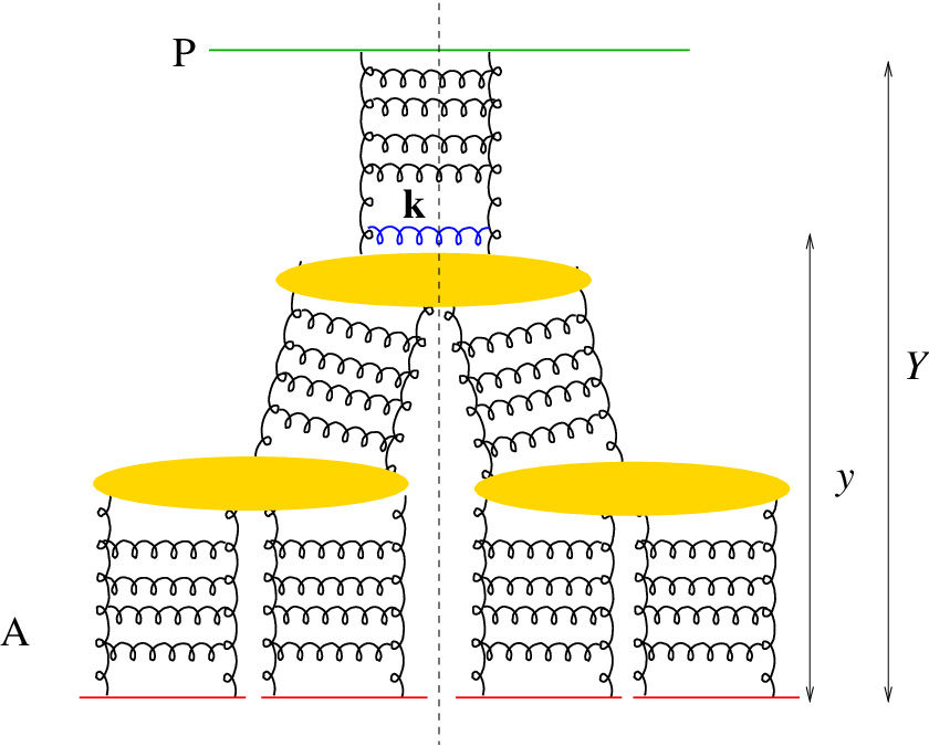
The relevant fan diagram is displayed in Fig. 2. We include the evolution effects using the method derived in [27]. We obtain the following generalization of (6):
| (7) |
where
| (8) |
Here has the meaning of the number of dipoles of size at rapidity and impact parameter generated by evolution from the original dipole having rapidity and impact parameter [63]. It satisfies the BFKL equation [66, 67]
| (9) |
with the initial condition
| (10) |
where we denoted and .
The forward elastic dipole–nucleus scattering amplitude satisfies the nonlinear BK equation [68, 69]
| (11) |
with the initial condition given by (5). In writing both equations (9) and (11) we assumed that the absolute value of impact parameter is much larger than the typical dipole size. This is a justified approximation for a scattering off a heavy nucleus.
In order to keep expressions as compact as possible, it is convenient to assume that the nuclear profile is cylindrical. This simple model allows correct identification of the atomic number (i.e. centrality) dependence of the cross sections. An explicit impact parameter dependence, which is required for numerical analysis, can be easily restored in the final expressions. Since we are not concerned here with the details of the impact parameter dependence, we integrate (9) over . The quantity
| (12) |
in turn satisfies the BFKL equation with the initial condition
| (13) |
In terms of , (7) reads
| (14) |
where is the cross sectional area of the interaction region.
The total cross section for diffractive gluon production is convenient to write in the following form
| (15) | |||||
where we introduced a new variable such that is the size of one of the daughter dipoles formed by emission of a gluon at point by a parent dipole .
III.2 Diffractive production with
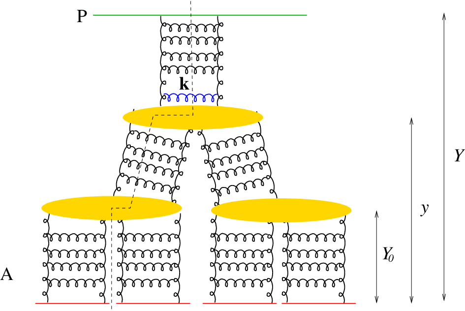
So far we have been concentrating on a case in which the rapidity of the produced gluon coincides with the rapidity gap in a diffractive event. In this case the diffractive scattering amplitude coincides with the square of the forward elastic scattering amplitude . In principle, a question may arise about the diffractive production of a gluon with . Such process is shown in Fig. 3. For the processes in which the transverse coordinate of the gluon in the amplitude is approximately the same as its coordinate in the c.c amplitude , the corresponding cross section is still given by (14)
| (16) |
where now in place of (8) we write
| (17) |
The amplitude equals to the cross section of single diffractive dissociation of a dipole of transverse size , rapidity and impact parameter on a target nucleus. It satisfies the Kovchegov–Levin evolution equation [70]
| (18) | |||||
with the initial condition
| (19) |
Diffractive gluon production of the kind shown in Fig. 3 requires a dedicated study and will certainly lead to a number of interesting observations. We are going to perform such analysis in future publications. In this paper we concentrate on the case .
IV Dipole evolution in onium and nucleus
IV.1 Dipole evolution in onium
Dipole evolution in onium is encoded in the function and is determined by solving equation (9) with the initial condition (10). In the case of a cylindrical profile we use function instead. The general solution of the BFKL equation for reads
| (20) |
where and the leading BFKL eigenvalue
| (21) |
with being the digamma function
| (22) |
The Mellin image can be found using the formula
| (23) |
The result is
| (24) |
Integral over can be done analytically in two important limits. In the leading logarithmic approximation (LLA) we expand the function near the minimum at as
| (25) |
where is the Riemann zeta function. Substituting (25) into (24) and integrating around the saddle point
| (26) |
we derive
| (27) |
where .
Alternatively, we can expand near one of its two symmetric poles at . This corresponds to the double logarithmic approximation. The choice of a particular pole depends on the relation between and . Expanding near we attain
| (28) |
Plugging this into (24) we have
| (29) |
The saddle point of the expression in the exponent is
| (30) |
which is valid only if . Expanding the argument of the exponential near the saddle point to the second order and integrating gives the double-logarithmic approximation
| (31) |
IV.2 Dipole evolution in a heavy nucleus
IV.2.1 Leading twist approximation
Consider the forward elastic dipole–nucleus scattering amplitude satisfying the nonlinear evolution equation (11). If the dipole size is much smaller than the saturation scale , then the quantum evolution of the amplitude is governed by the BFKL equation. Therefore in this case, the general solution is
| (35) |
The Mellin image of the amplitude is calculated as follows
| (36) | |||||
In the last line of (36) we used the fact that logarithmically depends on , see (3),(4). Analogously to the derivation of (27) we obtain in the leading logarithmic approximation
| (37) |
where the saddle point is
| (38) |
In the double logarithmic approximation (28) the saddle point for the case is
| (39) |
Repeating the by now familiar procedure we write
| (40) |
Next, we consider the case .
IV.2.2 Deep saturation region
Solution to the BK equation (11) deeply in the saturation regime was found in [71, 72, 73]. With the logarithmic accuracy the dominant dipole splitting corresponds to the configuration in which the size of one of the daughter dipoles () is much smaller than the other (see Sec. VI). Denote again and . In the saturation region we have either or the symmetric configuration . Both give equal contribution to the integral over . Restricting ourself to the case and doubling the integral we write the BK equation as follows:
| (41) |
Now, for the reason that in the saturation region, the amplitude is close to unity we render (41) as
| (42) |
The saturation scale can be found by equating the argument of the exponent in (40) to a constant which yields [71, 74]
| (43) |
Introducing a new scaling variable we solve (42) and find the high energy limit of the forward scattering amplitude (in the fixed coupling approximation). It reads [71]
| (44) |
where we approximated in the large limit. is the integration constant. It determines the value of the amplitude at the critical line .
V Diffractive cross section in the quasi-classical approximation
Careful inspection of (1) reveals that the cross section vanishes when size of the onium is much larger than the characteristic scale . This is in a sharp contrast with the inclusive gluon production case [26] where the cross section stays finite at . To understand the reason for such different behavior, consider a sample diagrams contributing to each of the processes shown in Fig. 4.
 |
 | |
| (a) | (b) |
In diagram (a), corresponding to the inclusive case, the propagator of the system in the nucleus is proportional to while the gluon emission amplitude is proportional to . Both do not involve the coordinate at all and are finite at . On the contrary, in diagram (b), corresponding to the diffractive case, the propagator involves both and coordinates, see (2), no factorization of dependence similar to the inclusive case happens. All other diagrams contributing to these two processes can be analyzed in the same way. Let us look at the color structure of the system in the two cases. By Pomeranchuk theorem, the exchanged (Coulomb) gluons are in the color singlet state. Therefore, we notice that in diagram (a) the system is in the color octet state and its propagator through the nucleus equals the propagator of a gluon dipole, whereas in diagram (b) the system is always in the color singlet state corresponding to the quark dipole. This feature can be seen also in expressions for the propagator, one involving the gluon saturation scale (inclusive case), another involving the quark saturation scale (diffractive case).
Now we would like to determine how does the diffractive cross section behave in the quasi-classical approximation. Consider the following integral appearing in the r.h.s. of (II) and (15):
| (45) | |||||
Let us analyze its behavior in the quasi-classical case () for small and large onium sizes.
V.1 Dilute regime
In the case of small onium we divide the entire integral over into three terms as follows:
| (46) | |||||
where (46) holds in logarithmic approximation. We can estimate each term utilizing the fact that according to (5)
| (47) |
Moreover, in the last two terms in (47) can be neglected since in most of the integration regions . Indeed, in the second term in the r.h.s. of (46) it can be seen once we neglect and expand at small . In the third term in the r.h.s. of (46) we have while . Accordingly, expanding the integrands using (47) we find that the first term in the r.h.s. of (46) is of the order , whereas the second and the third ones are of the order . Therefore, the last two terms in (46) dominate in the regime . It is customary to denote
| (48) |
which has the meaning of the gluon dipole forward elastic scattering amplitude. In terms of this quantity the function reads
| (49) |
where the lower limit of integration () has been set to zero with logarithmic accuracy (note that the second integral in the r.h.s. of (46) is dominated by dipoles of size ).
It is useful to notice, that (49) holds also in the case the low- evolution is taken into account. In the quasi-classical approximation the integral (49) can be done if we treat as a -independent constant neglecting its logarithmic variation. In that case, substituting (5) we derive
| (50) |
The cross section is obtained using (II) and (45). We have
| (51) |
V.2 Dense regime
As in the previous case we divide the integral into three parts
| (52) | |||||
Utilizing (47) we simplify (52) in the logarithmic approximation as follows
| (53) | |||||
| (54) |
Going from (53) to (54) we kept only the second term in the brackets in (53) as it is logarithmically enhanced. Formula (54) is valid in the case of low- evolution as well. Substituting (5) into (54) yields
| (55) |
Finally, the cross section follows from (II), (45) and (55) as
| (56) |
The striking feature of this formula is strong exponential suppression of diffractive gluon production for large onium. We will see in the next section that this result completely changes when the quantum evolution in the onium becomes an important effect.
VI Diffractive cross section including low- evolution
VI.1 Dilute regime
As in the quasi-classical case, first we are going to find the kinematic region which gives the largest (logarithmic) contribution to the integral. We have
| (58) | |||||
As has been noted in the previous sections, equations (49) and (54) hold also in the evolution case, provided the -dependence is explicitly indicated in the arguments of and . Generalization of (50) reads
| (59) |
where is a constant which depends on a particular functional form of and can be found numerically from (11). Using (44) in (54) gives another limit of function :
| (60) |
Accordingly, using (31) or (34) depending on the relation between and , i. e. if or if , as well as (59) and (60) we estimate that the second integral in (58) is enhanced by with respect to the first one, whereas the third integral is vanishingly small. Thus,
| (61) | |||||
Changing to a new integration variable defined as the integral in (61) can be taken explicitly in terms of the imaginary error function. In the double-logarithmic approximation the result reads
| (62) |
Both the quasi-classical result (51) and its quantum counterpart (62) show that the cross section is proportional to as required by the color transparency.
VI.2 Dense regime
Analogously to (58) we get
| (63) | |||||
The logarithmically enhanced contribution arises from the second integral which – upon substitution of (60) and (34) – becomes
| (64) |
Note that in the relevant kinematic region we can approximate . The integral over then becomes trivial yielding the final result
| (65) |
We observe that the cross section given by (65) is an increasing function of the rapidity interval between the onium and the nucleus. Together with the quasi-classical expression (56) it implies that the total cross section for the diffractive gluon production in a scattering of a large onium off the heavy nucleus is non-vanishing only if the low- evolution in onuim is an important effect. This can be seen directly in Fig. 2: the gluon multiplicity arises from the cut Pomeron attached to the onium. This observation has important phenomenological consequences as we discuss in the next section.
VII Discussion and summary
In this paper we discussed the coherent diffractive gluon production in high energy onium-nucleus collisions. The gluon multiplicity in the case of onium of small size is given by (51) and (62) and can be summarized as follows
| (66) |
where is a gluon distribution function at momentum scale . Gluon multiplicity vanishes in the limit as is required by the color transparency.
In the other limit of large onium, the gluon production cross section vanishes in the quasi-classical approximation as implied by (56). At the evolution effects in onium play increasingly important role. It is the cut Pomeron, connecting the onium and the dipole () emitting the triggered gluon, which contributes to the fast increase in gluon multiplicity as interval increases. One way to see it is to recall that during the linear evolution dipoles of various sizes are produced from the parent onium of size . We explained in (63) and (64) that the main contribution to the multiplicity stems from the dipoles of size no matter how big is the initial dipole . The resulting expression (65) has the following behavior
| (67) |
Dependence of the diffractive gluon multiplicity on the onium size is summarized in the Fig. 5.

To the extent that the large onium can serve as a model for proton, (56) and (65) describe the diffractive gluon production in proton-nucleus collisions. As such it has a direct implications to the RHIC and LHC phenomenology. Phenomenological studied show that the gluon saturation at RHIC starts to impact the gluon and valence quark spectra at rapidities (and larger). In our notations it corresponds to the rapidity interval between the gluon and the heavy nucleus and between the proton and the gluon. This corresponds to which is perhaps insufficient to have a sizable low- effect in proton implying a very low multiplicity of diffractive gluon production. On the other hand, exploring the backward rapidity region will not allow to probe the gluon saturation in the nucleus. Therefore, if the typical inter-quark distance in proton is larger than fm, then we do not expect a significant multiplicity of gluons in coherent diffraction of a proton on nucleus at RHIC, see Fig. 5. 11 1 Clearly, this conclusion does not hold if proton’s valence quarks form a diquark-quark configuration where the diquark has small size. From this perspective the diffractive gluon production at RHIC is a sensitive probe of the valence quark configuration in proton.
The situation radically changes at LHC where an additional rapidity window opens up. From the point of view of gluon saturation, the mid-rapidity in pA at LHC is expected to be similar to the rapidity at RHIC [32, 40]. At the same time, at the LHC midrapidity, which is certainly sufficient for the low- evolution to take place in proton. Therefore, we expect that measurements of the diffractive gluon production in pA collisions at LHC will be a sensitive probe of the low- dynamics. At EIC the typical dipole size is determined by the photon virtuality as which makes it possible the detailed study gluon saturation using the diffractive gluon production in different kinematical regions (see e.g. [75, 76]).
An interesting extension of our work is a case of diffractive production with small rapidity gap , which will be relevant at LHC. Of special interest is dependence of the differential cross section for diffractive gluon production on transverse momentum of produced gluon. We are addressing this and other issues in the forthcoming publication.
Acknowledgements.
K.T. is grateful to Yuri Kovchegov, Genya Levin and Jianwei Qiu for very informative and helpful discussions. The work of K.T. was supported in part by the U.S. Department of Energy under Grant No. DE-FG02-87ER40371. He would like to thank RIKEN, BNL, and the U.S. Department of Energy (Contract No. DE-AC02-98CH10886) for providing facilities essential for the completion of this work.References
- [1] L. D. McLerran and R. Venugopalan, Phys. Rev. D 49, 2233 (1994) [arXiv:hep-ph/9309289]; Phys. Rev. D 49, 3352 (1994) [arXiv:hep-ph/9311205]; Phys. Rev. D 50, 2225 (1994) [arXiv:hep-ph/9402335].
- [2] J. Jalilian-Marian, A. Kovner, A. Leonidov, and H. Weigert, Nucl. Phys. B 504, 415 (1997) [arXiv:hep-ph/9701284];
- [3] J. Jalilian-Marian, A. Kovner, A. Leonidov, and H. Weigert, Phys. Rev. D 59, 014014 (1999) [arXiv:hep-ph/9706377];
- [4] J. Jalilian-Marian, A. Kovner, A. Leonidov, and H. Weigert, Phys. Rev. D 59, 034007 (1999) [Erratum-ibid. D 59, 099903 (1999)] [arXiv:hep-ph/9807462];
- [5] J. Jalilian-Marian, A. Kovner, and H. Weigert, Phys. Rev. D 59, 014015 (1999) [arXiv:hep-ph/9709432];
- [6] A. Kovner, J. G. Milhano, and H. Weigert, Phys. Rev. D 62, 114005 (2000) [arXiv:hep-ph/0004014]; H. Weigert, Nucl. Phys. A 703, 823 (2002) [arXiv:hep-ph/0004044].
- [7] E. Iancu, A. Leonidov, and L. D. McLerran, Nucl. Phys. A 692, 583 (2001) [arXiv:hep-ph/0011241];
- [8] E. Iancu, A. Leonidov, and L. D. McLerran, Phys. Lett. B 510, 133 (2001) [arXiv:hep-ph/0102009];
- [9] E. Iancu and L. D. McLerran, Phys. Lett. B 510, 145 (2001) [arXiv:hep-ph/0103032];
- [10] E. Ferreiro, E. Iancu, A. Leonidov, and L. McLerran, Nucl. Phys. A 703, 489 (2002) [arXiv:hep-ph/0109115].
- [11] L. V. Gribov, E. M. Levin, and M. G. Ryskin, Phys. Rept. 100, 1 (1983).
- [12] A. H. Mueller and J. w. Qiu, Nucl. Phys. B 268, 427 (1986).
- [13] K. J. Golec-Biernat and M. Wusthoff, Phys. Rev. D 59, 014017 (1999) [arXiv:hep-ph/9807513].
- [14] K. J. Golec-Biernat and M. Wusthoff, Phys. Rev. D 60, 114023 (1999) [arXiv:hep-ph/9903358].
- [15] E. Gotsman, E. Levin, M. Lublinsky, U. Maor, and K. Tuchin, Phys. Lett. B492, 47 (2000) [arXiv:hep-ph/9911270].
- [16] E. Gotsman, E. Levin, M. Lublinsky, U. Maor, and K. Tuchin, arXiv:hep-ph/0007261.
- [17] E. Gotsman, E. Levin, M. Lublinsky, U. Maor, and K. Tuchin, Nucl. Phys. A697, 521 (2002).
- [18] Y. V. Kovchegov and L. D. McLerran, Phys. Rev. D 60, 054025 (1999) [Erratum-ibid. D 62, 019901 (2000)] [arXiv:hep-ph/9903246].
- [19] E. Levin and M. Lublinsky, Nucl. Phys. A 712, 95 (2002) [arXiv:hep-ph/0207374].
- [20] E. Levin and M. Lublinsky, Eur. Phys. J. C 22, 647 (2002) [arXiv:hep-ph/0108239].
- [21] J. Bartels, K. J. Golec-Biernat, and H. Kowalski, Phys. Rev. D 66, 014001 (2002) [arXiv:hep-ph/0203258].
- [22] D. Kharzeev and M. Nardi, Phys. Lett. B 507, 121 (2001) [arXiv:nucl-th/0012025];
- [23] D. Kharzeev and E. Levin, Phys. Lett. B 523, 79 (2001) [arXiv:nucl-th/0108006];
- [24] D. Kharzeev, E. Levin, and M. Nardi, arXiv:hep-ph/0111315.
- [25] D. Kharzeev, E. Levin, and M. Nardi, Nucl. Phys. A 730, 448 (2004) [Erratum-ibid. A 743, 329 (2004)] [arXiv:hep-ph/0212316].
- [26] Y. V. Kovchegov and A. H. Mueller, Nucl. Phys. B 529, 451 (1998).
- [27] Y. V. Kovchegov and K. Tuchin, Phys. Rev. D 65, 074026 (2002).
- [28] M. A. Braun, Phys. Lett. B 483, 105 (2000) [arXiv:hep-ph/0003003].
- [29] A. Dumitru and L. D. McLerran, Nucl. Phys. A 700, 492 (2002) [arXiv:hep-ph/0105268].
- [30] J. P. Blaizot, F. Gelis, and R. Venugopalan, Nucl. Phys. A 743, 13 (2004) [arXiv:hep-ph/0402256].
- [31] D. Kharzeev, E. Levin, and L. McLerran, Phys. Lett. B 561, 93 (2003) [arXiv:hep-ph/0210332].
- [32] D. Kharzeev, Y. V. Kovchegov, and K. Tuchin, Phys. Rev. D 68, 094013 (2003) [arXiv:hep-ph/0307037].
- [33] D. Kharzeev, Y. V. Kovchegov, and K. Tuchin, Phys. Lett. B 599, 23 (2004) [arXiv:hep-ph/0405045].
- [34] R. Baier, A. Kovner, and U. A. Wiedemann, Phys. Rev. D 68, 054009 (2003) [arXiv:hep-ph/0305265].
- [35] E. Iancu, K. Itakura, and D. N. Triantafyllopoulos, Nucl. Phys. A 742, 182 (2004) [arXiv:hep-ph/0403103].
- [36] F. Gelis and R. Venugopalan, Phys. Rev. D 69, 014019 (2004) [arXiv:hep-ph/0310090].
- [37] K. Tuchin, Phys. Lett. B 593, 66 (2004) [arXiv:hep-ph/0401022].
- [38] J. P. Blaizot, F. Gelis, and R. Venugopalan, Nucl. Phys. A 743, 57 (2004) [arXiv:hep-ph/0402257].
- [39] Y. V. Kovchegov and K. Tuchin, Phys. Rev. D 74, 054014 (2006) [arXiv:hep-ph/0603055].
- [40] K. Tuchin, Nucl. Phys. A 798, 61 (2008) [arXiv:0705.2193 [hep-ph]].
- [41] D. Kharzeev and K. Tuchin, Nucl. Phys. A 735, 248 (2004) [arXiv:hep-ph/0310358].
- [42] D. Kharzeev and K. Tuchin, Nucl. Phys. A 770, 40 (2006) [arXiv:hep-ph/0510358].
- [43] F. Gelis and A. Peshier, Nucl. Phys. A 697, 879 (2002) [arXiv:hep-ph/0107142].
- [44] A. Dumitru and J. Jalilian-Marian, Phys. Rev. Lett. 89, 022301 (2002) [arXiv:hep-ph/0204028].
- [45] J. Jalilian-Marian, Nucl. Phys. A 753, 307 (2005) [arXiv:hep-ph/0501222].
- [46] R. Baier, A. H. Mueller and D. Schiff, Nucl. Phys. A 741, 358 (2004) [arXiv:hep-ph/0403201].
- [47] J. Jalilian-Marian, Nucl. Phys. A 739, 319 (2004) [arXiv:nucl-th/0402014].
- [48] M. A. Betemps and M. B. Gay Ducati, Phys. Rev. D 70, 116005 (2004); Phys. Lett. B 636 (2006) 46.
- [49] Y. Li and K. Tuchin, Phys. Rev. D 75, 074022 (2007) [arXiv:hep-ph/0702208].
- [50] K. Tuchin, Nucl. Phys. A783, 173 (2007) [arXiv:hep-ph/0609258].
- [51] J. Jalilian-Marian and Y. V. Kovchegov, Prog. Part. Nucl. Phys. 56, 104 (2006) [arXiv:hep-ph/0505052].
- [52] M. Wusthoff, Phys. Rev. D 56, 4311 (1997) [arXiv:hep-ph/9702201].
- [53] J. Bartels, H. Jung, and M. Wusthoff, Eur. Phys. J. C 11, 111 (1999) [arXiv:hep-ph/9903265].
- [54] B. Z. Kopeliovich, A. Schafer, and A. V. Tarasov, Phys. Rev. D 62, 054022 (2000) [arXiv:hep-ph/9908245].
- [55] Y. V. Kovchegov, Phys. Rev. D 64, 114016 (2001) [Erratum-ibid. D 68, 039901 (2003)] [arXiv:hep-ph/0107256].
- [56] K. J. Golec-Biernat and C. Marquet, Phys. Rev. D 71, 114005 (2005) [arXiv:hep-ph/0504214].
- [57] C. Marquet, Nucl. Phys. B 705, 319 (2005) [arXiv:hep-ph/0409023].
- [58] C. Marquet, Phys. Rev. D 76, 094017 (2007) [arXiv:0706.2682 [hep-ph]].
- [59] S. Munier and A. Shoshi, Phys. Rev. D 69, 074022 (2004) [arXiv:hep-ph/0312022].
- [60] A. Kovner, M. Lublinsky, and H. Weigert, Phys. Rev. D 74, 114023 (2006) [arXiv:hep-ph/0608258].
- [61] A. Kovner and U. A. Wiedemann, Phys. Rev. D 64, 114002 (2001) [arXiv:hep-ph/0106240].
- [62] B. Z. Kopeliovich, A. V. Tarasov, and A. Schafer, Phys. Rev. C 59, 1609 (1999) [arXiv:hep-ph/9808378].
- [63] A.H. Mueller, Nucl. Phys. B415, 373 (1994); A.H. Mueller and B. Patel, Nucl. Phys. B425, 471 (1994); A.H. Mueller, Nucl. Phys. B437, 107 (1995).
- [64] A.H. Mueller, Nucl. Phys. B335, 115 (1990).
- [65] V. A. Abramovsky, V. N. Gribov, and O. V. Kancheli, Yad. Fiz. 18, 595 (1973) [Sov. J. Nucl. Phys. 18, 308 (1974)].
- [66] E. A. Kuraev, L. N. Lipatov, and V. S. Fadin, Sov. Phys. JETP 45, 199 (1977) [Zh. Eksp. Teor. Fiz. 72, 377 (1977)].
- [67] I. I. Balitsky and L. N. Lipatov, Sov. J. Nucl. Phys. 28 (1978) 822 [Yad. Fiz. 28 (1978) 1597].
- [68] I. Balitsky, Nucl. Phys. B 463, 99 (1996) [arXiv:hep-ph/9509348].
- [69] Y. V. Kovchegov, Phys. Rev. D 60, 034008 (1999) [arXiv:hep-ph/9901281].
- [70] Y. V. Kovchegov and E. Levin, Nucl. Phys. B 577, 221 (2000) [arXiv:hep-ph/9911523].
- [71] E. Levin and K. Tuchin, Nucl. Phys. B 573, 833 (2000) [arXiv:hep-ph/9908317].
- [72] E. Levin and K. Tuchin, Nucl. Phys. A 691, 779 (2001) [arXiv:hep-ph/0012167].
- [73] E. Levin and K. Tuchin, Nucl. Phys. A 693, 787 (2001) [arXiv:hep-ph/0101275].
- [74] J. Bartels and E. Levin, Nucl. Phys. B 387, 617 (1992).
- [75] E. Gotsman, E. Levin, U. Maor, L. D. McLerran, and K. Tuchin, Phys. Lett. B 506, 289 (2001) [arXiv:hep-ph/0008280].
- [76] E. Gotsman, E. Levin, U. Maor, L. D. McLerran, and K. Tuchin, Nucl. Phys. A 683, 383 (2001) [arXiv:hep-ph/0007258].