Improved search for - mixing using semileptonic decays at Belle
Abstract
A search for mixing in the neutral meson system has been performed using semileptonic and decays. Neutral mesons from decays are used and the flavor at production is tagged by the charge of the slow pion. The measurement is performed using 492 fb-1 of data recorded by the Belle detector. From the yield of right-sign and wrong-sign decays arising from non-mixed and mixed events, respectively, we measure the ratio of the time-integrated mixing rate to the unmixed rate to be . This corresponds to an upper limit of at the C.L.
pacs
14.40.Lb, 13.20.Fc, 12.15.FfI INTRODUCTION
The phenomenon of mixing has been well established in the -, - and - systems. Recently, evidence for mixing in the - system has been obtained with a statistical significance of more than three standard deviations for the first time [1, 2]. In addition, several new measurements help constrain the relevant mixing parameters [3, 4]. The parameters used to characterize - mixing are and , where and are the differences in mass and decay width between the two neutral charmed meson mass eigenstates, and is the mean decay width. The mixing rate within the Standard Model is expected to be small [5]: the largest predicted values, which include the impact of long distance dynamics, are of the order .
For and negligible violation, the time-dependent mixing probability for semileptonic decays has the following form [6]:
| (1) |
where is the ratio of the time-integrated mixing probability to the time-integrated non-mixing probability:
| (2) |
The mixing rate can be measured directly by using semileptonic decays of mesons. The most stringent constraint from semileptonic decays, at the 90% confidence level, comes from our previous measurement [7]. Other measurements of using semileptonic decays are less sensitive [8, 9, 10], whereas results from hadronic decays are more precise [11, 12, 13]. In this paper we present an improved search for - mixing using semileptonic decays of charmed mesons, which supersedes our previous measurement [7]. We measure in a 492 data sample recorded by the Belle detector at the KEKB asymmetric-energy collider [14], at a center-of-mass (cms) energy of 10.58 GeV. The Belle detector [15] is a large-solid-angle magnetic spectrometer that consists of a silicon vertex detector (SVD), a 50-layer central drift chamber (CDC), an array of aerogel threshold Cherenkov counters (ACC), a barrel-like arrangement of time-of-flight scintillation counters (TOF), and an electromagnetic calorimeter (ECL) comprised of CsI(Tl) crystals located inside a superconducting solenoid coil that provides a T magnetic field. An iron flux-return located outside of the coil is instrumented to detect mesons and to identify muons (KLM). Two different inner detector configurations were used. The first 140 of data were taken using a 2.0 cm radius beam-pipe and a 3-layer silicon vertex detector (SVD-1), and the subsequent 352 were taken using a cm radius beam-pipe, a 4-layer silicon detector (SVD-2) and a small-cell inner drift chamber [16].
To study signal and background distributions we use Monte Carlo (MC) simulated samples [17] in which the number of selected events is about 2.7 times larger than in the data sample.
II RECONSTRUCTION OF DECAYS
We select mesons arising from decays and reconstruct them as , where can be either an electron or muon [18]. The notation denotes a pion, i.e., the pion that originates from the . The average momentum of this pion is only about 0.23 GeV, whereas the average momentum of the lepton and kaon from the signal decay are 0.96 GeV and 1.52 GeV, respectively. The momenta given in this paper are measured in the laboratory frame, unless otherwise stated; momenta measured in the cms frame are denoted with an asterisk, e.g., . The reconstruction of mesons in this specific decay chain enables tagging of the meson flavor at production using the charge of the slow pion .
There are three detected particles in the final state: , and , where can be either a muon or an electron. The non-mixed decay results in a charge combination , which we refer to as the Right-Sign (RS) charge combination. The mixing process results in , which we refer to as the Wrong-Sign (WS) charge combination, as summarized in Table 1.
| charge combination | process | name |
|---|---|---|
| non-mixed | Right-Sign, RS | |
| mixed | Wrong-Sign, WS |
Because the neutrino is not directly reconstructed, the masses of the and candidates are smeared. However, by calculating the difference between the two masses, the uncertainty due to the neutrino four momentum cancels to a large extent. Thus
| (3) |
the reconstructed invariant mass difference between the and the meson, is the most appropriate observable to extract the number of signal events. For signal events, the distribution of peaks at 0.145 GeV, the mass difference between the and meson (see Fig. 1).
II.1 Selection criteria
Among all the different processes occurring in collisions, hadronic final states are selected with an efficiency above 99%. The selection is based on the energy of the charged tracks and neutral clusters, total visible energy in the cms system, the component (opposite to the positron beam direction) of the total cms momentum, and the position of the reconstructed event vertex [19].
Using MC simulation, the criteria to select the signal decays are optimized to give the best significance for the extracted number of mixed (WS) events, . The uncertainty is due to the fluctuation of the background in the region GeV/; the fluctuation of the signal events at the rate of our previously measured upper limit [7] is negligible. Hence we maximize
| (4) |
Since the kinematic properties of mixed and non-mixed events are the same, in the optimization the RS signal is used instead of the WS signal. The optimal values for the selection criteria in some observables are correlated and hence the final criteria are obtained by iterative optimization. In the optimization, selection criteria based on the proper decay time are also included, as described in Sec. III.
We suppress mesons arising from events in order to avoid the situation in which the selected sample would be composed of two subsamples with different kinematic properties. These events have different kinematic properties from the decays of mesons produced in (continuum events), and a different apparent decay length between the interaction point and the decay vertex, because of the finite lifetime. As a result, the mesons from this source have slightly different resolutions in kinematic variables, and their proper decay time cannot be measured in the same way as for mesons from the continuum. Since the fraction of mesons from decays is smaller than that from the continuum production, and the background contribution from decays is large, the sensitivity to mixed events is not reduced by rejecting candidates from decays.
The quantity used to discriminate between events (spherical) and continuum events (jet-like) is the ratio of the second to zeroth Fox-Wolfram moment, [20]. To suppress candidates from decays we demand . A further effective rejection of events is described below.
Tracks with an impact parameter with respect to the interaction point in the radial direction, cm, and in the beam direction, cm, are considered as candidates. These criteria remove badly reconstructed tracks and tracks not arising from the interaction point. A slow pion candidate is required to have a momentum smaller than 600 MeV/. To reduce the background from electrons, we require the electron identification likelihood (based on the information from the CDC, ACC and ECL [21]) of a candidate to be , which selects slow pions with an efficiency of 96% and rejects 72% of electrons. The total efficiency of the slow pion selection criteria and tracking is 51%.
Electron candidates are required to have momenta greater than 250 MeV/ and an electron identification likelihood . The efficiency of the identification criterion is 76%; in total around 46% of all generated signal electrons are retained. Muon candidates are required to have momentum greater than 650 MeV/ and the muon identification likelihood (based on information from the KLM and properties of the track [22]) ; the latter criterion selects muons in the chosen momentum range with an efficiency of 67%. These two requirements are highly correlated since the identification efficiency of muons with momenta lower than 600 MeV/ is very poor. The efficiency of the above selection criteria and tracking is 30%.
Kaon candidates are required not to satisfy the lepton selection criteria. Kaons from decays should have and kaons from decays . The difference in this requirement is due to the correlation between lepton momenta and kaon momenta that enters through other kinematic variables, and due to different background contributions in both decay modes. A combined likelihood for a given track to be a , or is obtained based on the information from the TOF, CDC and ACC [19]. Kaon candidates are selected using (efficiency of 87% for signal kaons in the selected momentum range) and (efficiency of 99% for signal kaons). Around 42% of all generated kaons in the electron decay mode, and around 48% in the muon decay mode pass the selection criteria.
At this stage, about 17.0% of all generated decays, and about 12.5% of all generated decays, are reconstructed. Further criteria are applied to improve the sensitivity to mixed events. In the following, these criteria are described and for each of them the signal loss and the background rejection factors are given.
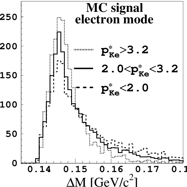
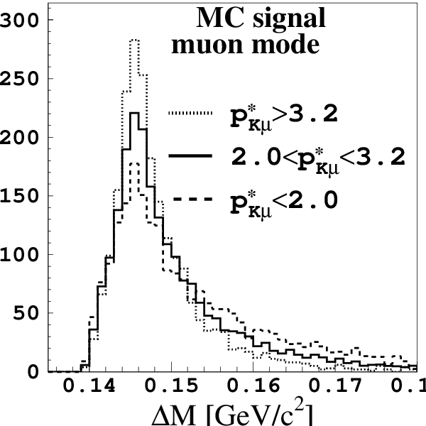


The most effective requirement is the one on the sum of the kaon and lepton momenta, calculated in the cms system, , see Fig. 2. Its optimized value is between 1.7 and 1.9 GeV. However, simulated signal events show a clear improvement in the resolution at higher values, see Fig. 1. The full width at half maximum (FWHM) of the simulated distribution reduces from 8.6 MeV/ for GeV/ to 6.9 MeV/ for GeV/ in the electron decay mode, and from 7.7 MeV/ to 5.2 MeV/ for the same intervals in the muon decay mode. Hence is required to be at least GeV/, a value that also eliminates a large fraction of meson decays arising from events. This requirement results in a signal loss of 28% in the electron decay mode and 23% in the muon decay mode, while rejecting 76% of the total background in the electron decay mode and 67% of the total background in the muon decay mode.
We apply a selection on the invariant mass of the kaon-lepton system. For the electron decay mode the optimal range is and for the muon decay mode , see Fig 3. In the electron decay mode this requirement rejects 25% of the total background at a cost of losing 5.5% of signal events. In the muon decay mode the signal loss is higher, 12%, but so is the background rejection, 44%.


decays to two mesons in the final state are an important source of background. There are four such decays (see Table 2). Their branching fractions are at least one order-of-magnitude larger than the effective branching fraction for . Although particle identification reduces their presence in the final sample, it is still important to suppress this background, because its distribution has a shape similar to that of the signal. Background exhibiting a peak around 0.145 GeV is called peaking background and reduces the sensitivity to mixed events much more than the non-peaking background.
| decay mode | Br [] [23] | contribution to WS |
|---|---|---|
| , | ||
| , |
In the electron decay mode, the requirement on rejects 90% of the background arising from the doubly Cabibbo suppressed decay , through misidentification of the pion as an electron; in the muon decay mode the suppression rate for this background is 98%. In both decay modes it completely eliminates the background due to misidentification of both pions from .
The Cabibbo-favoured decays contribute to the WS background if the kaon is misidentified as a lepton and the pion is misidentified as a kaon. To suppress this type of background, the invariant mass of the kaon-lepton system, , is calculated with the pion mass assigned to the kaon candidate and the kaon mass assigned to the lepton candidate. If in the electron decay mode, and in the muon decay mode, the candidate is rejected. Here is the mass of the meson, 1.8645 GeV/ [23]. In the electron decay mode, this requirement rejects of the WS background from decays, and in the muon decay mode.
To suppress the contribution from decays ( being misidentified as a lepton), the invariant mass of the kaon-lepton system, , is calculated with the kaon mass assigned to both candidates. If in the electron decay mode, and in the muon decay mode, the candidate is rejected. In the electron decay mode, this requirement rejects of the WS background from decays, and in the muon decay mode .
The requirements on and result in a signal loss of 3% in the electron decay mode and 2% in the muon decay mode. The rejection of the total background in both decay modes is similar to the signal loss.
II.2 Rejection of
An important source of background is due to electrons from photon conversions: either the electron candidate, the slow pion candidate, or both, may be due to tracks.


In the electron WS sample, both the slow pion and the signal electron candidates can come from , and such events tend to have low values (Fig. 4, left). To suppress this background we calculate , the invariant mass of the system with the electron mass assigned to both tracks. We reject candidates with GeV. The requirement rejects more than 99% of this background, see Fig. 4, right. To retain equal reconstruction efficiencies for the mixed and non-mixed events, this requirement is implemented in both RS and WS samples.
Background from , where one electron from the first photon and one electron from the other photon are taken as the electron and slow pion candidate, exhibits similar behavior to the case where the electrons are both from the same photon. This background is also successfully eliminated by the above selection.
Assuming that the signal electron candidate comes from , in the electron decay mode we perform a search for the other electron among all the other tracks in the event with the opposite charge to the signal electron candidate. If , the mass of the system, is below 80 MeV, the electron candidate is rejected.
Assuming that the slow pion candidate is a misidentified electron from , we perform a search for the other electron () among all the other tracks in the event. The other electron should have the opposite charge to the slow pion candidate, and an electron likelihood to reduce rejection of true signal slow pions. If , the mass of the system with the electron mass assigned to both tracks, is below 80 MeV, the slow pion candidate is rejected. This photon conversion rejection is performed for slow pion candidates in both the electron and muon decay modes and results in around 0.4% signal loss and rejects around 2.4% of the total background.
In total, the rejection of photon conversion in the electron decay mode results in a 14% signal loss and 32% rejection of the total WS background.
II.3 Neutrino reconstruction
Four-momentum conservation in collision implies
| (5) |
for the signal decay, where stands for the cms four-momentum of the system and indicates the four-momentum of all detected particles except the charged kaon and the lepton candidates [24]. Eq. (5) is true if all the particles produced in the collision are detected. As the Belle detector covers nearly the entire solid angle around the interaction point, neutrino reconstruction can be successfully performed.
The variable is calculated using all the remaining charged tracks (except the kaon and lepton candidates) with cm and cm, and photons with an energy above MeV. Mass is assigned to a track according to the following criteria:
- •
A track is assigned the electron mass if its electron likelihood is .
- •
A track is assigned the muon mass if and its muon likelihood is .
- •
A track is assigned the kaon mass if , and .
- •
A track is assigned the proton mass if , , and .
- •
In all other cases the track is assigned the charged pion mass [25].
A first approximation for the neutrino four-momentum is obtained using Eq. (5) and the resulting distribution for signal events is shown in Fig. 5 (left) with the dashed line. It peaks at around GeV/, a value close to the mass difference, GeV/, and has a FWHM of 58 MeV/.
Two kinematic constraints are used to improve the resolution on the neutrino momentum. To simplify the expressions, we performed the calculation in the cms system, since . First, the squared invariant mass of the selected particles is calculated using . The distribution of is shown in Fig. 6, left. For signal events, the invariant mass should equal . To reject poorly reconstructed events, exhibiting a large FWHM of the final distribution, only candidates with GeV GeV are retained. For the selected events, is rescaled by a factor requiring
| (6) |
The neutrino four-momentum is then recalculated as , and a corrected is obtained, where has been forced to equal . With this correction, the distribution has a FWHM of 11 MeV/ in the electron decay mode and 10 MeV/ in the muon decay mode; the improvement is shown in Fig. 5 (left). The distribution of the scale factor for events in the finally selected sample is shown in the left plot of Fig. 7. It peaks at around 1.04 for the electron decay mode and 1.06 for the muon decay mode. The average in both decay modes is around 1.3.


As a second kinematic constraint, the square of the missing mass, , is used. The distribution of is shown in Fig. 6, right. For events satisfying GeV GeV, the angle between the direction of and the direction of is corrected in order to yield
| (7) |
expressed in terms of energies and magnitudes of three-momenta this yields
| (8) |
The angle is corrected by rotating in the plane determined by the vectors and . The distribution of the correction angle for the finally selected signal events is shown in the right plot of Fig. 7. It has a peak at around and an average value of . The final neutrino four-momentum is calculated with the rescaled and rotated , using Eq. (5).
The requirements on and result in a signal loss of 4.5% in the electron decay mode and 4.1% in the muon decay mode while rejecting 9.7% in of background in the electron decay mode and 8.9% of the background in the muon decay mode.


The distribution obtained using the neutrino four-momentum after the use of kinematic constraints is shown in Fig. 5 (left) as the solid line. The resolution is significantly improved, with the FWHM being about 6.6 MeV/ for the electron decay mode and 6.2 MeV/ for the muon decay mode. Using the MC-simulated background events, it has been verified that such a neutrino reconstruction does not induce any peaking in the background distribution. From the right plot in Fig. 5 it can be seen that the number of background events in the signal region () after applying the constraints only slightly exceeds the number of events without the constraints (by 8.1% in the electron decay mode and 16.6% in the muon decay mode).


For candidates we require , which retains 97.4% signal events in the electron decay mode and 97.8% in the muon decay mode.
II.4 combined with both and
After all the above requirements are applied, a small fraction of events contain a candidate that has been combined with slow pions of opposite charges to form both RS and WS candidates. Events in which such candidates are found are rejected. This veto results in a signal loss of about 2.6% in both electron and muon decay mode. For the former it rejects 18% of background events and for the latter about 13%.
At this stage the efficiency for
reconstructing the signal with GeV/ is found
to be for the electron decay mode and for
the muon decay mode. The quoted errors include a small variation of
efficiency depending on the detector conditions.
A summary of the applied selection criteria is presented in Table 3. Since the non-mixed and mixed processes have the same kinematics, the WS and RS efficiencies for all the described selection criteria are the same.
| electron decay mode | muon decay mode | |
| event | ||
| impact parameter: cm, cm | ||
| electron likelihood 0.1 | ||
| electron likelihood 0.95 | muon likelihood 0.97 | |
| / | ||
| recon. | GeV GeV | |
| GeV GeV | ||
| reject combined with both and | ||
III PROPER DECAY TIME
As the proper decay time distribution of WS background events tends to have lower values than that of WS signal events, the proper decay time of a meson can be used to select possible mixed events with a higher purity. Since the information on the proper decay time is used only to increase the sensitivity to WS events, modeling of the proper decay time distribution is not detailed. We do not account for the fact that the associated signal decays (defined in Sec. IV) have a slightly different proper decay time resolution function than the signal decays, or for the fact that the resolution depends slightly on the true value of the proper decay time. The effects of these two assumptions were studied carefully; the differences between data and the modeling functions are taken into account in the systematic uncertainties and lead to a negligible change of the final result.
The dimensionless proper decay time (proper decay time in units of ps [23]) is calculated from the flight distance and its momentum :
| (9) |
The momentum is calculated by summing the momenta of the daughter particles. The flight distance is the distance between the production vertex, , and its decay vertex, . The decay vertex is obtained by fitting the kaon and lepton tracks to a common vertex. The production vertex is obtained by extrapolating the momentum vector to the interaction region. The position and width of this region are determined over a large number of interactions for which the KEKB beam conditions do not change significantly.
According to MC simulation, the resolution on the proper decay time is improved if the flight distance is calculated as the projection of the vector on the normalized momentum vector. Since the interaction region is much narrower in the radial direction, we use only the radial components ( and ) to measure the proper decay time. The radial flight distance is calculated as
| (10) |
The proper decay time is then evaluated as
| (11) |
The observed distribution is smeared due to the experimental resolution. As the data recorded with the SVD-2 configuration has a slightly narrower resolution function than the data taken with the SVD-1 configuration, we perform the measurements of separately for both subsamples. Thus we have four subsamples: the electron subsamples are denoted by e-1 and e-2 for the SVD-1 and SVD-2 configurations, respectively. Similarly the muon subsamples will be denoted as -1 and -2.
III.1 Distribution of signal events
We obtain the resolution function for signal events from the data, using the RS decays. To be able to do so, we first determine the shape of the distribution for RS background events, which is shown in Fig. 8, right, as the dashed line. This distribution is also obtained from the data, as described in the following.
The normalized function that describes the distribution of RS background events is
| (12) |
It is composed as a sum of an exponential function with the decay time and a delta function (their fractions are determined by the parameter ), convolved with a detector resolution. The latter is phenomenologically described by a sum of the Lorentz function and an asymmetric Lorentz function (both are explicitly given in the Appendix, Eq. (28) and (VI)); , and are their width parameters and determines their fractions in the resolution function. A wide Lorentz function is added to describe the decay times measured from badly reconstructed tracks (outliers); its width parameter is and its fraction in the total sample . The convolutions are performed numerically by substituting the integral with a sum. It has been verified that the numerical accuracy is satisfactory, i.e. not affecting the result.
To determine the eight free parameters of the function from the data, we divide the range into 15 intervals as shown in Fig. 8, left. In each of these 15 intervals we extract the number of RS background events, , by performing fits to the distribution of RS events. The fit to the distribution is described in detail in Sec. IV.2. The errors include the systematic error due to the finite number of MC simulated events and the uncertainty of the correlated background fraction in the total RS background.
If we divide in one of the 15 intervals by the total number of background events (the sum over the 15 intervals), the obtained fraction is expected to agree with the integral of (Eq. 12) over that interval.
Hence we calculate in all 15 intervals and determine the eight free parameters of by a fit to these fractions. The value of the fitting function in each interval is calculated as the integral of over that interval. The fractions and the result of the fit for the e-2 subsample are shown in Fig. 8, left plot; the obtained background distribution is shown with the dashed line in the right plot. The reduced values of the fits are reasonable, ranging from 0.4 to 4 for 7 degrees of freedom. The uncertainties on the fitted parameters of the RS background proper decay time distribution are taken into account when calculating the uncertainty of the result, .
III.1.1 RS signal distribution
The proper decay time distribution for RS events is described by
| (13) |
where is the total number of RS events and is the signal fraction, obtained from a fit to in the entire proper decay time region. The values are , , and for e-1, e-2, -1 and -2 subsamples, respectively. The function describes the shape of the RS signal events, which is an exponential convolved with the resolution function,
| (14) |
The resolution function is parameterized as
| (15) |


Here is the Gaussian function. The six free parameters of the resolution function for the RS signal events are , , , , and . They are obtained by a fit of to the proper decay time distribution of RS events. In this fit, the parameters of are fixed to the values previously obtained and , the dimensionless decay time, is fixed to 1.0. An example of a fit result is shown in the right plot of Fig. 8. The reduced values range between 1.2 and 2.4 for 194 degrees of freedom and exhibit a slight disagreement between the fitting model and the data. The disagreement is accounted for in the systematic error evaluation, resulting in a negligible change of the final result.
III.1.2 WS signal distribution
Since decays of the mixed and of the unmixed mesons have the same kinematic properties, the proper decay time resolution function for both is assumed to be the same. Hence from the RS signal resolution function, , the proper decay time distribution for WS signal events is calculated:
| (16) |
where is the corresponding normalization constant and is fixed to 1.


To select the interval with the highest sensitivity to mixed events, the ratio given in Eq. (4) is maximized. In this optimization we use the calculated distribution for WS signal events, (Eq. (16)); for the background we use the distribution of the WS events from the data. Even if the latter contains some mixed events, the effect on the result of the optimization is negligible, since mixing is small. The distributions of background events, WS signal events and the figure-of-merit can be seen in Fig. (9). The optimal proper decay time intervals for the four subsamples range between 1.6–1.7 and 8.9–9.5. In order to keep the measurement method uniform, we select a common interval for all four subsamples,
| (17) |
In this interval, about 70% of WS signal events are selected, while rejecting about 80% of background events (the values are similar in each of the four subsamples).
III.2 Extraction of and further improvement
Because the proper decay time distribution of the RS signal events () is different from that of the WS signal events (), after the application of a selection based on proper decay time, the ratio is obtained as
| (18) |
where are the numbers of extracted signal events without the selection, and are the numbers of extracted signal events in the selected interval. The superscript labels different intervals. The efficiencies are obtained by integrating the proper decay time distribution of the RS signal events, , over the selected interval. Similarly, the efficiencies are obtained from the calculated proper decay time distribution of the WS signal events, . The ratios are listed in Table 7. The errors on the efficiencies quoted there include the uncertainty on the fraction of the RS correlated background (as defined in Sec. IV.1), the statistical and systematic uncertainty on the signal fraction in the RS sample, the statistical and systematic uncertainties in the parameters of the RS background and signal distributions and the uncertainties in the world averages of and [23]. The resulting errors on the measured parameter are included in the systematic uncertainty and are negligible. Imperfections in modelling the decay time distributions are included as a separate source of a systematic uncertainty as described below.
To further exploit the proper decay time information, we divide the chosen range (Eq. (17)) into six intervals, with boundaries at 1.6, 2.0, 2.5, 3.1, 4.0, 5.6, and 9.0. The binning is chosen so as to have approximately the same number of events in each interval. The mixing rate is measured in each of the six intervals and the measurements are expected to be consistent. Due to the additional proper decay time information the sensitivity of the final result is expected to be improved in comparison with the sensitivity of a single measurement in the total range.
IV SIGNAL YIELD EXTRACTION
According to the MC simulation, the selected sample of RS events includes many candidates from semileptonic decays other than , combined with the correctly reconstructed slow pion. The most important of these decays are:
- •
,
- •
, followed by ,
- •
,
- •
, followed by ,
- •
, followed by .
The final state lepton in these decays is of the same charge as in the decay , so its charge can be used to tag mixing in the same way. In the last three decays with a instead of the in the final state, the pion is misidentified as a kaon. The selected sample also includes candidates where the semileptonic decay is correctly reconstructed, but the slow pion decays in flight to a muon, , and then the muon is misidentified as the slow pion. The muon has the same charge as the slow pion and can be used to tag the flavor at production in the same way as the slow pion. Hence all these processes are treated as part of the signal and will be referred to as associated signal decays.
According to MC simulation, the associated signal decays have a similar distribution to the decays. Due to unreconstructed or misidentified particles in these final states, the FWHM of the distribution is larger, 12.3 MeV in the electron decay mode and 14.3 MeV in the muon decay mode (see Fig. 10). For the same reasons, the proper decay time distribution is slightly different from that for the signal. The fraction of the associated signal decays in the sample of all reconstructed signal decays can be found in Table 4. There is also a small fraction of signal events (around 1%) from events. Due to the lower average momentum of mesons from decays, the distribution for signal events from decays is slightly wider than that for signal events from events; it is similar to the distribution of the associated signal decays.


| assoc. sig. [%] | sig. from decays [%] | |||||||
|---|---|---|---|---|---|---|---|---|
| all | all | |||||||
| 16.58 | 0.05 | 17.7 | 0.1 | 1.20 | 0.01 | 1.18 | 0.03 | |
| 11.54 | 0.04 | 12.3 | 0.1 | 1.07 | 0.01 | 1.04 | 0.03 | |
IV.1 Background
The background is divided into two categories: the correlated background and the uncorrelated background. The shapes of both background components can be seen in Fig. 11.
Correlated background is the background where the lepton candidate or the kaon candidate, or both, originate from the same decay chain as the slow pion candidate. The angular correlation between the slow pion and candidates leads to a concentration of events at low values of .
The remaining, uncorrelated background has a distribution that rises steadily from threshold, as the available phase space increases. This component is dominant, especially in the WS sample (see Table 5). The fraction in the muon decay mode is larger than in the electron decay mode, because the probability for a kaon or a pion to be misidentified as a muon is larger than the probability to be misidentified as an electron. The fraction is larger in the RS sample than in the WS sample due to the larger branching fractions of the Cabibbo favored decays. Selecting the proper decay time interval , decreases the fraction of the correlated background in the total background. According to MC simulation, the correlated background has three components: background from decays, which has the largest fraction and is the most strongly peaked of the three, background from , decays in which one of the two electrons from conversion is taken as a slow pion candidate, and background from decays, where one of the pions is taken as the slow pion candidate and the other is assigned as a kaon or lepton candidate.
| Right Sign sample | Wrong Sign sample | |||||||
|---|---|---|---|---|---|---|---|---|
| all | all | |||||||
| 34.49 | 0.07 | 25.33 | 0.15 | 7.22 | 0.05 | 5.64 | 0.10 | |
| 40.07 | 0.06 | 39.62 | 0.14 | 14.87 | 0.06 | 14.76 | 0.14 | |


The distribution for the total RS background can be seen in Fig. 12 as the dashed line. To fit the distribution of the data as explained in Sec. IV.2, the distribution of the RS background events is obtained from MC simulation.
The distribution for the total WS background is shown in Fig. 11 as the solid histogram. One can see that the difference in shape between the uncorrelated background and the total background is smaller in the electron decay mode than in the muon decay mode. This is both due to the larger correlated background component in the muon decay mode (see Table 5) and due to its shape, shown in the same figure.
To check the MC simulation and to avoid systematic errors arising from any discrepancy with the data, the uncorrelated background in the WS sample was described using the data. This background is modeled by combining slow pion candidates and candidates from different events. Technically this is done by embedding slow pion candidates into other events according to the following procedure:
- •
All slow pion candidates from an event in which a candidate was found, are taken to be embedded into other events.
- •
We denote by the number of slow pion candidates which form a WS combination in their original event, and their charge by . Slow pions are embedded only into events with the same value of and only the embedded slow pions of charge are used to form the WS combinations.
- •
For each value of , slow pion candidates from different events are stored to be embedded into other events.
- •
Each candidate is combined with slow pions from several other events; slow pions from a maximum of events are used. Once a combination satisfying all the requirements is obtained (including ), further combinations are not formed.
- •
Once an embedded slow pion is used to form a combination satisfying all the requirements, none of the remaining slow pions from the same event is embedded into other events.
With these requirements, the distribution of the sample of embedded slow pions slightly depends on , the maximum number of events from which the embedded slow pions are taken and tested with a single candidate. The dependence is due to the dependence on the slow pion momentum. Slow pions with higher momenta tend to form candidates with slightly higher values, hence their probability to form a candidate with is smaller. Increasing enables these slow pions to be tested with a larger number of candidates and enhances the probability to form a combination with . Thus increasing slightly enhances the contribution at higher values.
The most appropriate value is determined from the data by observing samples of . In this proper decay time region, the expected fraction of the mixed signal events in the WS background is much smaller (around 18 times in the electron and around 27 times in the muon decay mode) than in the region . Hence it is safe to assume that the WS data sample of contains no mixed signal events. For we combine the SVD-1 and SVD-2 subsamples and compare the distribution of the WS data with the distribution of the subsample used to describe the WS background, embedded slow pions with the addition of the MC correlated background events (as explained at the end of this section). The distributions are compared by observing the value of
| (19) |
the ratio of the number of events with and the number of events with . This is a representative observable that is used to characterize the distribution by a single number. The values for the data and for the background with three different values of are shown in Table 6.
| electron mode | muon mode | |||
|---|---|---|---|---|
| data | ||||
| background | 40 | 20 | ||
| 45 | 25 | |||
| 50 | 30 | |||
From Table 6 one can see that for the electron decay mode the best agreement between the data and the background () is for and in the muon decay mode for . The dependence of the final result on the value is taken into account when evaluating the systematic uncertainty.
As a cross-check, we combine SVD-1 and SVD-2 subsamples and compare the distribution of the MC uncorrelated WS background with that of the embedded slow pions. Their agreement is good.
To obtain the final distribution of WS background events, the shape of the WS-correlated background is taken from MC simulation and added to the sample of the embedded slow pions in the same fraction as found by MC simulation. The uncertainty on this fraction is taken into account when evaluating the systematic uncertainty.
IV.2 Fit to distribution
To extract the signal yield, we perform a binned maximum likelihood fit to the distribution, assuming a Poisson distribution of events in bins and thus maximizing
| (20) |
Here is the number of entries in the -th bin and is the expected number of events in this bin, given by
| (21) |
is the signal distribution obtained from MC simulation. is the background distribution composed as described above. The signal fraction is the only free parameter in the fit. is the number of entries in the fitted histogram. is the number of intervals in the distribution. The quoted values are obtained using where includes the statistical uncertainties of the fitting histograms, .
IV.3 The RS signal yield
The fit to the distribution in the RS sample is performed as described above; examples of the fit result are shown in Fig. 12. In the total range, the signal fraction is about 70% in the electron decay mode and about 63% in the muon decay mode. The fraction is largest for (82% in the electron decay mode and 74% in the muon decay mode) and decreases at larger values: for it is 62% in the electron decay mode and 54% in the muon decay mode. The values of the fits in the individual intervals are in good agreement with the expectation for 40 degrees of freedom. In the total range, the reduced values are larger than expected (values of 1.5–2.6 for 40 degrees of freedom). This is explained by a difference in the amount of associated signal between the data and the MC simulation. Repeating the fits with a fraction of the associated signal as the second free parameter yields reduced values around 1.0 also for the total region. This effect is considered in the estimate of the systematic uncertainty. The numbers of RS signal events are given in Table 7.


V RESULT
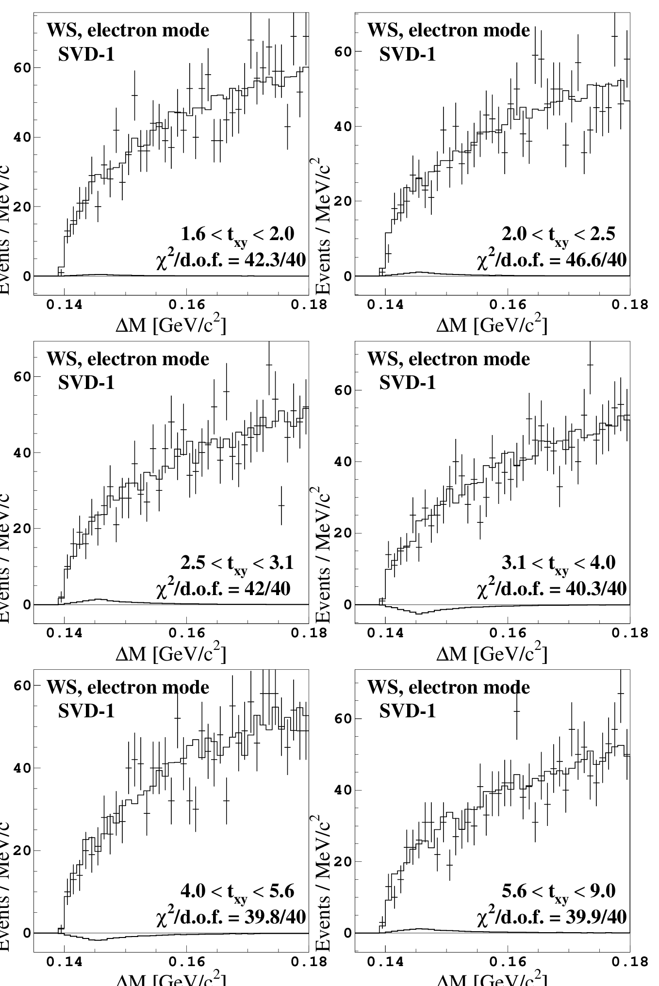
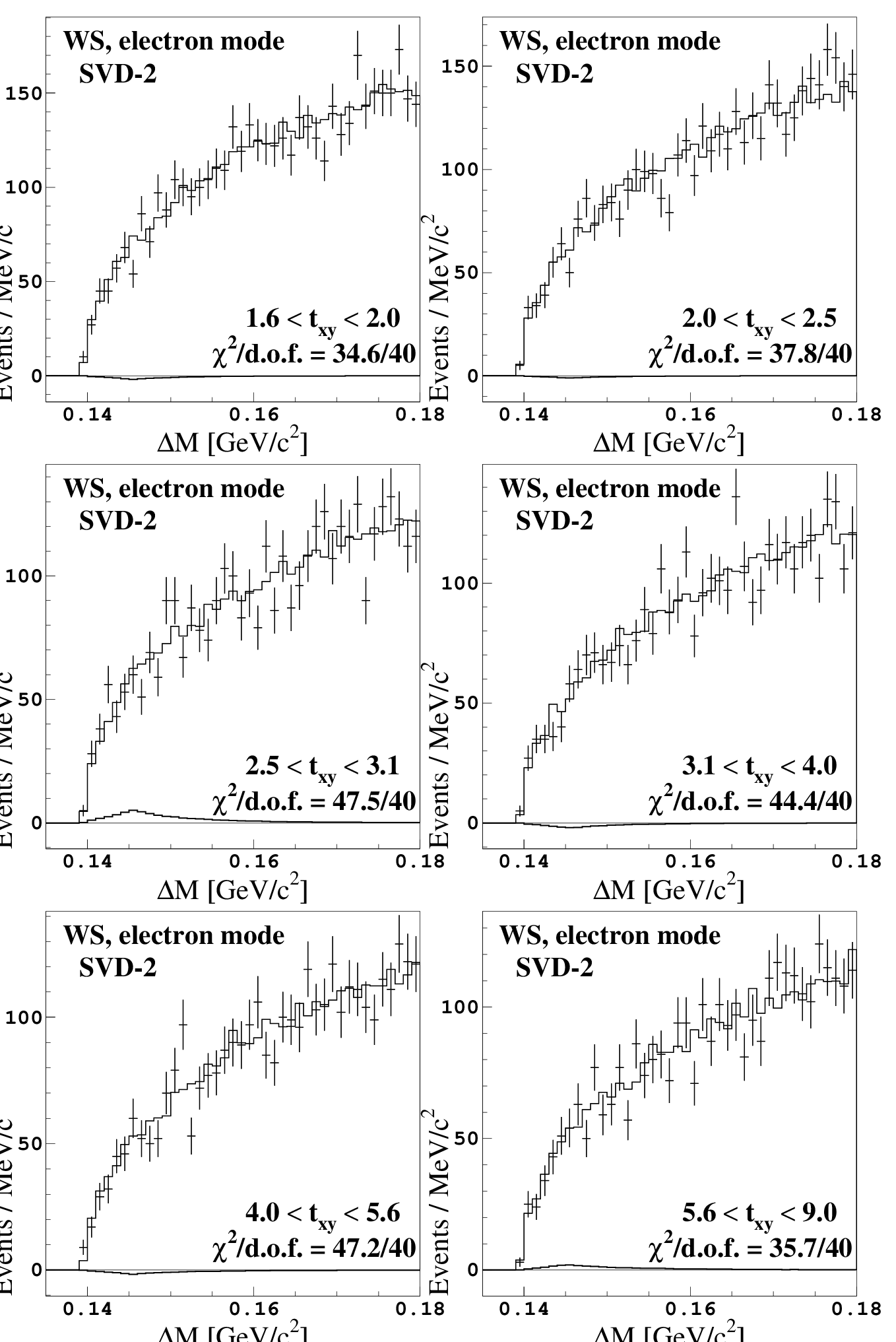
As the kinematic properties of the RS and WS decays are the same, we use the shape of the MC simulated RS signal events also for the WS signal decays. The distribution of the WS background events is obtained as described in Sec. IV.1. By fitting the distribution as described in Sec. IV.2, we extract the number of the mixed signal events in the four WS subsamples (e-1, e-2, -1, -2). The distributions and the values of the fits for all the subsamples and different proper decay time intervals are shown in Figs. 13, 14. The extracted WS signal yields are given in Table 7.
For each of the four subsamples we determine the mixing ratio by three different methods which are discussed below.
- 1)
The fit to in the RS and WS samples is performed without any selection based on the proper decay time measurement. The ratio is calculated as the ratio of the obtained number of WS and RS signal events, . The results can be found in Table 7 in rows labeled “all ”.
- 2)
The fit to distributions for the RS and WS sample is performed for events with . The ratio is calculated as . The results are given in Table 7 in rows labeled “1.6–9.0”. The resulting statistical uncertainty of the result is around 34% smaller than the one obtained by method 1).
- 3)
The third result, given in rows labeled “combined” of Table 7, is a fit of a constant to the six values measured in the six proper decay time bins. The six values and the result of the fit for each of the four subsamples are shown in Fig. 15. The statistical uncertainty of this result is 2–3% smaller than in method 2), because additional information on proper decay time is included through the six ratios.
Using the MC simulation, we verified that method 3) has the best sensitivity; we therefore quote as our final result the value obtained by method 3). To illustrate the effect of including the proper decay time information, we show also the results of methods 1) and 2).
From Table 7 one can see that the central values obtained by using the three methods, are slightly different. In evaluating the significance of the difference between the result of method 1) and the result of method 2), we have accounted for the ratio of the proper decay time efficiencies and for the statistical correlation between the samples. The differences are within the expected statistical fluctuations: they range between and standard deviations. By using toy MC simulation, it has also been verified that the differences in the central values between methods 2) and 3) are within the range of expected statistical fluctuations. For the default method 3), results for in all four subsamples are consistent with the null value. The values, shown in Fig. 15, are in good agreement with the expected distribution for 5 d.o.f., which has a maximum at the value of 3.0.
| e-1 subsample: | ||||||||
| 1.6–2.0 | 12578 | 94 | 4.8 | 27.2 | 0.915 | 0.007 | 3.5 | 19.8 |
| 2.0–2.5 | 11273 | 89 | 10.9 | 26.3 | 0.634 | 0.004 | 6.1 | 14.8 |
| 2.5–3.1 | 8975 | 84 | 14.7 | 25.6 | 0.443 | 0.002 | 7.2 | 12.6 |
| 3.1–4.0 | 7937 | 83 | –28.0 | 25.9 | 0.310 | 0.003 | –10.9 | 10.1 |
| 4.0–5.6 | 6394 | 85 | –21.2 | 28.6 | 0.223 | 0.003 | –7.4 | 10.0 |
| 5.6–9.0 | 4196 | 89 | 15.9 | 29.8 | 0.223 | 0.003 | 8.4 | 15.8 |
| combined | –1.7 | 5.2 | ||||||
| 1.6–9.0 | 51325 | 213 | –11.5 | 65.4 | 0.413 | 0.001 | –0.9 | 5.3 |
| all | 183496 | 443 | 70.1 | 141 | 1 | 3.8 | 7.7 | |
| e-2 subsample: | ||||||||
| 1.6–2.0 | 32616 | 150 | –19.1 | 44.0 | 0.881 | 0.003 | –5.2 | 11.9 |
| 2.0–2.5 | 28711 | 146 | –11.4 | 41.7 | 0.603 | 0.002 | –2.4 | 8.8 |
| 2.5–3.1 | 22513 | 131 | 52.5 | 41.9 | 0.415 | 0.002 | 9.7 | 7.7 |
| 3.1–4.0 | 18941 | 132 | –22.6 | 41.1 | 0.285 | 0.002 | –3.4 | 6.2 |
| 4.0–5.6 | 14796 | 129 | –18.6 | 42.3 | 0.198 | 0.002 | –2.5 | 5.7 |
| 5.6–9.0 | 9072 | 128 | 25.2 | 46.5 | 0.186 | 0.002 | 5.2 | 9.5 |
| combined | –0.1 | 3.1 | ||||||
| 1.6-9.0 | 126539 | 332 | –10.7 | 102 | 0.389 | 0.001 | –0.3 | 3.1 |
| all | 469947 | 701 | –369 | 222 | 1 | –7.8 | 4.7 | |
| -1 subsample: | ||||||||
| 1.6–2.0 | 11314 | 111 | 14.2 | 34.7 | 0.921 | 0.005 | 11.6 | 28.2 |
| 2.0–2.5 | 10185 | 109 | –1.8 | 33.5 | 0.637 | 0.004 | –1.1 | 21.0 |
| 2.5–3.1 | 7893 | 98 | 3.5 | 30.7 | 0.440 | 0.003 | 1.9 | 17.1 |
| 3.1–4.0 | 6804 | 96 | –5.5 | 31.8 | 0.303 | 0.002 | –2.5 | 14.2 |
| 4.0–5.6 | 5350 | 97 | 23.7 | 33.0 | 0.214 | 0.002 | 9.5 | 13.2 |
| 5.6–9.0 | 3670 | 90 | –12.8 | 35.4 | 0.217 | 0.003 | –7.6 | 20.9 |
| combined | 2.2 | 7.1 | ||||||
| 1.6–9.0 | 45181 | 245 | –11.2 | 79.9 | 0.410 | 0.001 | –1.0 | 7.2 |
| all | 163215 | 485 | –204 | 180 | 1 | –12.5 | 11.0 | |
| -2 subsample: | ||||||||
| 1.6–2.0 | 27612 | 180 | 71.4 | 54.8 | 0.876 | 0.015 | 22.7 | 17.4 |
| 2.0–2.5 | 23695 | 170 | 9.3 | 52.3 | 0.595 | 0.010 | 2.3 | 13.1 |
| 2.5–3.1 | 18905 | 154 | 82.3 | 49.8 | 0.405 | 0.006 | 17.6 | 10.7 |
| 3.1–4.0 | 15488 | 150 | 51.1 | 50.1 | 0.273 | 0.004 | 9.0 | 8.8 |
| 4.0–5.6 | 11989 | 144 | 20.4 | 51.1 | 0.186 | 0.007 | 3.2 | 7.9 |
| 5.6–9.0 | 7146 | 138 | –20.3 | 56.5 | 0.171 | 0.016 | –4.9 | 13.6 |
| combined | 7.4 | 4.4 | ||||||
| 1.6–9.0 | 104556 | 381 | 192 | 125 | 0.380 | 0.002 | 7.0 | 4.5 |
| all | 396151 | 761 | 170 | 284 | 1 | 4.3 | 7.2 | |
The combined result for the electron decay mode is obtained by a fit to the values for the e-1 and e-2 subsamples, obtained by method 3). The fit yields with a value of 0.1 per 1 degree of freedom. The combined result for the muon decay mode is obtained in the same way; the fit yields with a value of 0.4.
The combined result, taking into account the statistical uncertainty only, is obtained by a fit to the four values (electron and muon decay mode, SVD-1 and SVD-2); it yields a value of
| (22) |
where the quoted uncertainty is statistical only. The value is 2.5 for three degrees of freedom. The values for the four subsamples and the result of the fit are shown in the left plot of Fig. 16. To obtain the final result, the partially correlated systematic uncertainties have to be studied and taken into account.


V.1 Systematic uncertainties
In the following subsection, different sources of the systematic uncertainties are discussed and the systematic uncertainties are given; they are summarized in Table 8.
V.1.1 Finite statistics of the fitting distributions
One of the main sources of systematic uncertainty is the limited statistics of the samples used to obtain the signal and background distributions used in the fit to data. To estimate this, we vary the contents of all bins of the RS and WS, signal and background distributions independently in accordance with each bin’s statistical uncertainty. We repeat the fit to the RS and WS data, calculate the corresponding in each proper decay time interval, and obtain a new value. Repeating the procedure 1000 times, the obtained distribution of values has a Gaussian shape. The sigma of the Gaussian, fitted to the distribution, is taken as the systematic uncertainty due to the limited statistics of the fitting distributions. The uncertainties are listed in Table 8, line 1. Larger uncertainties in the muon decay mode reflect the fact that, compared to the electron decay mode, the muon background is larger especially in the signal region, and secondly, the embedded slow pion sample is smaller due to the smaller value used. Since this uncertainty is statistical in nature, it is considered to be completely uncorrelated between the four subsamples (e-1, e-2, -1, -2).
V.1.2 The amount of WS correlated background
The normalization of the WS-correlated background is determined by MC simulation, taking into account the central values of branching fractions [23], of decay modes that contribute to this background.
From MC simulation studies we find that in the electron decay mode the largest contributions to the WS correlated background come from the following decays: ( mesons mainly from decays, 34% of the correlated background), (12%), (7%), (7%). In total 60% of the correlated background comes from these decays.
In the muon decay mode, the largest contributions to the WS correlated background come from (19%), (12%), (7%), (7%), (4%), (4%). In total 53% of the correlated background comes from these decays. We calculate the weighted average of the relative uncertainties of the branching fractions [23] for the stated decay modes. For the electron decay mode, the averaged relative uncertainty is 3.6% and for the muon decay mode 5.9%. To take into account the uncertainties of the branching fractions used in the MC simulation, we repeat the WS fits, changing the amount of the total WS correlated background by the average uncertainties on the branching fractions. The differences between the resulting values and the default values are taken as the systematic uncertainty from this source; they are listed in Table 8, line 2.
This procedure is conservative for two reasons. First, by varying the total correlated background instead of varying its individual components, the uncertainties on the branching fractions are implicitly considered to be 100% correlated, resulting in the maximum possible systematic uncertainty. Second, the modes comprising the correlated background contribute significantly also to the uncorrelated background. Taking this into account would lead to a smaller change in .
This uncertainty is larger in the muon decay mode, because the probabilities to misidentify a pion or kaon as a muon are much larger than the corresponding probabilities for misidentification as an electron. Consequently, in the muon decay mode the fraction of the correlated background is significantly larger (Table 5), its shape tends to lower values (Fig. 11) and its averaged uncertainty of the branching fractions is larger.
The systematic uncertainty from this source is the same for the SVD-1 and SVD-2 subsample. Since a significant part of the correlated background is due to decays common to the electron and the muon decay modes, the systematic uncertainties for both decay modes are highly correlated. Hence the systematic uncertainty from this source will be treated as 100% correlated for all four subsamples (e-1, e-2, -1, -2).
V.1.3 The shape of the WS uncorrelated background
We also conservatively account for the uncertainty of the shape of the WS uncorrelated background. We vary within the limits given by the statistical uncertainties of the values in Table 6. The statistical uncertainty for the data is in the electron decay mode and in the muon decay mode. For the embedded slow pion sample, the value changes by 0.1 for . Hence is varied by in the electron decay mode, and by in the muon decay mode. With the new distributions we repeat the fit to WS data, recalculate the values and quote the differences from the default values as the systematic uncertainties from this source. These uncertainties are listed on line 3 of Table 8.
Since is determined for the electron and muon decay mode separately and the uncertainty on is statistical in nature, this systematic uncertainty is considered to be completely uncorrelated between both decay modes. On the other hand, is determined for SVD-1 and SVD-2 subsamples together, hence the uncertainty is treated as completely correlated between them.
V.1.4 Proper decay time distribution
To check the reliability of efficiencies and ratios , and to estimate the effect of the imperfect fit to the proper decay time distribution, the values of are compared to an alternative estimate from the fit to , . This method accounts for the influence of the associated signal in the distribution. In a majority of the subintervals, and typically agree within , the largest discrepancies being and . For the integrated interval, they agree within 0.8%–1.4% for the four subsamples.
To estimate the effect of the discrepancies, the relative difference between and is assigned as the relative uncertainty on . Hence we reduce the six effciency ratios simultaneously by this uncertainty and repeat the calculation; we then increase the ratios by this uncertainty, and again recalculate . The difference between the resulting value and the default fit is quoted as the systematic uncertainty from this source. It is very small and can be found on line 4 of Table 8.


V.1.5 The amount of the associated signal
The systematic error due to the uncertainty in the associated signal fraction is estimated by varying the fraction and repeating the fitting procedure. Taking into account the uncertainties on the measured branching fractions [23] of the associated signal decay channels, we conservatively vary the amount of associated signal by . We recalculate the values and compare them to the default value; we quote the differences as the systematic uncertainty from this source. From Table 8 (line 5) one can see that it is almost negligible.


V.1.6 The amount of the RS correlated background
From MC simulation studies we find that in the electron decay mode the largest contributions to the RS correlated background come from the following decays: (33% of the RS correlated background), (14%), (13%). In total 60% of the RS correlated background comes from these three decays.
In the muon decay mode, the largest contributions to the RS correlated background come from (43%), (17%), (12%). In total 72% of the correlated background comes from these decays. We calculate the weighted average of the relative uncertainties of the branching fractions [23] for the stated decay modes. For the electron decay mode the averaged relative uncertainty is 4.3% and for the muon decay mode 4.4%.
We repeat the RS fits, changing the amount of the total correlated background by the average uncertainties on the branching fractions. The differences between the obtained values of and the default values are taken as the systematic uncertainty from this source. They can be found in Table 8 (line 6) and are negligible.
| source | e-1 | e-2 | -1 | -2 | |
|---|---|---|---|---|---|
| 1 | fitting histo. statistics | 1.54 | 0.91 | 2.64 | 1.81 |
| 2 | WS correlated bkg. | 0.37 | |||
| 3 | WS uncorrelated bkg. | ||||
| 4 | imperfect | 0.05 | 0.02 | 0.01 | |
| 5 | associated signal | 0.00 | 0.02 | ||
| 6 | RS correlated bkg. | 0.00 | 0.00 | 0.01 | 0.04 |
| total systematic | |||||
| statistical + systematic |
V.1.7 Total systematic uncertainty and the final result
The final result of the measurement is obtained by averaging the results for the four subsamples, e-1, e-2, and . As explained at the beginning of Sec. V, the results obtained by method 3) are used (quoted in Table 7) as “combined”.
The contributions to the systematic uncertainty are divided into three categories:
- (a)
The systematic uncertainty that is completely correlated between all four subsamples. This is the error due to the uncertainty of the WS correlated background fraction, Sec. V.1.2.
- (b)
The systematic uncertainty that is completely correlated between the SVD-1 and SVD-2 subsamples and is uncorrelated between the electron and the muon decay mode. Such a contribution comes from the uncertainty of the shape of the uncorrelated WS background, Sec. V.1.3.
- (c)
The systematic uncertainties that are uncorrelated between the four subsamples, or are very small. The main contribution comes from the uncertainty due to the finite statistics of the fitting distributions, Sec. V.1.1. The uncertainties from all the remaining sources are also added.
To obtain the final result and its uncertainty, taking into account the systematic uncertainties, we adopt the following procedure:
- (1)
For each of the four subsamples, we add to the statistical uncertainty in quadrature all the uncertainties from category (c).
- (2)
We perform the fit to the SVD-1 and SVD-2 values in the electron and muon decay mode to obtain the averaged value for the electron and muon decay mode, and , respectively. The quoted uncertainties include the statistical uncertainty and the uncertainties (c).
- (3)
To add the uncertainty (b) for the electron decay mode, we first simultaneously increase and then simultaneously decrease the results for the e-1 and e-2 subsamples by the uncertainty (b) and repeat step (2). The difference from the default result of step (2) is added in quadrature to the uncertainty obtained in step (2). The result for the electron decay mode, including the statistical uncertainty and systematic uncertainties (b) and (c), is . We perform the same procedure also for the muon decay mode; the result is .
- (4)
We perform a fit to the results for the electron and muon decay mode, obtained in step (3); the result is . The obtained mean value is the final result, but the uncertainty needs to be increased by the uncertainty (a).
- (5)
To account for the uncertainty (a) we first simultaneously increase and then simultaneously decrease the initial four values by the uncertainties (a) and repeat the steps (1)–(4). The difference from the default result, , is added in quadrature to the uncertainty previously obtained from step (4) to obtain the final uncertainty of the result.
The total uncertainty of the final result is . We calculate the contribution of the systematic uncertainty as the difference between the total uncertainty and the statistical uncertainty (Eq. (22)), . The final result is then
| (23) |
where the first uncertainty is statistical and the second systematic. As this value is close to the boundary of the physical region () we use the Feldman-Cousins approach [26] to calculate upper limits:
| (24) | |||
| (25) |
With systematic uncertainties included, the final results for the electron and muon decay modes are:
| (26) | |||
| (27) |
The values for the four subsamples, including the systematic uncertainty, and the combined result are shown in the right plot in Fig. 16.
The increase in the sensitivity of the current result, compared to the one published in [7], is caused partially by the larger statistical power of the sample, but also by the improvements in the measurement method. The statistical uncertainty of the present result in the electron sample (Eq. (26)) is about 22% smaller than one would expect by appropriately rescaling the uncertainty of the result [7] by the increase of the data set used. The improvement is mainly due to improved selection criteria, improved neutrino reconstruction and improvements in using the proper decay time measurement. The systematic error of the result in the electron sample is, however, larger than the one published in [7] as it is estimated more conservatively.
VI SUMMARY
Using a data sample with an integrated luminosity of 492.2 fb-1, collected by the Belle detector, we have searched for - mixing using semileptonic decays of the neutral charmed meson, and We select mesons produced via the decay , and tag the flavor of the meson at production by the charge of the accompanying slow pion. The measured mixing rate is consistent with no mixing in both electron and muon decay modes. The combined result accounts for the partially correlated systematic error and yields . Since it is consistent with zero we set upper limits on the mixing rate of at the 90% confidence level.
This result supersedes that published in Ref. [7] and represents the most stringent experimental limit on obtained to date from semileptonic decays. Its accuracy is significantly better than that of the world average of previous measurements in semileptonic decays, [4]. Although the sensitivity is not sufficient to observe a positive mixing signal, it is worth noting that in semileptonic decays no model uncertainties can influence the result. The reported value of is in agreement with the world average values of and [4] and it will help in further constraining the mixing parameters in combination with the results of the measurements in other decay channels.
Appendix
In the proper decay time fit the following functions are used:
The Lorentz function, centered at 0:
| (28) |
The asymmetric Lorentz function, centered at 0:
Acknowledgements.
We thank the KEKB group for the excellent operation of the accelerator, the KEK cryogenics group for the efficient operation of the solenoid, and the KEK computer group and the National Institute of Informatics for valuable computing and Super-SINET network support. We acknowledge support from the Ministry of Education, Culture, Sports, Science, and Technology of Japan and the Japan Society for the Promotion of Science; the Australian Research Council and the Australian Department of Education, Science and Training; the National Natural Science Foundation of China under contract No. 10575109 and 10775142; the Department of Science and Technology of India; the BK21 program of the Ministry of Education of Korea, the CHEP SRC program and Basic Research program (grant No. R01-2005-000-10089-0) of the Korea Science and Engineering Foundation, and the Pure Basic Research Group program of the Korea Research Foundation; the Polish State Committee for Scientific Research; the Ministry of Education and Science of the Russian Federation and the Russian Federal Agency for Atomic Energy; the Slovenian Research Agency; the Swiss National Science Foundation; the National Science Council and the Ministry of Education of Taiwan; and the U.S. Department of Energy.References
- [1] M. Starič et al. (Belle Collaboration), Phys. Rev. Lett. 98 211803 (2007).
- [2] B. Aubert et al., (BaBar Collaboration), Phys. Rev. Lett. 98, 211802 (2007).
- [3] See the talks by W. Lockman (http://chep.knu.ac.kr/ lp07/htm/S4/S04_13a.pdf) and K. Tollefson (http:// chep.knu.ac.kr/lp07/htm/S4/S04_14.pdf) at Lepton Photon 2007; W. M. Sun (for CLEO), arXiv:0712.0498v1.
- [4] Heavy Flavor Averaging Group (Charm Decays subgroup), http://www.slac.stanford.edu/xorg/hfag/ charm/index.html
- [5] For a review see I.I. Bigi and N. Uraltsev, Nucl. Phys. B 592, 92 (2001); S. Bianco, F.L. Fabbri, D. Benson and I. Bigi, Riv. Nuovo Cim. 26N7, 1 (2003); A. Falk et al., Phys. Rev D 69, 114021 (2004).
- [6] Z.-Z. Xing, Phys. Rev. D 55, 196 (1997).
- [7] U. Bitenc et al. (Belle Collaboration), Phys. Rev. D 72, 071101 (2005).
- [8] B. Aubert et al. (BaBar Collaboration), Phys. Rev. D 70, 091102 (2004); B. Aubert et al. (BaBar Collaboration), Phys. Rev. D 76, 014018 (2007) .
- [9] C. Cawlfield et al. (CLEO Collaboration), Phys. Rev. D 71, 077101 (2005).
- [10] E. M. Aitala et al. (E791 Collaboration), Phys. Rev. Lett. 77, 2384 (1996).
- [11] L. Zhang et al. (Belle Collaboration), Phys. Rev. Lett. 96, 151801 (2006).
- [12] B. Aubert et al. (BaBar Collaboration), Phys. Rev. Lett. 97, 221803 (2006).
- [13] B. Aubert et al. (BaBar Collaboration), hep-ex/0607090.
- [14] S. Kurokawa and E. Kikutani, Nucl. Instr. Meth. A 499, 1 (2003), and other papers included in this volume.
- [15] A. Abashian et al. (Belle Collaboration), Nucl. Instr. Meth. A 479, 117 (2002).
- [16] Z. Natkaniec et al. (Belle SVD-2 group), Nucl. Instr. Meth. A 560, 1 (2006).
- [17] Events are simulated with the EvtGen generator, D.-J. Lange, Nucl. Instr. Methods Phys. Res., Sect. A 462, 152 (2001); the detector response is simulated with GEANT, R. Brun et al., GEANT 3.21, CERN Report No. DD/EE/84-1, 1984.
- [18] The charge-conjugate modes are implied throughout the paper unless otherwise stated.
- [19] K. Abe et al. (Belle Collaboration), Phys. Rev. D 66 032007 (2002).
- [20] G. C. Fox, S. Wolfram, Phys. Rev. Lett. 41, 1581 (1978).
- [21] K. Hanagaki et al., Nucl. Instr. Meth. A 485, 490 (2002).
- [22] A. Abashian et al., Nucl. Instr. Meth. A 491, 69 (2002).
- [23] W.-M. Yao et al. (Particle Data Group), J. Phys. G 33, 1 (2006).
- [24] In the following, denotes the particle’s 4-momentum while and denote the 3-dimensional momentum and its magnitude, respectively.
- [25] The actual mass assignment of tracks included in has only a marginal effect on the neutrino reconstruction and thus on the resolution. If all charged particles are assigned a mass of the pion the resolution remains almost the same.
- [26] G.J. Feldman and R.D. Cousins, Phys. Rev. D 57, 3873 (1998).