Classification Constrained Dimensionality Reduction

Raviv Raich Jose A. Costa Steven B. Damelin and Alfred O. Hero III ^†^†thanks: This work was partially funded by the DARPA Defense Sciences Office under Office of Naval Research contract #N00014-04-C-0437. Distribution Statement A. Approved for public release; distribution is unlimited. S. B. Damelin was supported in part by National Science Foundation grant no. NSF-DMS-0555839 and NSF-DMS-0439734 and by AFRL. ^†^†thanks: R. Raich is with the Oregon State University, Corvallis. A. O Hero III is with the University of Michigan, Ann Arbor. J. A. Costa is with the California Institute of Technology. S. B. Damelin is with the Georgia Southern University.

Abstract

Dimensionality reduction is a topic of recent interest. In this paper, we present the classification constrained dimensionality reduction (CCDR) algorithm to account for label information. The algorithm can account for multiple classes as well as the semi-supervised setting. We present an out-of-sample expressions for both labeled and unlabeled data. For unlabeled data, we introduce a method of embedding a new point as preprocessing to a classifier. For labeled data, we introduce a method that improves the embedding during the training phase using the out-of-sample extension. We investigate classification performance using the CCDR algorithm on hyper-spectral satellite imagery data. We demonstrate the performance gain for both local and global classifiers and demonstrate a $10\%$ improvement of the $k$ -nearest neighbors algorithm performance. We present a connection between intrinsic dimension estimation and the optimal embedding dimension obtained using the CCDR algorithm.

Index Terms:

Classification, Computational Complexity, Dimensionality Reduction, Embedding, High Dimensional Data, Kernel, K-Nearest Neighbor, Manifold Learning, Probability, Out-of-Sample Extension.

I Introduction

In classification theory, the main goal is to find a mapping from an observation space ${\cal X}$ consisting of a collection of points in some containing Euclidean space $\mathds{R}^{d}$ , $d\geq 1$ into a set consisting of several different integer valued hypotheses. In some problems, the observations from the set ${\cal X}$ lie on a $d$ -dimensional manifold $\mathcal{M}$ and Whitney’s theorem tells us that provided that this manifold is smooth enough, there exists an embedding of $\mathcal{M}$ into $\mathds{R}^{2d+1}$ . This motivates the approach taken by kernel methods in classification theory, such as support vector machines [1] for example. Our interest is in finding an embedding of $\mathcal{M}$ into a lower dimensional Euclidean space.

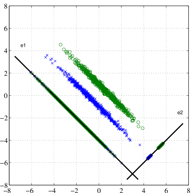
Refer to caption — Fig. 1: PCA of a two-classes classification problem.

Dimensionality reduction of high dimensional data, was addressed in classical methods such as principal component analysis (PCA) [2] and multidimensional scaling (MDS) [3, 4]. In PCA, an eigendecomposition of the $d\times d$ empirical covariance matrix is performed and the data points are linearly projected along the $0<m\leq d$ eigenvectors with the largest eigenvalues. A problem that may occur with PCA for classification is demonstrated in Fig. 1. When the information that is relevant for classification is present only in the eigenvectors associated with the small eigenvalues ( $e_{2}$ in the figure), removal of such eigenvectors may result in severe degradation in classification performance. In MDS, the goal is to find a lower dimensional embedding of the original data points that preserves the relative distances between all the data points. The two later methods suffer greatly when the manifold is nonlinear. For example, PCA will not be able to offer dimensionality reduction for classification of two classes lying each on one of two concentric circles.

In [5], a nonlinear extension to PCA is presented. The algorithm is based on the “kernel trick” [6]. Data points are nonlinearly mapped into a feature space, which in general has a higher (or even infinite) dimension as compared with the original space and then PCA is applied to the high dimensional data.

In the paper of Tenenbaum et al [7], Isomap, a global dimensionality reduction algorithm was introduced taking into account the fact that data points may lie on a lower dimensional manifold. Unlike MDS, geodesic distances (distances that are measured along the manifold) are preserved by Isomap. Isomap utilizes the classical MDS algorithm, but instead of using the matrix of Euclidean distances, it uses a modified version of it. Each point is connected only to points in its local neighborhood. A distance between a point and another point outside its local neighborhood is replaced with the sum of distances along the shortest path in graph. This procedure modifies the squared distances matrix replacing Euclidian with geodesic distances.

In [8], Belkin and Niyogi present a related Laplacian eigenmap dimensionality reduction algorithm. The algorithm performs a minimization on the weighted sum of squared-distances of the lower-dimensional data. Each weight multiplying the squared-distances of two low-dimensional data points is inversely related to distance between the corresponding two high-dimensional data points. Therefore, small distance between two high-dimensional data points results in small distance between two low-dimensional data points. To preserve the geodesic distances, the weight of the distance between two points that do not share a local neighborhood is set to zero.

We refer the interested reader to the references below and those cited therein for a list of some of the most commonly used additional algorithms within the class of manifold learning algorithms and their different advantages relevent to our work. Locally Linear Embedding (LLE) [9], Laplacian Eigenmaps [8], Hessian Eigenmaps (HLLE) [10], Local Space Tangent Analysis [11], Diffusion Maps [12] and Semidefinite Embedding (SDE)[13].

The algorithms mentioned above, consider the problem of learning a lower-dimensional embedding of the data. In classification, such algorithms can be used to preprocess high-dimensional data before performing the classification. This could potentially allow for a lower computational complexity of the classifier. In some cases, dimensionality reduction results increase the computational complexity of the classifier. In fact, support vector machines suggest the opposing strategy: data points are projected onto a higher-dimensional space and classified by a low computational complexity classifier. To guarantee a low computational complexity of the classifier of the low-dimensional data, a classification constrained dimensionality reduction (CCDR) algorithm was introduced in [14]. The CCDR algorithm is an extension of Laplacian eigenmaps [8] and it incorporates class label information into the cost function, reducing the distance between points with similar label. Another algorithm that incorporates label information is the marginal fisher analysis (MFA) [15], in which a constraint on the margin between classes is used to enforce class separation.

In [14] the CCDR algorithm was only studied for two classes and its performance was illustrated for simulated data. In [16], a multi-class extension to the problem was presented. In this paper, we introduce two additional components that make the algorithm computationally viable. The first is an out-of-sample extension for classification of unlabeled test points. Similarly to the out-of-sample extension presented in [17], one can utilize the Nyström formula for classification problems in which label information is available. We study the algorithm performance as its various parameters, (e.g., dimension, label importance, and local neighborhood), are varied. We study the performance of CCDR as preprocessing prior to implementation of several classification algorithms such as $k$ -nearest neighbors, linear classification, and neural networks. We demonstrate a $10\%$ improvement over the $k$ -nearest neighbors algorithm performance benchmark for this dataset. We address the issue of dimension estimation and its effect on classification performance.

The organization of this paper is as follows. Section III presents the multiple-class CCDR algorithm. Section provides a study of the algorithm using the Landsat dataset and Section VI summaries our results.

II Dimensionality Reduction

Let $\mathcal{X}_{n}=\{\mbox{\boldmath$x$}_{1},\mbox{\boldmath$x$}_{2},\ldots,\mbox{\boldmath$x$}_{n}\}$ be a set of $n$ points constrained to lie on an $m$ -dimensional submanifold $\mathcal{M}\subseteq\mathds{R}^{d}$ . In dimensionality reduction, our goal is to obtain a lower-dimensional embedding $\mathcal{Y}_{n}=\{\mbox{\boldmath$y$}_{1},\mbox{\boldmath$y$}_{2},\ldots,\mbox{\boldmath$y$}_{n}\}$ (where $\mbox{\boldmath$y$}_{i}\in\mathds{R}^{m}$ with $m<d$ ) that preserves local geometry information such that processing of the lower dimensional embedding $\mathcal{Y}_{n}$ yields comparable performance to processing of the original data points $\mathcal{X}_{n}$ . Alternatively, we would like learn the mapping $f:\mathcal{M}\subseteq\mathds{R}^{d}\to\mathds{R}^{m}$ that maps every data point $\mbox{\boldmath$x$}_{i}$ to $\mbox{\boldmath$y$}_{i}=f(\mbox{\boldmath$x$}_{i})$ such that some geometric properties of the high-dimensional data are preserved in the lower dimensional embedding. The first question that comes to mind is how to select $f$ , or more specifically how to restrict the function $f$ so that we can still achieve our goal.

II-A Linear dimensionality reduction

II-A1 PCA

When principal component analysis (PCA) is used for dimensionality reduction, one considers a linear embedding of the form

\displaystyle\mbox{\boldmath$y$}_{i}=f(\mbox{\boldmath$x$}_{i})={\bm{A}}\mbox{\boldmath$x$}_{i},

where ${\bm{A}}$ is $m\times d$ . This embedding captures the notion of proximity in the sense that close points in the high dimensional space map to close points in the lower dimensional embedding, i.e., $\|\mbox{\boldmath$y$}_{i}-\mbox{\boldmath$y$}_{j}\|=\|{\bm{A}}(\mbox{\boldmath$x$}_{i}-\mbox{\boldmath$x$}_{j})\|\leq\|{\bm{A}}\|\|\mbox{\boldmath$x$}_{i}-\mbox{\boldmath$x$}_{j}\|$ . Let

\bar{\mbox{\boldmath$x$}}=\frac{1}{n}\sum_{i=1}^{n}\mbox{\boldmath$x$}_{i}

and

\mathcal{C}_{x}=\frac{1}{n}\sum_{i=1}^{n}(\mbox{\boldmath$x$}_{i}-\bar{\mbox{\boldmath$x$}})(\mbox{\boldmath$x$}_{i}-\bar{\mbox{\boldmath$x$}})^{T}.

Similarly, let

\bar{\mbox{\boldmath$y$}}=\frac{1}{n}\sum_{i=1}^{n}\mbox{\boldmath$y$}_{i}

and

\mathcal{C}_{y}=\frac{1}{n}\sum_{i=1}^{n}(\mbox{\boldmath$y$}_{i}-\bar{\mbox{\boldmath$y$}})(\mbox{\boldmath$y$}_{i}-\bar{\mbox{\boldmath$y$}})^{T}.

Since $\mbox{\boldmath$y$}_{i}={\bm{A}}\mbox{\boldmath$x$}_{i}$ , we have $\bar{\mbox{\boldmath$y$}}={\bm{A}}\bar{\mbox{\boldmath$x$}}$ and $\mathcal{C}_{y}={\bm{A}}\mathcal{C}_{x}{\bm{A}}^{T}$ . In PCA, the goal is to find the projection matrix ${\bm{A}}$ that preserves most of the energy in the original data by solving

\displaystyle\max_{{\bm{A}}}\mbox{tr}\{\mathcal{C}_{y}({\bm{A}})\}\quad\textrm{s.t.}\quad{\bm{A}}{\bm{A}}^{T}={\bm{I}},

which is equivalent to

\displaystyle\max_{{\bm{A}}}\mbox{tr}\{{\bm{A}}\mathcal{C}_{x}{\bm{A}}^{T}\}\quad\textrm{s.t.}\quad{\bm{A}}{\bm{A}}^{T}={\bm{I}}.

(1)

The solution to (1), is given by ${\bm{A}}=[{\bf u}_{1},{\bf u}_{2},\ldots,{\bf u}_{m}]^{T}$ , where ${\bf u}_{i}$ is the eigenvector of $\mathcal{C}_{x}$ corresponding to its $i$ th largest eigenvalue. When the data lies on an $m$ -dimensional hyperplane, the matrix $\mathcal{C}_{x}$ has only $m$ positive eigenvalues and the rest are zero. Furthermore, every $\mbox{\boldmath$x$}_{i}$ belongs to $\bar{\mbox{\boldmath$x$}}+\textrm{span}\{{\bf u}_{1},{\bf u}_{2},\ldots,{\bf u}_{m}\}\subseteq\mathds{R}^{d}$ . In this case, the mapping PCA finds $f(\mbox{\boldmath$x$})={\bm{A}}\mbox{\boldmath$x$}$ is one-to-one and satisfies $\|f(\mbox{\boldmath$x$}_{i})-f(\mbox{\boldmath$x$}_{j})\|=\|{\bm{A}}(\mbox{\boldmath$x$}_{i}-\mbox{\boldmath$x$}_{j})\|=\|\mbox{\boldmath$x$}_{i}-\mbox{\boldmath$x$}_{j}\|$ . Therefore, the lower embedding preserves all the geometry information in the original dataset $\mathcal{X}$ . We would like to point out that PCA can be written as

\displaystyle\max_{\{\mathcal{Y}\}}\sum_{i=1}^{n}\|\mbox{\boldmath$y$}_{i}-\mbox{\boldmath$y$}_{j}\|^{2}\quad\textrm{s.t.}\quad\mbox{\boldmath$y$}_{i}={\bm{A}}\mbox{\boldmath$x$}_{i}~\textrm{and}~{\bm{A}}{\bm{A}}^{T}={\bm{I}},

II-A2 MDS

Multidimensional Scaling (MDS) differs from PCA in the way the input is provided to it. While in PCA, the original data $\mathcal{X}$ is provided, the classical MDS requires only the set of all Euclidean pairwise distances $\{\|\mbox{\boldmath$x$}_{i}-\mbox{\boldmath$x$}_{j}\|_{2}\}_{i=1,j>i}^{n-1}$ . As MDS uses only pairwise distances, the solution it finds is given up to translation and unitary transformation. Let $\mbox{\boldmath$x$}^{\prime}_{i}=\mbox{\boldmath$x$}_{i}-{\bf c}$ , the Euclidean distance $\|\mbox{\boldmath$x$}^{\prime}_{i}-\mbox{\boldmath$x$}^{\prime}_{j}\|$ is the same as $\|\mbox{\boldmath$x$}_{i}-\mbox{\boldmath$x$}_{j}\|$ . Let $U$ be an arbitrary unitary matrix $U$ satisfying $\mbox{\boldmath$U$}^{T}\mbox{\boldmath$U$}={\bm{I}}$ and define $\mbox{\boldmath$x$}^{\prime}_{i}=\mbox{\boldmath$U$}\mbox{\boldmath$x$}$ . The distance $\|\mbox{\boldmath$x$}^{\prime}_{i}-\mbox{\boldmath$x$}^{\prime}_{j}\|$ is equal to $\|\mbox{\boldmath$U$}(\mbox{\boldmath$x$}_{i}-\mbox{\boldmath$x$}_{j})\|$ , which by the invariance of the Euclidean norm to a unitary transformation equals to $\|\mbox{\boldmath$x$}_{i}-\mbox{\boldmath$x$}_{j}\|$ . Denote the pairwise squared-distance matrix by $[\mbox{\boldmath$D$}_{2}]_{ij}=\|\mbox{\boldmath$x$}_{i}-\mbox{\boldmath$x$}_{j}\|^{2}$ . By the definition of Euclidean distance, the matrix $\mbox{\boldmath$D$}_{2}$ satisfies

\displaystyle\mbox{\boldmath$D$}_{2}={\bf 1}\mbox{\boldmath$\phi$}^{T}+\mbox{\boldmath$\phi$}{\bf 1}^{T}-2\mbox{\boldmath$X$}^{T}\mbox{\boldmath$X$},

(2)

where $\mbox{\boldmath$X$}=[\mbox{\boldmath$x$}_{1},\mbox{\boldmath$x$}_{2},\ldots,\mbox{\boldmath$x$}_{n}]$ and $\mbox{\boldmath$\phi$}=[\|\mbox{\boldmath$x$}_{1}\|^{2},\|\mbox{\boldmath$x$}_{2}\|^{2},\ldots,\|\mbox{\boldmath$x$}_{n}\|^{2}]^{T}$ . To verify (2), one can examine the $ij$ -th term of $\mbox{\boldmath$D$}_{2}$ and compare with $\|\mbox{\boldmath$x$}_{i}-\mbox{\boldmath$x$}_{j}\|^{2}$ . Denote the $n\times n$ matrix $\mbox{\boldmath$H$}={\bm{I}}-{\bf 1}{\bf 1}^{T}/n$ . Multiplying both sides of $\mbox{\boldmath$D$}_{2}$ with $H$ in addition to a factor of $-\frac{1}{2}$ , yields

-\frac{1}{2}\mbox{\boldmath$H$}\mbox{\boldmath$D$}_{2}\mbox{\boldmath$H$}=(\mbox{\boldmath$X$}\mbox{\boldmath$H$})^{T}(\mbox{\boldmath$X$}\mbox{\boldmath$H$}),

which is key to MDS, i.e., Cholesky decomposition of $-\frac{1}{2}\mbox{\boldmath$H$}\mbox{\boldmath$D$}_{2}\mbox{\boldmath$H$}$ yields $X$ to within a translation and a unitary transformation. Consider the eigendecomposition $-\frac{1}{2}\mbox{\boldmath$H$}\mbox{\boldmath$D$}_{2}\mbox{\boldmath$H$}=\mbox{\boldmath$U$}{\bm{\Lambda}}\mbox{\boldmath$U$}^{T}$ . Therefore, a rank $d$ $X$ can be obtained as $\mbox{\boldmath$X$}={\bm{\Lambda}}_{d}^{\frac{1}{2}}\mbox{\boldmath$U$}_{d}^{T}$ , where ${\bm{\Lambda}}_{d}={\rm diag}\{[\lambda_{1},\lambda_{2},\ldots,\lambda_{d}]\}^{\frac{1}{2}}$ and $\mbox{\boldmath$U$}_{d}=[{\bf u}_{1},{\bf u}_{2},\ldots,{\bf u}_{d}]$ . Note that $X$ $H$ is a translated version of $X$ , in which every column $\mbox{\boldmath$x$}_{i}$ is translated to $\mbox{\boldmath$x$}_{i}-\bar{\mbox{\boldmath$x$}}$ .

To use MDS for dimensionality reduction, we can consider a two step process. First a square-distance matrix $\mbox{\boldmath$D$}_{2}$ is obtained from the high-dimensional data $\mathcal{X}$ . Then, MDS is applied to $\mbox{\boldmath$D$}_{2}$ to obtain a low-dimensional ( $m<d$ ) embedding by $\mbox{\boldmath$X$}_{m}={\bm{\Lambda}}_{m}^{\frac{1}{2}}\mbox{\boldmath$U$}_{m}^{T}=\mbox{\boldmath$X$}\mbox{\boldmath$U$}_{m}\mbox{\boldmath$U$}_{m}^{T}$ . In the absence of noise, this procedure provides an affine transformation to the high-dimensional data and thus can be regarded as a linear method.

II-B Nonlinear dimensionality reduction

Linear maps are limited as they cannot preserve the geometry of nonlinear manifolds.

II-B1 Kernel PCA

Kernel PCA is one of the first methods in dimensionality reduction of data on nonlinear manifolds. The method combines the dimensionality reduction capabilities of PCA on linear manifolds with a nonlinear embedding of data points in a higher (or even infinite) dimensional space using “kernel trick” [6]. In PCA, one finds the eigenvectors satisfying: $\mathcal{C}_{x}{\bf v}_{k}=\lambda_{k}{\bf v}_{k}$ . Since ${\bf v}_{k}$ can be written as a linear combination of the $\mbox{\boldmath$x$}_{i}$ ’s: ${\bf v}_{k}=\sum_{i}\alpha_{ki}(\mbox{\boldmath$x$}_{i}-\bar{\mbox{\boldmath$x$}})$ , one can replace ${\bf v}_{k}$ in the eigendecomposition, simplify, and obtain: $\mbox{\boldmath$X$}({\bm{K}}{\bm{\alpha}}_{k}-\lambda_{k}{\bm{\alpha}}_{k})=0$ , where ${\bm{K}}_{ij}=(\mbox{\boldmath$x$}_{i}-\bar{\mbox{\boldmath$x$}})^{T}(\mbox{\boldmath$x$}_{j}-\bar{\mbox{\boldmath$x$}})$ . Consider the mapping ${\bm{\phi}}:{\cal M}\to{\cal H}$ from the manifold to a Hilbert space. The “kernel trick” suggests replacing $\mbox{\boldmath$x$}_{i}$ with ${\bm{\phi}}(\mbox{\boldmath$x$}_{i})$ and therefore rewriting the kernel as ${\bm{K}}_{ij}={\bm{\phi}}(\mbox{\boldmath$x$}_{i})^{T}{\bm{\phi}}(\mbox{\boldmath$x$}_{j})$ . Further generalization can be made by setting ${\bm{K}}_{ij}=K(\mbox{\boldmath$x$}_{i},\mbox{\boldmath$x$}_{j})$ where $K(\cdot,\cdot)$ is positive semidefinite. The resulting vectors are of the form ${\bf v}_{k}=\sum_{i}\alpha_{ki}{\bm{\phi}}(\mbox{\boldmath$x$}_{i})$ and thus implementing a nonlinear embedding into a nonlinear manifold.

II-B2 ISOMAP

In [7], Tenenbaum et al find a nonlinear embedding that rather than preserving the Euclidean distance between points on a manifold, preserves the geodesic distance between points on the manifold. Similar to MDS where a lower dimensional embedding is found to preserve the Euclidean distances of high dimensional data, ISOMAP finds a lower dimensional embedding that preserves the geodesic distances between high-dimensional data points.

II-B3 Laplacian Eigenmaps

Belkin and Niyogi’s Laplacian eigenmaps dimensionality reduction algorithm [8] takes a different approach. They consider a nonlinear mapping $f$ that minimize the Laplacian

\displaystyle\arg\min_{\|f\|_{L^{2}(\mathcal{M})}=1}\int_{\mathcal{M}}\|\nabla f\|^{2}.

(3)

Since the manifold is not available but only data point on it are, the lower dimensional embedding is found by minimizing the graph Laplacian given by

\displaystyle\sum_{i=1}^{n}w_{ij}\|\mbox{\boldmath$y$}_{i}-\mbox{\boldmath$y$}_{j}\|^{2},

(4)

where $w_{ij}$ is the $ij$ th element of the adjacency matrix which is constructed as follows: For $k\in\mathds{N}$ , a $k$ -nearest neighbors graph is constructed with the points in $\mathcal{X}_{n}$ as the graph vertices. Each point $\mbox{\boldmath$x$}_{i}$ is connected to its $k$ -nearest neighboring points. Note that it suffices that either $\mbox{\boldmath$x$}_{i}$ is among $\mbox{\boldmath$x$}_{j}$ ’s $k$ -nearest neighbors or $\mbox{\boldmath$x$}_{j}$ is among $\mbox{\boldmath$x$}_{i}$ ’s $k$ -nearest neighbors for $\mbox{\boldmath$x$}_{i}$ and $\mbox{\boldmath$x$}_{j}$ to be connected. For a fixed scale parameter $\epsilon>0$ , the weight associated with the two points $\mbox{\boldmath$x$}_{i}$ and $\mbox{\boldmath$x$}_{j}$ satisfies

\displaystyle w_{ij}=\left\{\begin{array}[]{l c l}\exp\left\{-\|\mbox{\boldmath$x$}_{i}-\mbox{\boldmath$x$}_{j}\|^{2}/\epsilon\right\}&&\textrm{if $\mbox{\boldmath$x$}_{i}$ and $\mbox{\boldmath$x$}_{j}$ are connected}\\ 0&&\textrm{otherwise.}\end{array}\right.

III Classification Constrained Dimensionality Reduction

III-A Statistical framework

To put the problem in a classification context, we consider the following model. Let $\mathcal{X}_{n}=\{\mbox{\boldmath$x$}_{1},\mbox{\boldmath$x$}_{2},\ldots,\mbox{\boldmath$x$}_{n}\}$ be a set of $n$ points sampled from an $m$ -dimensional submanifold $\mathcal{M}\subseteq\mathds{R}^{d}$ . Each point $\mbox{\boldmath$x$}_{i}\in\mathcal{M}$ is associate with a class label $c_{i}\in{\cal A}=\{0,1,2,\ldots,L\}$ , where $c_{i}=0$ corresponds to the case of unlabeled data. We assume that pairs $(\mbox{\boldmath$x$}_{i},c_{i})\in\mathcal{M}\times{\cal A}$ are i.i.d. drawn from a joint distribution

\displaystyle P(\mbox{\boldmath$x$},c)=p_{x}(\mbox{\boldmath$x$}|c)P_{c}(c)=P_{c}(c|\mbox{\boldmath$x$})p_{x}(\mbox{\boldmath$x$}),

(6)

where $p_{x}(\mbox{\boldmath$x$})>0$ and $p_{x}(\mbox{\boldmath$x$}|c)>0$ (for $\mbox{\boldmath$x$}\in\mathcal{M}$ ) are the marginal and the conditional probability density functions, respectively, satisfying $\int_{\mathcal{M}}p_{x}(\mbox{\boldmath$x$})d\mbox{\boldmath$x$}=1$ , $\int_{\mathcal{M}}p_{x}(\mbox{\boldmath$x$}|c)d\mbox{\boldmath$x$}=1$ and $P_{c}(c)>0$ and $P_{c}(c|\mbox{\boldmath$x$})>0$ are the a priori and a posteriori probability mass functions of the class label, respectively, satisfying $\sum_{c}P_{c}(c)=1$ and $\sum_{c}P_{c}(c|\mbox{\boldmath$x$})=1$ . While we consider unlabeled points of the form $(\mbox{\boldmath$x$}_{i},0)$ similar labeled points, we still make the following distinction. Consider the following mechanism for generating an unlabeled point. First, a class label $c\in\{1,2,\ldots,L\}$ is generated from the labeled a priori probability mass function $P^{\prime}_{c}(c)=P(c|c~\textrm{is labeled})=P_{c}(c)/\sum_{c^{\prime}=1}^{L}P_{c}(c^{\prime})$ . Then $\mbox{\boldmath$x$}_{i}$ is generated according to $p_{x}(\mbox{\boldmath$x$}|c)$ . To treat $c$ as an unobserved label, we marginalize $P(\mbox{\boldmath$x$},c|c~\textrm{is labeled})=p_{x}(\mbox{\boldmath$x$}|c)P^{\prime}_{c}(c)$ over $c$ :

\displaystyle p_{x}(\mbox{\boldmath$x$}|c=0)=\sum_{q=1}^{L}p_{x}(\mbox{\boldmath$x$}|c=q)P^{\prime}_{c}(q)=\frac{\sum_{q=1}^{L}p_{x}(\mbox{\boldmath$x$}|c=q)P_{c}(q)}{\sum_{c^{\prime}=1}^{L}P_{c}(c^{\prime})}.

(7)

This suggests that the conditional PDF of unlabeled points $f_{x}(\mbox{\boldmath$x$}|c=0)$ is uniquely determined by the class priors and the conditionals for labeled point. We would like to point out that this is one of few treatments that can be offered for unlabeled point. For example, in anomaly detection, one may want to associate the unlabeled point with contaminated data points, which can be represented as a density mixture of $p_{x}(\mbox{\boldmath$x$}|c=0)$ and $\gamma(\mbox{\boldmath$x$})$ (e.g., $\gamma(\mbox{\boldmath$x$})$ is uniform in $\mathcal{X}$ ).

In classification constraint dimensionality reduction, our goal is to obtain a lower-dimensional embedding $\mathcal{Y}_{n}=\{\mbox{\boldmath$y$}_{1},\mbox{\boldmath$y$}_{2},\ldots,\mbox{\boldmath$y$}_{n}\}$ (where $\mbox{\boldmath$y$}_{i}\in\mathds{R}^{m}$ with $m<d$ ) that preserves local geometry and that encourages clustering of points of the same class label. Alternatively, we would like to find a mapping ${\bm{f}}(\mbox{\boldmath$x$},c):\mathcal{M}\times{\cal A}\to\mathds{R}^{m}$ for which $\mbox{\boldmath$y$}_{i}={\bm{f}}(\mbox{\boldmath$x$}_{i},c_{i})$ that is smooth and that clusters points of the same label.

We introduce the class label indicator for data point $\mbox{\boldmath$x$}_{i}$ as $c_{ki}=I(c_{i}=k)$ , for $k=1,2,\ldots,L$ and $i=1,2,\ldots,n$ . Note that when point $\mbox{\boldmath$x$}_{i}$ is unlabeled $c_{ki}=0$ for all $k$ . Using the class indicator, we can write the number of point in class $k$ as $n_{k}=\sum_{i=1}^{n}c_{ki}$ . If all points are labeled, then $n=\sum_{k=1}^{L}n_{k}$ .

III-B Linear dimensionality reduction for classification

III-B1 LDA

Restricting the discussion to linear maps, one can extend PCA to take into account label information using the multi-class extension to Fisher’s linear discriminant analysis (LDA). Instead of maximizing the data covariance matrix, LDA maximizes the ratio of the between-class-covariance to within-class-covariance. In other words, we obtain a linear transformation $\mbox{\boldmath$y$}_{i}=f(\mbox{\boldmath$x$}_{i},c_{i})={\bm{A}}\mbox{\boldmath$x$}_{i}$ with matrix ${\bm{A}}$ that is the solution to the following maximization:

\displaystyle\max_{{\bm{A}}}\mbox{tr}\{{\bm{A}}\mathcal{C}_{B}{\bm{A}}^{T}\}\quad\textrm{s.t.}\quad{\bm{A}}\mathcal{C}_{W}{\bm{A}}^{T}={\bm{I}},

(8)

where

\mathcal{C}_{B}=\frac{1}{n}\sum_{k=1}^{L}n_{k}(\bar{\mbox{\boldmath$x$}}^{(k)}-\bar{\mbox{\boldmath$x$}})(\bar{\mbox{\boldmath$x$}}^{(k)}-\bar{\mbox{\boldmath$x$}})^{T}

is the between-class-covariance matrix, $\bar{\mbox{\boldmath$x$}}^{(k)}=\sum_{i}c_{ki}\mbox{\boldmath$x$}_{i}/n_{k}$ is the $k$ th class center, $\bar{\mbox{\boldmath$x$}}=\sum_{i}\mbox{\boldmath$x$}_{i}/n$ is the center point of the dataset,

\mathcal{C}_{W}=\frac{1}{n}\sum_{k=1}^{L}n_{k}\mathcal{C}_{W}^{(k)},

is the within-class-covariance, and

\mathcal{C}_{W}^{(k)}=\frac{\sum_{i=1}^{n}c_{ki}(\mbox{\boldmath$x$}_{i}-\bar{\mbox{\boldmath$x$}}^{(k)})(\mbox{\boldmath$x$}_{i}-\bar{\mbox{\boldmath$x$}}^{(k)})^{T}}{n_{k}}

is within-class- $k$ covariance matrix. In Fig. 1, LDA selects an embedding that projects the data onto ${\bf e}_{2}$ since the maximum distance between classes is achieved along with a minimum class variance when projecting the data onto ${\bf e}_{2}$ . We are interested in exploring a strategy that maximizes class separation in the lower dimensional embedding.

III-B2 Marginal Fisher Analysis

Recent work [15], presents the marginal Fisher analysis (MFA), which is a method that minimizes the ratio between intraclass compactness and interclass separability. In its basic formulation MFA is a linear embedding, in which $\mbox{\boldmath$y$}_{i}={\bm{A}}\mbox{\boldmath$x$}_{i}$ . Another aspect of the method is that it considers two classes. The kernel trick is used to provide a nonlinear extension to MFA. To construct the cost function, two quantities are of interest: intraclass compactness and interclass separability. The intraclass compactness can be written as

\displaystyle\sum_{i,j}w_{ij}\|\mbox{\boldmath$y$}_{i}-\mbox{\boldmath$y$}_{j}\|^{2},

(9)

where $w_{ij}$ is given by

\displaystyle w_{ij}=(\sum_{k}c_{ki}c_{kj})I(\mbox{\boldmath$x$}_{i}\in N_{k_{1}}^{+}(\mbox{\boldmath$x$}_{j})~\textrm{or}~\mbox{\boldmath$x$}_{j}\in N_{k_{1}}^{+}(\mbox{\boldmath$x$}_{i}))

(10)

and $N_{k}^{+}(\mbox{\boldmath$x$})$ denote the $k$ -nn neighborhood of $x$ within the same class as $x$ . Note that the term $\sum_{k}c_{ki}c_{kj}$ is one if $\mbox{\boldmath$x$}_{i}$ and $\mbox{\boldmath$x$}_{j}$ have the same label and zero otherwise. Similarly, the interclass separability can be written as

\displaystyle\sum_{i,j}w_{ij}\|\mbox{\boldmath$y$}_{i}-\mbox{\boldmath$y$}_{j}\|^{2},

(11)

where $w_{ij}$ is given by

\displaystyle w_{ij}=(1-\sum_{k}c_{ki}c_{kj})I(\mbox{\boldmath$x$}_{i}\in N_{k_{2}}^{-}(\mbox{\boldmath$x$}_{j})~\textrm{or}~\mbox{\boldmath$x$}_{j}\in N_{k_{2}}^{-}(\mbox{\boldmath$x$}_{i}))

(12)

and $N_{k}^{-}(\mbox{\boldmath$x$})$ denote the $k$ -nn neighborhood of $x$ outside the class of $x$ .

IV Dimensionality reduction for classification on nonlinear manifolds

Here, we review the CCDR algorithm [14] and its extension to multi-class classification.

To cluster lower dimensional embedded points of the same label we associate each class with a class center namely $\mbox{\boldmath$z$}_{k}\in\mathds{R}^{m}$ . We construct the following cost function:

J(\mathcal{Z}_{L},\mathcal{Y}_{n})=\sum_{ki}c_{ki}\,\|\mbox{\boldmath$z$}_{k}-\mbox{\boldmath$y$}_{i}\|^{2}+\frac{\beta}{2}\sum_{ij}w_{ij}\,\|\mbox{\boldmath$y$}_{i}-\mbox{\boldmath$y$}_{j}\|^{2},

(13)

where $\mathcal{Z}_{L}=\{\mbox{\boldmath$z$}_{1},\ldots,\mbox{\boldmath$z$}_{L}\}$ and $\beta\geq 0$ is a regularization parameter. We consider two terms on the RHS of (13). The first term corresponds to the concentration of points of the same label around their respective class center. The second term is as in (4) or as in Laplacian Eigenmaps [8] and controls the smoothness of the embedding over the manifold. Large values of $\beta$ produce an embedding that ignores class labels and small values of $\beta$ produce an embedding that ignores the manifold structure. Training data points will tend to collapse into the class centers, allowing many classifiers to produce perfect classification on the training data without being able to control the generalization error (i.e., classification error of the unlabeled data). Our goal is to find $\mathcal{Z}_{L}$ and $\mathcal{Y}_{n}$ that minimize the cost function in (13).

Let ${\bm{C}}$ be the $L\times n$ class membership matrix with $c_{ki}$ as its $ki$ -th element, ${\bm{Z}}=[\mbox{\boldmath$z$}_{1},\ldots,\mbox{\boldmath$z$}_{L},\mbox{\boldmath$y$}_{1},\ldots,\mbox{\boldmath$y$}_{n}]$ , and ${\bm{0}}$ be the $L\times L$ all zeroes matrix and

{\bm{G}}=\left[\begin{array}[]{cc}{\bm{0}}&{\bm{C}}\\ {\bm{C}}^{T}&\beta{\bm{W}}\end{array}\right]\ .

Minimization over ${\bm{Z}}$ of the cost function in (13) can be expressed as

\min_{\footnotesize{\begin{array}[]{c}{\bm{Z}}{\bm{D}}\mbox{\boldmath$1$}=\mbox{\boldmath$0$}\\ {\bm{Z}}{\bm{D}}{\bm{Z}}^{T}={\bm{I}}\end{array}}}\mbox{tr}\left({\bm{Z}}{\bm{L}}{\bm{Z}}^{T}\right)\ ,

(14)

where ${\bm{D}}={\rm diag}\{{\bm{G}}\mbox{\boldmath$1$}\}$ and ${\bm{L}}={\bm{D}}-{\bm{G}}$ . To prevent the lower-dimensional points and the class centers from collapsing into a single point at the origin, the regularization ${\bm{Z}}{\bm{D}}{\bm{Z}}^{T}={\bm{I}}$ is introduced. The second constraint ${\bm{Z}}{\bm{D}}\mbox{\boldmath$1$}=\mbox{\boldmath$0$}$ is constructed to prevent a degenerate solution, e.g., $\mbox{\boldmath$z$}_{1}=\ldots=\mbox{\boldmath$z$}_{L}=\mbox{\boldmath$y$}_{1}=\ldots=\mbox{\boldmath$y$}_{n}$ . This solution may occur since $1$ is in the null-space of the Laplacian ${\bm{L}}$ operator, i.e., ${\bm{L}}\mbox{\boldmath$1$}=\mbox{\boldmath$0$}$ . The solution to (14) can be expressed in term of the following generalized eigendecomposition

\displaystyle{\bm{L}}^{(n)}{\bf u}_{k}^{(n)}=\lambda_{k}^{(n)}{\bm{D}}^{(n)}{\bf u}_{k}^{(n)},

(15)

where $\lambda_{k}^{(n)}$ is the $k$ th eigenvalue and ${\bf u}_{k}^{(n)}$ is its corresponding eigenvector. Note that we include ⁽ⁿ⁾ to emphasize the dependence on the $n$ data points. Without loss of generality we assume $\lambda_{1}\leq\lambda_{2}\leq\ldots\leq\lambda_{n+L}$ . Specifically, matrix ${\bm{Z}}$ is given by $[{\bf u}_{2},{\bf u}_{3},\ldots,{\bf u}_{m+1}]^{T}$ , where the first $L$ columns correspond to the coordinates of the class centers, i.e., $\mbox{\boldmath$z$}_{k}={\bm{Z}}{\bf e}_{k}$ , and the following $n$ columns determine the embedding of the $n$ data points, i.e., $\mbox{\boldmath$y$}_{t}={\bm{Z}}{\bf e}_{L+t}$ . We use ${\bf e}_{i}$ to denote the canonical vector such that $[{\bf e}_{i}]_{s}=1$ for element $s=i$ and zero otherwise.

IV-A Classification and computational complexity

In classification, the goal is to find a classifier $a_{x}(\mbox{\boldmath$x$}):\mathcal{M}\to{\cal A}$ based on the training data that minimizes the generalization error:

\displaystyle\hat{a}=\arg\min_{a\in{\cal F}}E[I(a(\mbox{\boldmath$x$})\neq a)],

(16)

where the expectation is taken w.r.t. the pair $(\mbox{\boldmath$x$},a)$ . Since only samples from the joint distribution of $x$ and $a$ are available, we replace the expectation with a sample average w.r.t. the training data $\frac{1}{n}\sum_{i=1}^{n}I(a(\mbox{\boldmath$x$}_{i})\neq a_{i})$ . During the minimization, we search over a set of classifiers $a_{x}(\mbox{\boldmath$x$}):\mathcal{M}\subseteq\mathds{R}^{d}\to{\cal A}$ , which is defined over a domain in $\mathds{R}^{d}$ . In our framework, we suggest replacing a classifier $a_{x}(\mbox{\boldmath$x$}):\mathcal{M}\subseteq\mathds{R}^{d}\to{\cal A}$ with dimensionality reduction via CCDR $f(\mbox{\boldmath$x$}):\mathcal{M}\subseteq\mathds{R}^{d}\to\mathds{R}^{m}$ followed by a classifier on the lower-dimensional space $a_{y}({\bm{y}}):\mathds{R}^{m}\to{\cal A}$ , i.e., $a_{x}=a_{y}\circ f$ . The first advantage is that the search space for the minimization in (16) defined over a $d$ -dimensional space can be reduced to an $m$ -dimensional space. This results in significant savings in computational complexity if the complexity associated with the process of obtaining $f$ can be made low. In general, the classifier set ${\cal F}$ has to be rich enough to attain a lower generalization error. The other advantage of our method lies in the fact that CCDR is designed to cluster points of the same label thus allowing for a linear classifier or other low complexity classifiers. Therefore, further reduction in the size of class ${\cal F}$ can be achieved in addition to the reduction due to a lower-dimensional domain. To classify a new data point, one has to apply CCDR to a new data point. If it is done brute force, the point is added to the set of training points with no label a new matrix $W^{\prime}$ is formed and an eigendecomposition is carried out.

When performing CCDR, each of the $n(n-1)/2$ terms of the form $\{\|\mbox{\boldmath$x$}_{i}-\mbox{\boldmath$x$}_{j}\|^{2}\}$ requires one summation and $d$ multiplications leading to computational complexity of the order $O(dn^{2})$ . Construction of a $K$ -nearest neighbors graph requires $O(kn)$ comparisons per point and therefore a total of $O(kn^{2})$ . The total number of operations involved in constructing the graph is therefore $O((k+d)n^{2})$ . Next, an eigendecomposition is applied to $W^{\prime}$ , which is an $(L+n)\times(L+n)$ matrix. The associated computation complexity is $O(n^{3})$ . Therefore, the overall computational complexity of CCDR is $O(n^{3})$ . This holds for both training and classification as explained earlier. We are interested in reducing computational complexity in training the classifier and in classification. For that purpose, we consider an out-of-sample extension of CCDR.

V Out-of-Sample Extension

We start by rearranging the generalized eigendecomposition of the Laplacian in (15) as

\displaystyle{\bm{G}}^{(n)}{\bf u}_{l}^{(n)}=(1-\lambda_{l}^{(n)}){\bm{D}}^{(n)}{\bf u}_{l}^{(n)},

(17)

and recall that ${\bf u}_{l}^{(n)}=[{\bm{z}}_{1}(l),{\bm{z}}_{1}(l),\ldots,{\bm{z}}_{1}(l),\mbox{\boldmath$y$}_{1}(l),\mbox{\boldmath$y$}_{2}(l),\ldots,\mbox{\boldmath$y$}_{n}(l)]^{T}$ . Since we consider an $m$ -dimensional embedding, we are only interested in eigenvectors ${\bf u}_{2},\ldots,{\bf u}_{m+1}$ . The $L+i$ equation (row) for $i=1,2,\ldots,n$ in the eigendecomposition in (17) can be written as

\displaystyle\mbox{\boldmath$y$}_{i}^{(n)}(l)=\frac{1}{1-\lambda_{l}^{(n)}}\frac{\sum_{k}c_{ki}{\bm{z}}_{k}^{(n)}(l)+\beta\sum_{j}K(\mbox{\boldmath$x$}_{i},\mbox{\boldmath$x$}_{j})\mbox{\boldmath$y$}_{j}^{(n)}(l)}{\sum_{k}c_{ki}+\beta\sum_{j}K(\mbox{\boldmath$x$}_{i},\mbox{\boldmath$x$}_{j})}.

(18)

Similarly, the $k$ th equation (row) of (17) for $k=1,2,\ldots,L$ is given by

\displaystyle{\bm{z}}_{k}^{(n)}(l)=\frac{\sum_{i}c_{ki}\mbox{\boldmath$y$}_{i}^{(n)}(l)}{(1-\lambda_{l}^{(n)})n_{k}}.

(19)

Our interest is in finding a mapping $\mbox{\boldmath$f$}(\mbox{\boldmath$x$},c)$ that in addition to mapping every $\mbox{\boldmath$x$}_{i}$ to $\mbox{\boldmath$y$}_{i}$ , can perform an out-of-sample extension, i.e., is well-defined outside the set $\mathcal{X}$ . We consider the following out-of-sample extension expression

\displaystyle\mbox{\boldmath$f$}_{l}^{(n)}(\mbox{\boldmath$x$},c)=\frac{1}{1-\lambda_{l}^{(n)}}\frac{I(c\neq 0){\bm{z}}_{c}^{(n)}(l)+\beta\sum_{j}K(\mbox{\boldmath$x$},\mbox{\boldmath$x$}_{j})\mbox{\boldmath$y$}_{j}^{(n)}(l)}{I(c\neq 0)+\beta\sum_{j}K(\mbox{\boldmath$x$},\mbox{\boldmath$x$}_{j})},

(20)

where ${\bm{z}}^{(n)}$ is the same as in (19). This formula can be explain as follows. First, the lower dimensional embedding $\mbox{\boldmath$y$}^{(n)}_{1},\ldots,\mbox{\boldmath$y$}_{n}^{(n)}$ and the class centers $\mbox{\boldmath$z$}_{1}^{(n)},\ldots,\mbox{\boldmath$z$}_{L}^{(n)}$ are obtained through an the eigendecomposition in (17). Then, the embedding outside the sample set $\mathcal{X}$ is calculated via (20). By comparison of $\mbox{\boldmath$f$}_{l}^{(n)}(\mbox{\boldmath$x$}_{i},c_{i})$ evaluated through (20) with (18), we have $\mbox{\boldmath$f$}_{l}^{(n)}(\mbox{\boldmath$x$}_{i},c_{i})=\mbox{\boldmath$y$}_{i}^{(n)}(l)$ . This suggests that the out-of-sample extension coincides with the solution, we already have for the mapping at the the data points $\mathcal{X}$ . Moreover, using this result one can replace all $\mbox{\boldmath$y$}_{i}^{(n)}$ with $\mbox{\boldmath$f$}_{l}^{(n)}(\mbox{\boldmath$x$}_{i},c_{i})$ in (20) and obtain the following generalization of the eigendecomposition in (17):

\displaystyle\mbox{\boldmath$f$}_{l}^{(n)}(\mbox{\boldmath$x$},c)=\frac{1}{1-\lambda_{l}^{(n)}}\frac{I(c\neq 0){\bm{z}}_{c}^{(n)}(l)+\beta\sum_{j}K(\mbox{\boldmath$x$},\mbox{\boldmath$x$}_{j})\mbox{\boldmath$f$}_{l}^{(n)}(\mbox{\boldmath$x$}_{j},c_{j})}{I(c\neq 0)+\beta\sum_{j}K(\mbox{\boldmath$x$},\mbox{\boldmath$x$}_{j})},

(21)

and

\displaystyle{\bm{z}}_{k}^{(n)}(l)=\frac{\sum_{i}c_{ki}\mbox{\boldmath$f$}_{l}^{(n)}(\mbox{\boldmath$x$}_{i},c_{i})}{(1-\lambda_{l}^{(n)})n_{k}}.

(22)

In [18], it is propose that if the out-of-sample solution to the eigendecomposition problem associated with kernel PCA converge, it is given by the solution to the asymptotic equivalent of the eigendecomposition. Using similar machinery, we can provide a similar result suggesting that if $\mbox{\boldmath$f$}_{l}^{(n)}(\mbox{\boldmath$x$},c)\to\mbox{\boldmath$f$}_{l}^{(\infty)}(\mbox{\boldmath$x$},c)$ as $n\to\infty$ , then the asymptotic equivalents to (21) and (22) should provide the solution to the limit of $\mbox{\boldmath$f$}_{l}^{(n)}(\mbox{\boldmath$x$},c)$ . The asymptotic analogues to (18) and (19) are described in the following. The mapping for labeled data $f_{l}(\mbox{\boldmath$x$},c):\mathcal{M}\times{\cal A}\to\mathds{R}$ for $c=0,1,2,\ldots,L$ equivalent to equation (18) is

\displaystyle f_{l}(\mbox{\boldmath$x$},c)=\frac{1}{1-\lambda_{l}}\frac{I(c\neq 0){\bm{z}}_{c}(l)+\beta^{\prime}\sum_{c^{\prime}=0}^{L}\int_{\mathcal{M}}K(\mbox{\boldmath$x$},\mbox{\boldmath$x$}^{\prime})f_{l}(\mbox{\boldmath$x$}^{\prime},c^{\prime})P(\mbox{\boldmath$x$}^{\prime},c^{\prime})d\mbox{\boldmath$x$}^{\prime}}{I(c\neq 0)+\beta^{\prime}\int_{\mathcal{M}}K(\mbox{\boldmath$x$},\mbox{\boldmath$x$}^{\prime})p(\mbox{\boldmath$x$}^{\prime})d\mbox{\boldmath$x$}^{\prime}}

(23)

where ${\bm{z}}_{c}(l)$ for $c=1,2,\ldots,L$ is equivalent to (19)

\displaystyle{\bm{z}}_{c}(l)=\frac{\int_{\mathcal{M}}f_{l}(\mbox{\boldmath$x$},c)p(\mbox{\boldmath$x$}|c)d\mbox{\boldmath$x$}}{1-\lambda_{l}},

(24)

and $\beta^{\prime}=\beta n$ . Since we are interested in an $m$ -dimensional embedding, we consider only $l=1,2,\ldots,m$ , i.e., the eigenvectors that correspond to the $m$ smallest eigenvalues. To guarantee that the relevant eigenvectors are unique (up to a multiplicative constant), we require $\lambda_{1}<\lambda_{2}<\cdots<\lambda_{m+1}\leq\lambda_{m+2}\leq\ldots\lambda_{n}$ .

The out-of-sample extension given by (20), can be useful in a couple of scenario. The first, is in classification of new unlabeled samples. We assume that $\{\mbox{\boldmath$y$}_{j}\}_{j=1}^{n}$ , $\{{\bm{z}}_{k}\}_{k=1}^{L}$ , and $\{\lambda_{l}\}_{l=1}^{m}$ are already obtained based on labeled (or partially labeled) training data and we would like to embed a new unlabeled data point. We consider using (20) with $c=0$ , i.e., we can use $\mbox{\boldmath$f$}(\mbox{\boldmath$x$},0)$ to map a new sample $x$ to $\mathds{R}^{m}$ . The obvious immediate advantage is the savings in computational complexity as we avoid performing addition eigendecomposition that includes the new point.

The second scenario involves the out-of-sample extension for labeled data. The goal here is not to classify the data since the label is already available. Instead, we are interested in the training phase in the case of large $n$ for which the eigendecomposition is infeasible. In this case, a large amount of labeled training data is available but due to the heavy computational complexity associated with the eigendecomposition in (15) (or by (17)), the data cannot be processed. In this case, we are interested in developing a resampling method, which integrates $\mbox{\boldmath$f$}^{(n)}_{l}(\mbox{\boldmath$x$},c)$ obtained for different subsamples of the complete data set.

V-A Classification Algorithms

We consider three widespread algorithms: $k$ -nearest neighbors, linear classification, and neural networks. A standard implementation of $k$ -nearest neighbors was used, see [1, p. 415]. The linear classifier we implemented is given by

	$\displaystyle\hat{c}({\mbox{\boldmath$y$}})$	$\displaystyle=$	$\displaystyle\arg\max_{c\in\{{\cal A}_{1},\ldots{\cal A}_{L}\}}\mbox{\boldmath$y$}^{T}{\bm{\alpha}}^{(c)}+\alpha_{0}^{(c)}$
	$\displaystyle\bigl[{\bm{\alpha}}^{({\cal A}_{k})},\alpha_{0}^{({\cal A}_{k})}\bigr]$	$\displaystyle=$	$\displaystyle\arg\min_{[{\bm{\alpha}},\alpha_{0}]}\sum_{i=1}^{n}(\mbox{\boldmath$y$}_{i}^{T}{\bm{\alpha}}+\alpha_{0}-c_{ki})^{2},$

for $k=1,\ldots,L$ . The neural network we implemented is a three-layer neural network with $d$ elements in the input layer, $2d$ elements in the hidden layer, and $6$ elements in the output layer (one for each class). Here $d$ was selected using the common PCA procedure, as the smallest dimension that explains $99.9\%$ of the energy of the data. A gradient method was used to train the network coefficients with 2000 iterations. The neural net is significantly more computationally burdensome than either linear or $k$ -nearest neighbors classifications algorithms.

V-B Data Description

In this section, we examine the performance of the classification algorithms on the benchmark label classification problem provided by the Landsat MSS satellite imagery database [19]. Each sample point consists of the intensity values of one pixel and its 8 neighboring pixels in 4 different spectral bands. The training data consists of 4435 36-dimensional points of which, 1072 are labeled as 1) red soil, 479 as 2) cotton crop, 961 as 3) grey soil, 415 as 4) damp grey soil, 470 are labeled as 5) soil with vegetation stubble, and 1038 are labeled as 6) very damp grey soil. The test data consists of 2000 36-dimensional points of which, 461 are labeled as 1) red soil, 224 as 2) cotton crop, 397 as 3) grey soil, 211 as 4) damp grey soil, 237 are labeled as 5) soil with vegetation stubble, and 470 are labeled as 6) very damp grey soil. In the following, each classifier is trained on the training data and its classification is evaluated based on the entire sample test data. In Table I, we present “best case” performance of neural networks, linear classifier, and $k$ -nearest neighbors in three cases: no dimensionality reduction, dimensionality reduction via PCA, and dimensionality reduction via CCDR. The table presents the minimum probability of error achieved by varying the tuning parameters of the classifiers. The benefit of using CCDR is obvious and we are prompted to further evaluate the performance gains attained using CCDR.

	Neural Net.	Lin.	$k$ -nearest neigh.
No dim. reduc.	83 %	22.7 %	9.65 %
PCA	9.75 %	23 %	9.35 %
CCDR	8.95 %	8.95 %	8.1 %

TABLE I: Classification error probability

V-C Regularization Parameter $\beta$

As mentioned earlier, the CCDR regularization parameter $\beta$ controls the contribution of the label information versus the contribution of the geometry described by the sample. We apply CCDR to the 36-dimensional data to create a 14-dimensional embedding by varying $\beta$ over a range of values. For justification of our choice of $d=14$ dimensions see Section V-D. In the process of computing the weights $w_{ij}$ for the algorithm, we use $k$ -nearest neighbors with $k=4$ to determine the local neighborhood. Fig. 2 shows the classification error probability (dashed lines) for the linear classifier vs. $\beta$ after preprocessing the data using CCDR with $k=4$ and dimension 14. We observe that for a large range of $\beta$ the average classification error probability is greater than $0.09$ but smaller than $0.095$ . This performance competes with the performance of $k$ -nearest neighbors applied to the high-dimensional data, which is presented in [1] as the leading classifier for this benchmark problem. Another observation is that for small values of $\beta$ (i.e., $\beta<0.1$ ) the probability of error is constant. For such small value of $\beta$ , classes in the lower-dimensional embedding are well-separated and are well-concentrated around the class centers. Therefore, the linear classifier yields perfect classification on the training set and fairly low constant probability of error on the test data is attained for low value of $\beta$ . When $\beta$ is increased, we notice an increase in the classification error probability. This is due to the fact that the training data become non separable by any linear classifier as $\beta$ increases.

We perform a similar study of classification performance for $k$ -nearest neighbors. In Fig. 2, classification probability error is plotted (dotted lines) vs. $\beta$ . Here, we observed that an average error probability of $0.086$ can be achieved for $\beta\approx 0.5$ . Therefore, $k$ -nearest neighbors preceded by CCDR outperforms the straightforward $k$ -nearest neighbors algorithm. We also observe that when $\beta$ is decreased the probability of error is increased. This can be explained as due to the ability of $k$ -nearest neighbors to utilize local information, i.e., local geometry. This information is discarded when $\beta$ is decreased.

We conclude that CCDR can generate lower-dimensional data that is useful for global classifiers, such as the linear classifier, by using a small value of $\beta$ , and also for local classifiers, such as $k$ -nearest neighbors, by using a larger value $\beta$ and thus preserving local geometry information.

V-D Dimension Parameter

While the data points in $\mathcal{X}_{n}$ may lie on a manifold of a particular dimension, the actual dimension required for classification may be smaller. Here, we examine classification performance as a function of the CCDR dimension. Using the entropic graph dimension estimation algorithm in [20], we obtain the following estimated dimension for each class:

class	1	2	3	4	5	6
dimension	13	7	13	10	6	13

Therefore, if an optimal nonlinear embedding of the data could be found, we suspect that a dimension greater than $13$ may not yield significant improvement in classification performance. Since CCDR does not necessarily yield an optimal embedding, we choose CCDR embedding dimension as $d=14$ in Section V-C.

In Fig. 3, we plot the classification error probability (dotted line) vs. CCDR dimension and its confidence interval for a linear classifier. We observed decrease in error probability as the dimension increases. When the CCDR dimension is greater than $5$ , the error probability seems fairly constant. This is an indication that CCDR dimension of $5$ is sufficient for classification if one uses the linear classifier with $\beta=0.5$ , i.e., linear classifier cannot exploit geometry.

We also plot the classification error probability (dashed line) vs. CCDR dimension and its confidence interval for $k$ -nearest neighbors classifier. Generally, we observe decrease in error probability as the dimension increases. When the CCDR dimension is greater than $5$ , the error probability seems fairly constant. When CCDR dimension is three, classifier error is below $0.1$ . On the other hand, minimum possibility of error obtained at CCDR dimension 12-14. This is remarkable agreement with the dimension estimate of $13$ obtained using the entropic graph algorithm of [20].

V-E CCDR’s $k$ -Nearest Neighbors Parameter

The last parameter we examine is the CCDR’s $k$ -nearest neighbors parameter. In general, as $k$ increases non-local distances are included in the lower-dimensional embedding. Hence, very large $k$ prevents the flexibility necessary for dimensionality reduction on (globally) non-linear (but locally linear) manifolds.

In Fig. 4, the classification probability of error for the linear classifier (dotted line) is plotted vs. the CCDR’s $k$ -nearest neighbors parameter. A minimum is obtained at $k=3$ with probability of error of $0.092$ . The classification probability of error for $k$ -nearest neighbors (dashed line) is plotted vs. the CCDR’s $k$ -nearest neighbors parameter. A minimum is obtained at $k=4$ with probability of error of $0.086$ .

VI Conclusion

In this paper, we presented the CCDR algorithm for multiple classes. We examined the performance of various classification algorithms applied after CCDR for the Landsat MSS imagery dataset. We showed that for a linear classifier, decreasing $\beta$ yields improved performance and for a $k$ -nearest neighbors classifier, increasing $\beta$ yields improved performance. We demonstrated that both classifiers have improved performance on the much smaller dimension of CCDR embedding space than when applied to the original high-dimensional data. We also explored the effect of $k$ in the $k$ -nearest neighbors construction of CCDR weight matrix on classification performance. CCDR allows reduced complexity classification such as the linear classifier to perform better than more complex classifiers applied to the original data. We are currently pursuing an out-of-sample extension to the algorithm that does not require rerunning CCDR on test and training data to classify new test point.

References

[1] T. Hastie, R. Tibshirani, and J. Friedman, The Elements of Statistical Learning Data Mining, Inference, and Prediction, ser. Springer Series in Statistics. New York: Springer Verlag, 2000.
[2] A. K. Jain and R. C. Dubes, Algorithms for clustering data. New Jersey: Prentice Hall, 1998.
[3] W. S. Torgerson, “Multidimensional scaling: I. theory and method,” Psychometrika, vol. 17, pp. 401–419, 1952.
[4] T. F. Cox and M. A. A. Cox, Multidimensional Scaling, 2nd ed., ser. Monographs on Statistics and Applied Probability. London: Chapman & Hall/CRC, 2000, vol. 88.
[5] B. Schölkopf, A. J. Smola, and K.-R. Müller, “Nonlinear component analysis as a kernel eigenvalue problem.” Neural Computation, vol. 10, no. 5, pp. 1299–1319, 1998.
[6] A. Aizerman, E. M. Braverman, and L. I. Rozoner, “Theoretical foundations of the potential function method in pattern recognition learning,” Automation and Remote Control, vol. 25, pp. 821–837, 1964.
[7] J. B. Tenenbaum, V. D. Silva, and J. C. Langford, “A global geometric framework for nonlinear dimensionality reduction.” Science, vol. 290, no. 5500, pp. 2319–2323, 2000.
[8] M. Belkin and P. Niyogi, “Laplacian eigenmaps for dimensionality reduction and data representation,” Neural Computation, vol. 15, no. 6, pp. 1373–1396, June 2003.
[9] S. T. Roweis and L. K. Saul, “Nonlinear dimensionality reduction by locally linear embedding,” Science, vol. 290, no. 5500, pp. 2323–2326, December 2000.
[10] D. L. Donoho and C. Grimes, “Hessian eigenmaps: Locally linear embedding techniques for high-dimensional data,” Proceedings of the National Academy of Sciences of the United States of America, vol. 100, no. 10, pp. 5591–5596, May 2003.
[11] Z. Zhang and H. Zha, “Principal manifolds and nonlinear dimensionality reduction via tangent space alignment,” SIAM J. Sci. Comput., vol. 26, no. 1, pp. 313–338, 2005.
[12] R. Coifman and S. Lafon, “Diffusion maps,” Applied and Computational Harmonic Analysis: Special issue on Diffusion Maps and Wavelets, vol. 21, pp. 5–30, July 2006.
[13] K. Q. Weinberger and L. K. Saul, “Unsupervised learning of image manifolds by semidefinite programming,” in Proceedings of the IEEE Conference on Computer Vision and Pattern Recognition (CVPR-04), vol. 2, Washington D.C., 2004, pp. 988–995.
[14] J. A. Costa and A. O. H. III, “Classification constrained dimensionality reduction,” in Proc. IEEE Intl. Conf. on Acoust., Speech, and Signal Processing, vol. 5, March 2005, pp. 1077–1080.
[15] S. Yan, D. Xu, B. Zhang, H.-J. Zhang, Q. Yang, and S. Lin, “Graph embedding and extensions: A general framework for dimensionality reduction,” IEEE Trans. on Pattern Analysis and Machine Intelligence, vol. 29, no. 1, pp. 40–51, Jan. 2007.
[16] R. Raich, J. A. Costa, and A. O. Hero III, “On dimensionality reduction for classification and its application,” in Proc. IEEE Intl. Conf. Acoust., Speech, Signal Processing, vol. 5, Toulouse, France, May 2006, pp. 917–920.
[17] Y. Bengio, J.-F. Paiement, and P. Vincent, “Out-of-sample extensions for LLE, isomap, MDS, eigenmaps, and spectral clustering,” Département d’Informatique et Recherche Opérationnelle Université de Montréal Montréal, Québec, Canada, H3C 3J7, Tech. Rep., 2003, technical Report 1238, Département d’Informatique et Recherche Opérationnelle.
[18] Y. Bengio, O. Delalleau, N. Le Roux, J. F. Paiement, P. Vincent, and M. Ouimet, “Learning eigenfunctions links spectral embedding and kernel PCA,” Neural Computation, vol. 16, no. 10, pp. 2197–2219, 2004.
[19] “Satellite image data,” available at http://www.liacc.up.pt/ML/statlog/datasets/ satimage/satimage.doc.html.
[20] J. A. Costa and A. O. Hero, “Geodesic entropic graphs for dimension and entropy estimation in manifold learning,” IEEE Trans. Signal Processing, vol. 52, no. 8, pp. 2210–2221, Aug. 2004.