Distributed Joint Source-Channel Coding for arbitrary memoryless correlated sources and Source coding for Markov correlated sources using LDPC codes
Abstract
In this paper, we give a distributed joint source channel coding scheme for arbitrary correlated sources for arbitrary point in the Slepian-Wolf rate region, and arbitrary link capacities using LDPC codes. We consider the Slepian-Wolf setting of two sources and one destination, with one of the sources derived from the other source by some correlation model known at the decoder. Distributed encoding and separate decoding is used for the two sources. We also give a distributed source coding scheme when the source correlation has memory to achieve any point in the Slepian-Wolf rate achievable region. In this setting, we perform separate encoding but joint decoding.
Index Terms:
Distributed Source coding, joint source-channel coding, LDPC codes, Slepian-Wolf.I Introduction
Distributed source coding (DSC) refers to the compression of the outputs of two or more physically separated sources that do not communicate with each other (hence the term distributed coding). These sources send their compressed outputs to a central point (e.g., the base station) for joint decoding. Driven by a host of emerging applications (e.g., sensor networks and wireless video), DSC has recently become a very active research area - more than 30 years after Slepian and Wolf laid its theoretical foundation [1].
Wyner first realized the close connection of DSC to channel coding and suggested the use of linear channel codes as a constructive approach for Slepian-Wolf coding in his 1974 paper [25]. Wyner’s scheme was only recently used in [2] for practical Slepian-Wolf code designs based on conventional channel codes like block and trellis codes. If the correlation between the two sources can be modelled by a binary channel, Wyner’s syndrome concept can be extended to all binary linear codes; and state-of-the-art near-capacity channel codes such as turbo [26] and LDPC codes [23] [24] can be employed to approach the Slepian-Wolf limit.
Slepian-Wolf rate region is the rate region in which there exist encoding and decoding schemes such that reliable transmission can take place, which was given in [1] as , , and , where and are the source encoding rates of the two sources X and Y, and and the conditional entropies of the sources, and the joint entropy of the two sources. The most important points in the Slepian-Wolf rate region are the asymmetric point ( in which one source, say X, is encoded at the rate that equals its unconditional entropy (H(X) ) and the other source, say Y, is encoded at the rate equal to its conditional entropy ( )), and the symmetric point (in which both sources are encoded at the same rate ). Constructive approaches (e.g., [5]) have been proposed for the symmetric point of the boundary of the Slepian-Wolf rate region, for the asymmetric point of the boundary of the Slepian-Wolf rate region (example [2][7][12] [18]) and also for any point between on the boundary (for example [4][13] ). Most of the cases in the literature deal with correlation model being a binary symmetric channel, though some work on arbitrary correlation has also been done (for example [4]).
After the practical scheme of [2], there was a lot of work in the direction of the practical code construction due to its application in sensor networks [5]. Some of the works relating to this field are [4][6][7][8][9][10][11][12]. In [4], practical construction using syndrome approach was given for arbitrarily correlated sources. There is also another scheme not using the syndrome approach, but rather encoding in the same way as the channel coding, by multiplying at the encoder by the generator matrix as is given in [13]( The idea of using such approach is also there in [3]). They consider in the paper source correlation model as BSC with error probability p. To encode, a non-uniform systematic LDPC code with generator matrix of size n n(1+h(p)) is used (where h(p) is the binary entropy of p), and at the encoder of the first source, say , 1/a fraction of the information bits, and (1-1/a) fraction of the parity bits are sent. At the encoder of the other source, say , the remaining (1-1/a) fraction of information bits and the remaining 1/a fraction of the parity bits are sent. Decoding is performed as follows: At decoder of , we have 1/a fraction of information bits of X with infinite likelihood, (1-1/a) fraction of parity bits with infinite likelihood, (1-1/a) fraction of information bits with ln((1-p)/p) likelihood, from which we decode , and similarly we can decode . Note that the remaining parity bits from are not used in the decoding of , they are considered as being punctured. They also suggest to use unequal error protection for LDPC since the information bits are more important. More important bits have higher degrees while the rest have lower degree. Hence, they design systematic LDPC code with distinct variable node degree distributions for information and parity bits. Our scheme will extend upon this basic idea of doing source coding in the same way as traditional channel coding scheme.
There has also been some work in the direction of joint source channel decoding of correlated sources over noisy channels (for example [6], [19], [22], [20], and [21]) but none of the work till now covers the problem in that generality using LDPC codes. It has been proven in [11] that LDPC codes can approach the Slepian Wolf bound for general binary sources, and hence the choice of LDPC codes [23][24] in this work.
Most of the cases in the literature deal with correlation model being a binary symmetric channel, though some work on arbitrary correlation has also been done (for example [4]) and also for correlation having Markov structure (for example [16] [18]). To the best of our knowledge, no work for arbitrary point in the Slepian-Wolf rate region is there in the literature although there are attempts for asymmetric point in the rate region( for example [16] [18]).
The paper is organized as follows: We will start with giving the scheme of joint source channel coding for the source correlation model being being arbitrary memoryless with arbitrary link capacities at arbitrary point in the Slepian-Wolf Rate region in Section II. Then, we give some simulation results for this scheme in Section III. Following this, we give a scheme for doing distributed source coding at arbitrary rates in the Slepian-Wolf Rate Achievable region when the source correlation has memory in Section IV and some simulations for the scheme are given in Section V. Finally, we give some concluding remarks in Section VI.
II Joint Source Channel Coding Scheme for Arbitrary Source Correlation
Consider first that we encode as follows: is fed into systematic LDPC code of Rate . The encoder sends the corresponding parity bits and a 1/a fraction of the information bits. These parity bits involve the bits needed for source as well as channel. Let be the parity bits needed for source and the parity bits needed for the channel for source . The compression rate of source is , and the corresponding LDPC code has rate where k is the number of bits of and of at the input. The same procedure with a few modifications is applied at the source . For this source, we use a systematic LDPC code of rate . The encoder sends the related parity bits and the remaining 1-1/a fraction of the information bits. Similarly, assume that the parity bits are for the source coding and for the channel coding at the source , we have the compression rate and the LDPC code rate equal to and respectively.
The procedure as we discussed above involves two LDPC codes. However, we are interested in designing a single channel code for both sources. So, we will make a single LDPC matrix having the information bits, and all parity bits corresponding to , , , and .
Lemma II.1
+ = k( + -1 )
Proof:
Add and given above to get the required
∎
Lemma II.2
Proof:
Add and to get the required result.
∎
Let the rate of the LDPC code needed is . With this parity check matrix, we will generate required parity bits for each source. Now, as we can see, the modified algorithm is to encode both the sources with a single LDPC code, and at encoder of , send the first fraction 1/a of the information bits, and the first 1/b fraction of the parity bits, and at encoder of , send the remaining 1-1/a information bits and last 1/c fraction of the parity bits (Figure 1). Also keep in mind that to satisfy the Slepian-Wolf Compression bounds, and (the source compression rates of the two sources) have to be in the Slepian-Wolf rate region. At the decoder of the each source, we use the information bits coming from both the sources, and the parity bits from that source, and the remaining bits are considered as punctured. The parameters a,b,c,R, , (the channel rates of the two channels), and are related as in (1). and are the capacities of the channel from the source to and from source to source respectively.
| (1) |
As we can see that punctured bits can be further decreased by taking the total parity bits as the maximum number of parity bits being used and which equals maximum of + and + . Hence we perform the second step according to (2).
| (2) |
The encoding and decoding functions are explained in detail below:
Encoding: The scheme is explained in the figure 1.
At the encoder of , we send the first 1/a fraction of information bits and first 1/b fraction of the parity bits. At the encoder of source , we send the remaining 1-1/a fraction of information bits, and last 1/c fraction of parity bits. The LDPC matrix made is of rate R . We have four variables here a,b,c,R for given , , and for which we use the set of equations (1) to solve them explicitly. It can also be seen that
Consider channels of Figure 1(b). In Figure 2(a), we have an equivalent model with =n-(1-1/c)(n-k) , where k=nR, and the parity bits are and . According to [14], the performance of decoder do not change after puncturing if R/C do not change. It is easy to see using (1) that the model of source is similar to test model in Figure 2(b) when . We will show that the decoder performance of the model of Figure 1(b) and figure 2(b) are the same in the next few lemmas. Similarly, we will show that the decoder performance of the model of Figure 1(a) and figure 3(b) (its equivalent model when b=1) which means that decoder performance do not change with the choices of a,b,c.
Lemma II.3
Proof:
Proof:
∎
It is also easy to see that the bits sent satisfy equation (1), the total bits that are sent through encoder are
and the total bits that are sent through encoder are
Hence all the equations in equation (1) makes good sense.As we can see that punctured bits can be further decreased by taking the total parity bits as the maximum number of parity bits being used and which equals maximum of + and + . Hence we perform the second step according to equation (2).
We still need to find and for solving the above equations. Consider the forward model as in figure 4.
The capacity of the forward model is given by
where If the probability that is , then the backward channel is given as in figure 5
where and . Hence, the capacity of the backward Channel is given by
where
It is clear that I have given separate parameters for source and channel encoding so that they can be separately decided, and then use equations (1), and then equations (2) to get all the relevant parameters of the code and design.
According to [14],for any rates and that 0 < < < 1, there exists an ensemble of LDPC codes with the following property: The ensemble can be punctured from rate to resulting in asymptotically good codes for all rates . Hence, we design punctured codes according to [14] for rate min(,) and that will work for both and this is the rate we get after the step 2 using the equations (2).
Decoding: The decoder needs to determine from information bits of (partly that were sent from encoder of and partly sent from encoder of ), and the parity bits and . Likelihood of these parity bits are decided by the channel noise alone, and similar for the information bits coming from the encoder of , while the information bits from the encoder of will have the effect of the BSC in the path from to also. Similar procedure will decode the source . Remark: The code construction(irregular LDPC codes) and decoding has to be done in the way suggested in [15] which gives a scheme using density evolution with erasures and errors which is the model of our scheme. So, this model gives the density evolution analysis for this case, and we can choose the degree distribution and decoding parameters according to this density evolution analysis.
III Simulations of Joint source channel coding for arbitrary memoryless correlation
As a first example, take = .05, and =.4 in Figure 4. This gives a joint entropy of two sources as 1.5. Solving and gives = 0.4998, = 0.4839. Also take the source rates = .8, = .7, and the channel rates as = .9 and = .94. Putting all these in equations (1) and (2), we get the parameters a,b, c and R as 1.58, 1.4754, 1 and .7259 respectively. These parameters should ideally work for this scheme. To simulate, we use = .05 and =.4 in Figure 4, but we keep as a variable, changing which we vary the joint entropy of the sources. Also, choose the both the channels as BSC with error probabilities .0129 and .0069 respectively so that both the channels rates are the same as the capacity. The simulation result is shown in Figure 6.
As a second example, consider the model for = .09, and =.4. This gives a joint entropy of two sources as 1.5. Solving and gives = 0.4839, = 0.4703. Also take the source rates = .8, = .7, and the channel rates as = .85 and = .9. Putting all these in equations (1) and (2), we get the parameters a,b, c and R as 1.5392, 1.4665, 1 and .7005 respectively. To simulate, we use = .09 and =.4 in Figure 4, but we keep as a variable, changing which we vary the joint entropy of the sources. Also, choose the both the channels as BSC with error probabilities .0215 and .0129 respectively so that both the channels rates are the same as the capacity. The simulation result is shown in Figure 7.
IV Distributed Source Coding Scheme for Markov Source Correlation
The correlation between the sources has a memory defined by a Markov model. The two source sequences be and as before, with = + N, where N is generated by a Markov model , and addition is modulo two addition. The model is characterized by a set of states , , the matrix of transition probabilities among states [A=(), with the probability of transition from state to ], and the list giving the bit probability to associate with each state [B=(), with the probability of getting output v in state ]. is the initial distribution of each state. This model has been taken for the source compression in [16] but this solves the asymmetric case of Slepian-Wolf only. Similar model is also used in [17] for the channel with memory. Some work along the lines of the soure correlation having Markov structure for the asymmetric case of Slepian-Wolf problem has also been done in [18]. For the distributed source coding, the results of the previous section still hold with , and different values of and . Hence, define ()-SW distributed code as the code which returns value of a,b,c and R as the parameters of the code construction as in previous section taking values of by the two step approach in equations (3) and (4)
| (3) |
| (4) |
Let us describe the encoding and decoding process in detail
Encoding:
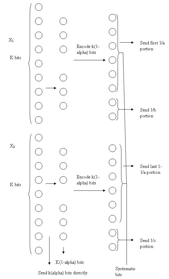
We have two sources and each of k bits. The scheme has been shown in Figure 8. Send a portion k*alpha of the bits equally spaced directly to the receiver. From the remaining k(1-alpha) bits, encode them using (( -alpha)/(1-alpha), ( -alpha)/(1-alpha) , , )-SW Distributed code defined earlier where , , and are respectively the desired source rates for the two sources and the forward and backward capacities of the channel between the two sources.
Decoding:
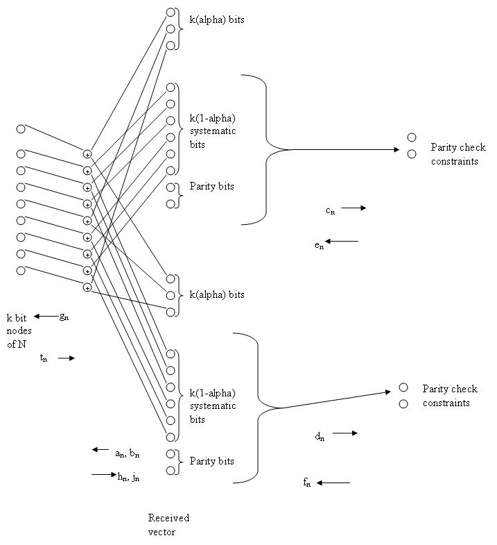
The decoding approach has been shown in Figure 9. The steps of message parsings in the scheme are:
- 1.
Message Parsing from the bit nodes to the Markov Model: The systematic bits of the two sources and the k*alpha bits that were sent without any encoding are used to get the likelihoods of the bits of N, as N is the sum of the two sources, and hence we can easily get their likelihoods from the likelihoods of the bits of the two sources. The likelihoods of the nodes of the received vector corresponding to the systematic bits of the two sources be and respectively with n denoting the bit with n varying from 1 to k and the ordering is according to the ordering in the input source vector of the two sources, then the likelihoods of the nodes of N are given by
- 2.
Message Parsing from Markov Model to the bit nodes: After receiving the noisy version of N, and knowing the memory structure of N, we can use trellis decoding to update the likelihoods of N and send the likelihoods towards the bit nodes. Consider the trellis for a finite-state binary Markov model. The starting and ending states associated with a particular edge are represented by and , respectively, and the bit corresponding to is denoted by . The trellis has two parallel branches between states (one associated with the bit and the other with the bit ). Each one of the branches in the trellis will have an associated a priori probability , which is obtained from the parameters of the Markov Model. The resulting equations that implement the belief propagation algorithm over the Markov model are given by
where is the normalizing factor so that . Now, this message foes back to the systematic portion of the bit nodes. Using we update the less reliable of the systematic bit nodes of the two sources by the xor operation. The systematic bits of two sources are updated by messages and respectively. Let us consider message update of , will be similar. The update equations for are given by
Since one of or will be known perfectly (by the encoding scheme), this just means to update the other if that is not known perfectly.
- 3.
Message Parsing from the bit nodes to the check nodes: This message propagation is from the k(1-alpha) systematic bits and the parity bits to the check nodes using their respective likelihoods, likelihoods of the systematic nodes given by and and those of parity bits the same as the initial likelihoods in the first iteration and those updated from the previous iteration from check nodes to bit nodes later. This message parsing is the same as the standard belief propagation scheme
- 4.
Message Parsing from the check nodes to the bit nodes: Using the belief propagation, we send the updated likelihoods towards the bit nodes.
Hence, the overall scheme can be summarized as:
- 1.
Message parsing from bit nodes to Markov model and back to the bit nodes.
- 2.
Message parsing from bit nodes to check nodes.
- 3.
If the parity equations are not satisfied, and iterations are less then maximum-iterations(say 100) go to Step 1 after message parsing from the check nodes to the bit nodes.

V Simulations of Distributed Source coding for Markov correlation
Take the source correlation model as a Markov source with two states with probability of 0 as one, and with probability of 0 as zero, and the transition probability from to and from and are the same and equal to p, the parameter which decides the entropy rate in the plot. Also, take the first source to be i.i.d, making = = 1-h(p). Take k=6250, alpha=.2, and = = 0.75. Hence, we send 6250*.2=1250 bits of each source without encoding and for the remaining bits we use the equations (3) and (4) with = .6875, and = = .5, we get a=2, b=1, c=1, R=.8421. The simulation with varying value of p is shown in Figure 10.
VI Conclusions
This work deals with the duality between source and channel coding. We take ideas developed for channel coding and transform them appropriately to construct joint source channel coding techniques. Distributed source coding scheme is a special case of the above work with the capacity of the channels to be equal to 1. We illustrated how to do joint distributed source channel coding at arbitrary source rates in the Slepian-Wolf rate region with arbitrary memoryless source correlation and arbitrary channel. We also illustrated how to do distributed source coding at arbitrary point in the Slepian-Wolf rate region when the source correlation model has memory. In all the simulations, we considered regular (3,x) LDPC codes. Taking irregular codes instead may perform better due to irregularity in the coding scheme.
Further work can be done to extend the distributed source coding for sources with Markov correlation to joint source channel coding. Joint source channel coding for sources with memory has been studied in [27][28]. Some work on the asymmetric case for this problem has also been done using turbo codes in [29]. But the problem using LDPC codes and doing for general source rates are still open problems.
References
- [1] D. Slepian and J. K. Wolf, Noiseless coding of correlated information sources, IEEE trans on Information theory, vol. 19, pp. 471 - 480, July 1973.
- [2] S. S. Pradhan and K. Ramchandran, Distributed source coding using syndromes (DISCUS): design and construction, Proc. IEEE Data Compression Conference, pp. 158-167, March 1999.
- [3] J. Li and R. Hu, Slepian-Wolf Cooperation: A Practical and Efficient Compress-and-Forward Relay Scheme Proceeding of 43rd Annual Allerton Conference on Communication, Control and Computing (Allerton) , St. Louis, MO, Nov. 2005.
- [4] D. Schonberg, K. Ramachandran, S.S. Pradhan, Distributed code constructions for the entire Slepian-Wolf rate region for arbitrarily correlated sources Proceedings of the Data Compression Conference, 2004.
- [5] S. S. Pradhan and K. Ramchandran, Distributed source coding: symmetric rates and applications to sensor networks, Proc. IEEE Data Compression Conference, pp. 363-372, March 2000.
- [6] J. Garcia-Frias, Joint source-channel decoding of correlated sources over noisy channels, Proc. IEEE Data Compression Conference, pp. 283-292, 2001.
- [7] A. Aaron and B. Girod, Compression with side information using turbo codes, Proc. IEEE Data Compression Conference, pp. 252-261, April 2002.
- [8] P. Mitran and J. Bajcy, Turbo source coding: A noise-robust approach to data compression, Proc. IEEE Data Compression Conference, p. 465, April 2002.
- [9] A. D. Liveris, Z. Xiong, and C. N. Georghiades, A distributed source coding technique for correlated image using turbo codes, IEEE Comm. Letters, vol. 6, pp. 379-381, Sept. 2002.
- [10] J. Garcia-Frias and Y. Zhao, Compression of correlated binary sources using turbo codes, IEEE Comm. Letters, vol. 5, pp. 417-419, Oct. 2002.
- [11] D. Schonberg, K. Ramchandran, and S. S. Pradhan, LDPC codes can approach the Slepian-Wolf bound for general binary sources, Proc. of fortieth Annual Allerton Conference, Urbana-Champaign, IL, Oct. 2002.
- [12] A. D. Liveris, Z. Xiong, and C. N. Georghiades, Compression of binary sources with side information at the decoder using LDPC codes, IEEE Comm. Letters, vol. 6, pp. 440-442, Oct. 2002.
- [13] Mina Sartipi and Faramarz Fekri, Distributed source coding in wireless sensor networks using LDPC coding: The entire Slepian-Wolf Rate Region IEEE Communications Society WCNC 2005.
- [14] H. Pishro-Nik and F. Fekri, Results on punctured low-density parity check codes and improved iterative decoding techniques Submitted to IEEE Transactions on Information Theory.
- [15] M. Mitzenmacher,A note on low density parity check codes for erasures and errors, SRC Technical Note 1998-017, December 1998.
- [16] J.G. Frias and W. Zhong, LDPC codes for compression of multi-terminal sources with hidden Markov correlation, IEEE Communication Letters, Vol. 7, No. 3, Mar 2003.
- [17] J.G. Frias,Decoding of low-density parity-check codes over finite-state binary Markov channels, IEEE Transactions on Communications, Vol. 52, No. 11, Nov. 2004.
- [18] Giuseppe Caire, Shlomo Shamai, and Sergio Verdu,Noiseless data compression with low-density parity-check codes, Advances in Network Information Theory P. Gupta, G. Kramer and A. J. van Wijngaarden, Eds., DIMACS Series in Discrete Mathematics and Theoretical Computer Science, vol. 66, pp. 263-284, American Mathematical Society, 2004
- [19] A. D. Liveris, Z. Xiong and C. N. Georghiades ,Joint source-channel coding of binary sources with side information at the decoder using IRA codes, Multimedia Signal Processing, 2002 IEEE Workshop on 9-11 Dec. 2002 Page(s):53 - 56
- [20] R. Hu, R. Viswanathan and Jing Li ,A new coding scheme for the noisy-channel Slepian-Wolf problem: separate design and joint decoding, GLOBECOM ’04. IEEE Volume 1, 29 Nov.-3 Dec. 2004 Page(s):51 - 55 Vol.1
- [21] J. Garcia-Frias and Y. Zhao , Near-Shannon/Slepian-Wolf performance for unknown correlated sources over AWGN channels, IEEE Transactions on Communications, Volume 53, Issue 4, April 2005 Page(s):555 - 559
- [22] W. Zhong and J. Garcia-Frias,LDGM Codes for Channel Coding and Joint Source-Channel Coding of Correlated Sources, EURASIP Journal on Applied Signal Processing 2005:6, 942-953
- [23] R. G. Gallager, Low-density parity-check codes, MIT Press, 1963.
- [24] T. J. Richardson and R. L. Urbanke, The capacity of low-density parity-check codes under message-passing decoding, IEEE Trans. Information Theory 47 (Feb. 2001), 599-618.
- [25] A. Wyner, Recent results in the Shannon theory, IEEE Trans. Inform. Theory, vol. 20, pp. 2 - 10, January 1974.
- [26] C. Berrou and A. Glavieux, Near optimum error correcting coding and decoding: turbo-codes, IEEE Trans. Communications, vol. 44, pp. 1261-1271, October 1996.
- [27] G. Caire, S. Shamai and S. Verdu, Almost-noiseless joint source-channel coding-decoding of sources with memory, 5th International ITG Conference on Source and Channel Coding (SCC), Jan 14-16, 2004
- [28] J. Garcia-Frias and J. D. Villasenor,Joint turbo decoding and estimation of hidden Markov sources, IEEE Journal on Selected areas in Communications, Vol. 19, No. 9, Sept. 2001
- [29] J. D. Ser, P. M. Crespo and O. Galdos, Asymmetric joint source-channel coding for correlated sources with blind HMM estimation at the receiver, EURASIP Journal on Wireless Communications and Networking 2005:4, 483-492