Enforced neutrality and color-flavor unlocking
in the three-flavor Polyakov-loop NJL model
Abstract
We study how the charge neutrality affects the phase structure of three-flavor PNJL model. We point out that, within the conventional PNJL model at finite density the color neutrality is missing because the Wilson line serves as an external “colored” field coupled to dynamical quarks. In this paper we heuristically assume that the model may still be applicable. To get color neutrality one has then to allow non vanishing color chemical potentials. We study how the quark matter phase diagram in -plane is affected by imposing neutrality and by including the Polyakov loop dynamics. Although these two effects are correlated in a nonlinear way, the impact of the Polyakov loop turns out to be significant in the direction, while imposing neutrality brings a remarkable effect in the direction. In particular, we find a novel unlocking transition, when the temperature is increased, even in the chiral limit. We clarify how and why this is possible once the dynamics of the colored Polyakov loop is taken into account. Also we succeed in giving an analytic expression for for the transition from two-flavor pairing (2SC) to unpaired quark matter in the presence of the Polyakov loop.
pacs
12.38.Aw,12.38.MhI Introduction
Quantum chromodynamics (QCD) is expected to exhibit a variety of phases depending on the temperature and on the baryon density [1]. At zero density and finite temperature the two main features of QCD are the confinement/deconfinement phase transition and chiral symmetry restoration. They should be realized when the hadronic system is heated, for example in ultrarelativistic heavy ion scattering processes such as at the Relativistic Heavy Ion Collision (RHIC) experiment [2] or in the future ALICE experiment at the Large Hadron Collider (LHC) at CERN. Moreover this behavior is clearly seen by lattice QCD simulations [3]. In these conditions quarks and gluons should be released as active degrees of freedom at some critical temperature. Moreover in the same range of temperatures one expects the restoration of chiral symmetry, whose spontaneous breakdown is known to play a key role in the mass spectroscopy of zero density QCD [4, 5]. At finite baryon densities similar transitions are also expected although the comparison with lattice simulation data is still lacking due to the so called fermion sign problem. However, at extremely high density, where perturbative techniques are allowed, it is now theoretically well established that quarks are deconfined forming diquark condensates so that the system is in a color superconducting ground state with asymptotic color-flavor locking (CFL) [6]. While difficult to achieve in the laboratory color superconductivity might be relevant to the inner structure of compact stellar objects [7].
Exploring phase structure at intermediate density, where neither lattice simulations nor perturbative calculations can be trusted, is the object of various model studies. There are different effective models which provide simple descriptions of chiral symmetry restoration at finite temperature and density; the Nambu-Jona Lasinio (NJL) model is one of them [4, 5, 8, 9]. The NJL model realizes the spontaneous chiral symmetry breaking of QCD at small temperature and density. Despite its simple structure, it can also realize a CFL phase at the largest density. Moreover it can even reproduce the correct ratio of the gap and critical temperature for the transition from the CFL to the unpaired phase.
The main defect of the NJL model is the absence of the confinement/deconfinement transition. A theoretical attempt to understand the nature of the deconfinement transition goes back to the work [10] in which deconfinement was shown to be associated with the spontaneous breaking of the global -symmetry of a finite temperature pure gauge theory. The order parameter is the traced Polyakov loop, whose condensation and correlation are related to the free energy of static quark and the string tension between two static quarks in a thermal medium.
The inclusion of the Polyakov loop dynamics into the NJL model was first done by Fukushima [11] in order to study the relation between chiral restoration and deconfinement. It is now called “Polyakov loop extended Nambu-Jona Lasinio” (PNJL) model. In this model, the chiral condensate serves as an order parameter for the chiral transition, while the traced Polyakov loop performs this job for the deconfinement transition. Even though the former and the latter have their definite meanings, as order parameters, only within different limits, ( and ), they are still useful as indicators of both crossovers and/or transitions. In addition, the model enables to interpret nicely some bulk properties of matter observed on the lattice on the field theoretical ground [12].
The purpose of this work is to investigate the color superconducting phase structure in -plane within the PNJL model, and to study the effect of imposing neutralities, in both the paired and unpaired phases, in presence of the Polyakov loop. The neutrality constraints are known to be important for the candidates of color superconducting phases at a realistic density; they open a window in a phase diagram to intriguing gapless phases [13, 14]. Although a few works have already explored the pairing phases of PNJL models [15, 16, 17], none of them takes into account either the possibility of complicated gap structures or the neutrality effects. Thus our study is a natural extension of them. One surprising result is that once PNJL model is applied to finite density, it inevitably lacks color neutrality even when the system is unpaired. This is a sort of sign problem at finite density. In this paper we still proceed on the heuristic assumption that PNJL is applicable to finite densities. Also it will turn out that the inclusion of the Polyakov loop greatly affects the phase diagram by stabilizing the two-flavor pairing (2SC) phase, and it also brings about a color-flavor unlocking transition [18] at finite temperature in a new mechanism.
The paper is organized as follows. In Sec. II, we introduce our model and approximations. In the first part of Sec. III, we demonstrate the lack of color neutrality in the conventional PNJL model at finite density. The rest of the section is devoted to discussion of the numerical results. The neutrality effects, the effect of dynamics of Polyakov loop, and their interplay will be particularly covered. We summarize the main contents of our paper with some concluding remarks in Sec. IV.
II Formalism
In order to accommodate for pairing in the channel at finite density, we add the 4-point vertex to the free part of the Polyakov-quark model, which hereafter we shall refer to as the Polyakov NJL (PNJL) model.
| (1) |
Here stands for the quark field, and a summation over color and flavor degrees of freedom is understood. () is the matrix, antisymmetric in color, flavor and spin, specifying the pairing channel. The constant parameterizes the strength of the coupling leading to diquark condensation. We work within the chiral limit, setting , and take into account the strange quark mass within the high density approximation. This means that we include the effect of its finite value in the chemical potential difference [13]. As a result,
| (2) |
where , , and , with being the standard Gell-Mann matrices. We find it more transparent switching to a new spinor basis for the quark field defined as by means of:
| (3) |
with unitary matrices in color and flavor space defined in [19]. In this new basis (2) takes the form of a diagonal matrix: with .
We treat the Polyakov loop by the static, homogeneous, and classical background gauge field where the temporal gauge field is introduced by parameterizing the Wilson-line, as . In the PNJL model one assumes that this background gauge field couples to quarks with covariant derivative . In the convenient gauge called Polyakov gauge, the Wilson line is in the diagonal representation [11],11 1 One can always find the gauge rotation such that becomes diagonal. This is simply a gauge fixing, and any physical quantities will not depend on the gauge freedom so we can safely reduce the eight dynamical variables to parametrize up to two independent parameters . We note, however, when the diquark condensation is taken into account, this is no longer justified unless more general ansatz for the diquark condensation, , is adopted. Simultaneous color-flavor rotation can make the condensate matrix diagonal such that the usual assumption, ,is recovered, but this is nothing but the gauge fixing. Thus in principle, if we adopt the diagonal ansatz for the diquark condensation, we can no longer make gauge rotated to diagonal, and on the other hand, if we adopt the diagonal form of , we should work in more general assumption for . Nevertheless, we work in the simplified assumption that both and are of diagonal as in [15] leaving a further detailed analysis in the future. i.e.,
| (4) |
Moreover we restrict ourselves to the case such that the traced Polyakov loop becomes real [15] whereas at finite density there is no strict reason why should be real [20, 21]. Thus in this representation, , and the effect of the background field is just to shift the color chemical potential to the imaginary direction . For the Polyakov loop effective potential we use the following form, inspired by the strong coupling analysis of the pure gauge sector [22, 11, 23]
| (5) |
with
| (6) |
The numerical values for coefficients are determined by fitting several quantities to the lattice results of pure gauge theory [12]:
| (7) |
In the absence of dynamical quarks, is set to the value of the transition temperature for deconfinement, i.e., . In our model, we use the value which is the theoretically suggested value for in the presence of two light flavors, [12, 24], although as we treat the strange quark mass as a free parameter, our calculation will cover the situations between two flavor and three flavor, i.e., . In the case , the slightly lowered value is proposed, but we have checked that choosing this value for does not change our results in any significant way.
By introducing a charge conjugated field as an independent field, and after introducing the Hubbard-Stratonovich field and , we integrate out the fermion field . Within the mean field approximation for and , the effective potential becomes
| (8) |
where with denoting the imaginary time, and the transpose operation only acts on the color and flavor structure of .
It is useful to write down the thermodynamic potential in the and case. Leaving the trace over color, it takes a form
| (9) |
with . Within the Polyakov gauge and imposing the prescription, the Wilson line takes the following form
| (10) |
with .
Let us now consider the case with and . We try to simplify the expression for the thermodynamic potential. Within the current approximation (treating as a shift of the chemical potential), the action does not mix the left-handed quark and the right handed quarks. Thus, we can rewrite the functional determinant as
| (11) |
Now the Dirac gamma matrices can be regarded as two dimensional matrices for Weyl spinors, say, . Finally, putting with velocity , and discarding the antiquark contributions, we get the high density effective theory (HDET) approximation for the effective potential [25].
| (12) |
where is a momentum cutoff, and the positive energy left handed projected propagator is defined as
| (13) |
This is now a matrix defined in the color-flavor space. It has a form . In order to evaluate the Matsubara summation, we have to evaluate all the eigenvalues of the hamiltonian density . Since we have doubled the degrees of freedom by introducing the Nambu-Gorkov notation, the eigenvalues of the hamiltonian will appear as with . In contrast to the standard NJL models without Polyakov loop, is no longer Hermitian due to the imaginary chemical potential , and accordingly each quasiparticle energy can take in general complex values. Consequently, is no longer restricted to be real. We avoid this sign problem by taking the real part of as in [12]. Once these quasiparticle energies are evaluated, and choosing the basis as such that both the conditions, and when , are satisfied, we can perform the Matsubara summation as
| (14) |
We took the energy density in the vacuum without any condensation as the reference energy density. The fifth term is nothing but the zero temperature part of free quark contribution to the effective potential. We need the ultra violet cutoff only in the integral representing the condensation energy, i.e., the last term.22 2 The integral of the thermal part () can be evaluated without cutoff. Instead of , we use , the zero temperature CFL gap in the chiral limit without Polyakov loop, as the indicator of diquark attraction [26]
| (15) |
With the use of this cutoff dependent coupling constant, the derivatives of the effective potentials, , now have well-defined limits as . In this way, we can remove the cut-off dependence from the gap equations, while it remains in the effective potential itself.
The evaluation of the effective potential is carried out by finding the eigenvalues of for given momentum , and integrating them over the momentum. Then the mean field solution for the ground state is obtained by minimizing the effective potential with respect to imposing the proper constraints of charge neutrality, .
III Results
In this section, for the numerical computations we fix , and concentrate on the case with with . We would study the phase diagram, and how the physical quantities behave as functions of , and temperature , treated as free parameters. In the numerical calculations, in order to take the minimum strong coupling effect into account, we bring back the momentum dependence of the density of state . By doing this, the particle-hole asymmetry which is known as the first correction to the weak coupling approximation will be properly taken into account.
III.1 Color neutrality
Before discussing in detail the calculation let us briefly comment on a strange feature that shows up, even in the unpaired phase (), if one assumes vanishing charge chemical potentials. The interesting fact is that the conventional PNJL model calculation at finite lacks color neutrality. It is worth stressing here that this does not follow from HDET approximation (see (9) obtained before introducing HDET formalism). It is clear from (10) that the Wilson line couples to each color of quarks, , with different weight. Looking at the real part only, the weight for quarks differs from that of quarks. Thus, the energy required to populate quarks in the background gauge field is different from that for quarks. Furthermore, can take a negative value close to when the system is nearly confined. This means that thermal excitations of on-shell quarks reduce the pressure of the system making it difficult to create on-shell quarks in the system. This can be regarded as the effect of confinement in this PNJL model at finite density. The problem is that, even in this situation, quarks can be excited at finite temperature because is unity and thus the thermal weight for quarks does not differ from that in the deconfined phase. This unphysical feature might be viewed as an artifact of this PNJL model which originates in the assumption that the dynamics of traced Polyakov loop can be equivalently described by the constant background gauge field . As a consequence, the development of the finite value of breaks not only the center symmetry but also the color symmetry in a spontaneous way; this fact does not contradict the Elitzur’s theorem [27] since we still expect physical quantities such as quasi-particle dispersions should not depend on the gauge and thus have their definite meanings even after gauge unfixing which would make itself vanish.
One may think that this undesired feature is just due to the wrong ansatz of the PNJL model itself. Apart from such a possibility, in order to avoid an unphysical appearance of color density within the model, we should inevitably introduce an appropriate color chemical potential. According to the gauge of the Polyakov loop, in our case, is required to maintain the unpaired phase color neutral. To be more explicit, ignoring the antiquarks we can write the color density as
| (16) |
where is just the density of a free Fermi gas and
| (17) |
is the modified Fermi distribution in the presence of describing quarks which is plotted in Fig. 1(b) compared to the standard Fermi distribution for blue quarks. From (17) it follows that the density of and quarks differs from that of simple fermi gas, and the difference never disappears unless either or is approached. The difference also cancels at thanks to the equal and opposite contribution from antiquarks.

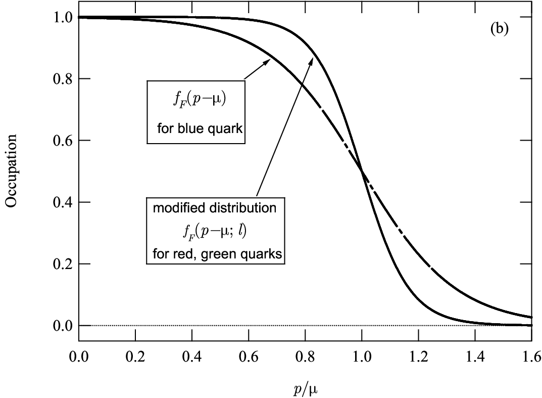
In Fig. 1(a), we plot the ratios of each color density, , , and , to the total quark density as a function of in the unpaired phase with . In the numerical evaluation we set , and ignore the tiny antiquark contributions. As discussed above, we can see the finite difference between and in the intermediate range of temperature.33 3 It should be noted that the color density itself is a gauge dependent quantity and thus should depend on the choice of the gauge parametrizing the Wilson line. With our diagonal representation of Eq. (4) with , the color density becomes finite as we observed above. If we selected the different gauge, the other entry of octet color densities should have appeared. The important thing is, however, whichever gauge we choose,some color density should become finite; in fact the squared sum of the octet color densities is shown to be the gauge independent quantity [28]. The deviation becomes maximum near the steepest point of the Polyakov loop, which is usually identified as the deconfinement transition [12].
III.2 Phase diagrams
In Fig. 2(a), the phase diagram in the -plane of the charge neutral PNJL model is displayed. The bold line represents the first order phase transition, while the thin line represents the second order phase transition. The dashed line corresponds to the crossover from the 2SC phase to the gapless 2SC (g2SC) phase. For comparison, we have shown in figure 2(b) the phase diagram for the charge neutral NJL model which is the same reported in [29]. We are specifying each phase as summarized in TABLE 1.
| (g)CFL | for with or satisfied |
|---|---|
| dSC | , |
| uSC | , |
| (g)2SC | , with satisfied |
From these graphs, the impact of the Polyakov loop dynamics on the pairing is quite obvious. The inclusion of the temporal gluon field significantly broadens the region for the superconducting phase, in particular for the 2SC phase. In fact, the critical temperature is almost twice as large as that in the NJL model without the Polyakov loop which is already known in [15]. (Note that the scale for the -axis of figure (a) is twice as that of figure (b).) Apart from this significant quantitative change, the qualitative behavior of the phase diagram is not so much affected. In both cases, the d-quark superconducting phase (; dSC) exists in a small region at finite temperature [30, 29], and there is the doubly critical point indicated by the upper triangle, a point where the line for the vanishing of intersects that for [29]. Also the existence and the location of the critical point where the fully gapped CFL phase turns into the gapless CFL (gCFL) phase phase is not affected. In both figures the point is indicated by a lower triangle on the axis. This fact means the the effect of the Polyakov loop on the pairing is absent at . The reason is that at the Polyakov dynamics decouples from the pairing (NJL) dynamics so that the effect is absent because the temporal gauge field is proportional to itself.


III.3 Impact of the Polyakov loop at finite temperature; color-flavor unlocking and stiff 2SC phase
Next we focus in detail on the phase transitions at in order to study the impact of the Polyakov loop dynamics and charge neutrality. To this end, we examine each effect step by step. In Fig. 3(a), we show the gaps (solid lines) and the Polyakov loop (long-dashed one) calculated without the neutrality. For comparison, we also show by the dashed line the calculated with the NJL model without the Polyakov loop. In this case, the three gaps have the same behavior as functions of and they drop to zero simultaneously when (shown by the bold square on the axis) is approached. Once the Polyakov loop is taken into account this is no longer true as one can see from the figure. Two gaps have the same magnitude, , while is larger; moreover the two gaps drop to zero simultaneously near a point lower than the bold square (). This can be described as a second order color-flavor unlocking transition induced by the Polyakov loop dynamics. This behavior is not strange because even though the Polyakov loop is blind to the flavor degrees of freedom, in the color-flavor locked phase, however, color is locked to flavor which is the way the Polyakov loop affects the gap structure. In fact, as we have already discussed in Sec. III.1, the presence of the Polyakov loop induces a finite color density as in the unpaired phase. This means that the existence of the Polyakov loop adds to the real part of the effective potential, , the finite external field with charge, which explicitly breaks global color down to . Since color and flavor are locked in the CFL phase, the external field induced by tends to break the symmetry down to . This is the very reason for the splitting, and also for the color-flavor unlocking to the 2SC phase. The emergence of color-flavor unlocking is one of the most interesting features of the inclusion of the Polyakov loop dynamics in NJL model.


A further aspect deserves to be stressed. The 2SC phase persists up to which is almost twice as large as the weak coupling formula for the critical temperature, (indicated by the bold square). This striking feature is already noticed in the limiting case with the pure CFL ansatz using the Ginzburg-Landau approach [16]. In what follows, we try to explain this fact. In the case of the 2SC case, we can explicitly determine the quasiparticle energy dispersion. Four out of nine quasiquarks have nontrivial dispersion laws: and . In this case, there is no shift of the averaged chemical potential to the imaginary direction. The gap equation in the absence of charge chemical potentials then becomes
| (18) |
where is the Fermi distribution, and its energy argument is now supposed to be . The second term proportional to is referred to as a blocking integral due to thermally excited quarks. We need no cutoff for this part to be evaluated. We notice that the effect of the temporal gauge field is just to suppress the blocking integral. This explains the robustness of 2SC in the presence of , and the increase of the critical temperature as follows. We put in (18) and try to solve it in to derive the critical temperature. (18) with is nothing but the condition for criticality, the Thouless criterion, which guarantees the divergent susceptibility. This condition together with the definition of the effective coupling coupling constant (15) leads to
| (19) |
Note that the quantity is dimensionless and does not depend on . In the case of the deconfinement phase with , vanishes so that it simply reproduces the standard expression for the critical temperature . It is now easy to imagine that the deviation of from unity leads to the positive , and thus increases the critical temperature . To the first order in , can be calculated as
| (20) |
Thus to this order, the critical temperature is approximated by
| (21) |
near . When is substituted into the above formula, gets the factor of enhancement . Although it is within the linear level, this value fairly agrees with the numerically obtained factor, . If we use the numerical value of , the factor of enhancement becomes ; the agreement is perfect. Although unrealistic, at (the confinement), the analytical evaluation is also possible. In this case we have so that we have the factor . This is the theoretical maximum of the critical temperature in the PNJL model at weak coupling.
III.4 Effect of charge neutrality; the two-step hierarchical unlocking transition
Let us now discuss charge neutrality at . In Fig. 3(b), we show the gaps and chemical potentials as a function of calculated respecting the charge neutrality constraints. For comparison, we have shown without neutrality (in Fig. 3(a)) by a dashed line. At a first glance, we notice that, even quantitatively, the charge neutrality plays only a minor role at .
However, several interesting remarks deserve a discussion here. (i) First, the charge neutrality conditions lift the degeneracy away and open a small window for the dSC phase between the CFL and 2SC phases. (ii) Second, vanishes when the 2SC phase sets in. (iii) Lastly, does not vanish even when all the pairing melt and the system goes into the unpaired quark matter as already discussed in Sec. III.1 in the case of no pairing at all. Without finite , the unpaired system inevitably has a finite -color charge. The reason for (ii) is simple. The 2SC pairing preserves the symmetry intact or, in other words, the 2SC gap has singlet structure and is transparent to the charge. Therefore the system with no -color charge should have . One may think that a finite value of induces a finite charge in the system with , but this is not correct. In fact, as we saw in the discussion in Sec. III.1, restricting ourselves to the real part of , is realized in the unpaired system inducing a charge but no charge. The point (i) can be understood as follows. In the presence of , the gaps split as as we saw above. This induces an imbalance in the thermal population of nine quasiquarks in the CFL phase. Accordingly, the charge neutrality is lost unless , and are tuned to their appropriate values. But of course the finite values of and explicitly break the remaining symmetry. As a result of this secondary effect, the degeneracy should be lifted away, as . The appearance of the dSC phase at is in contrast either to the Ginzburg-Landau approach [30] or to the pure NJL calculations [29]; this is definitely due to the nontrivial interplay between the neutrality constraints and the Polyakov loop dynamics.
III.5 Effect of the stress due to nonzero strange quark mass
Let us now discuss the effect of a nonzero strange quark mass on the structure of gaps. In Fig. 4(a) we show the zero temperature gaps as functions of , both for the CFL (solid lines) and 2SC (dashed line) solutions. The free energy comparison shows that there is a first order phase transition from the gCFL phase to the g2SC phase at the point indicated by the vertical dash-dotted line in the figure. Since at the Polyakov loop dynamics decouples from the pairing (NJL) sector, the Polyakov loop plays no role in the gap structure. Consequently, the phase structure and the behavior of the gaps is similar to the result of [29] although the HDET approximation was not adopted there.
At low , the CFL phase is realized, and it continuously goes into the gCFL phase [13] at a point slightly lower than . Then eventually the gCFL phase is taken over by the g2SC phase at by a first order transition [14, 29].


In Fig. 4(b), we have shown the gaps at a finite temperature, . The first order transition is completely washed away, and there are two successive second order unlocking transition until the system gets unpaired, first from the CFL phase to the uSC phase, and subsequently from the uSC phase to the 2SC phase. This feature is also qualitatively the same as in the NJL calculations [29].
III.6 Interplay of the Polyakov loop dynamics and enforced neutrality at finite strange quark mass
Let us finally examine the impact of enforcing charge neutralities and including the Polyakov loop dynamics into the pairing phases at an intermediate density represented by the finite value of . In Fig. 5(a) the gap and the charge chemical potentials are depicted as functions of at . At this value of the stress, the CFL pairing is not possible, so only the (g)2SC phase can show up as a pairing pattern. What is surprising and also intriguing is that once melts at but appears again at higher temperature about , and then finally vanishes completely when exceeds . The 2SC phase exists in two different region in temperature. This feature is definitely due to the inclusion of both the neutrality and the Polyakov loop into the problem. To see this, we show in Fig. 5(b), the gaps calculated with simplified versions of our PNJL model. The solid line indicated by “Full” is the same as in Fig. 5(a). The long-dashed line represents the result calculated using the pure NJL model without the Polyakov loop dynamics, while the dashed line is that calculated with PNJL model but without imposing the charge neutrality constraints, i.e., putting from the very beginning.


From these comparisons, it is clear that the appearance of the intriguing possibility of the existence of two islands of 2SC in temperature is due to the combinatory, cooperative effect between the Polyakov loop dynamics and the neutrality constraints. In contrast to the case with , imposing neutrality has a sizable effect on the gap. It significantly reduces the magnitude of the gap. It is so because in the case of a finite value of , not only but also should be finite even in the unpaired phase in order to guarantee electrical neutrality. Moreover the effect of the Polyakov loop is not only to stabilize the 2SC phase against the increase of temperature as in case, but also to suppress the pairing at low temperature making two separated islands of 2SC in temperature.
IV Summary
In this paper, we have studied the quark matter phase structure in plane starting from the PNJL model in which a temporal static gluon field couples with quarks. This work is a natural extension of previous studies [15, 16, 17]. The particular focus was put on the effects produced by the inclusion of the Polyakov loop dynamics on the pairing phases and by the enforcement of color and electrical neutrality.
In the conventional PNJL model, there is a mismatch in each color density so that the model lacks the color neutrality even in the unpaired phase. This unphysical feature is significant in the proximity of the deconfinement transition. We have pointed out that this behavior may be due to the original assumption hidden in the PNJL model i.e.that the traced Polyakov loop dynamics can be represented by the inclusion of the static temporal “colored” gauge field which couples to the fundamental color charge of dynamical quarks. By this assumption one misses gauge invariance. Once this fact is admitted, in order to avoid the unphysical appearance of color densities within this model, one has to include the charge chemical potentials into the problem from the beginning. In fact, we have shown that should be finite to maintain color neutrality in the unpaired phase.
In the detailed numerical analysis, we have depicted the phase diagram in -plane, and clarified how the phase diagram is affected by the inclusion of the Polyakov loop and the enforcement of charge neutrality. Even at , the effect of the Polyakov loop is remarkable; it breaks the down to and causes a continuous color-flavor unlocking at finite temperature in a novel mechanism. In addition, it makes the 2SC phase much more robust against the increase of temperature. The critical temperature is about twice as large as the weak coupling prediction, which is consistent with previous calculations [15, 16, 17]. We have also examined a formal explanation about these facts and derived an analytical expression of this enhancement factor; it turned out that the temporal gauge field reduces a blocking integral.
The effect of imposing neutralities gives only a tiny effect at although it opens a small window for the dSC realization between the 2SC and CFL phases by lifting away the degeneracy. In this case, we have a hierarchical unlocking, CFL dSC 2SC, until it eventually goes into the unpaired phase. This is contrast to the pure NJL calculation without the Polyakov loop where the dSC never shows up at [29].
The sizable effect of imposing charge neutrality on the pairing phases manifests itself at finite . We have shown that the nontrivial, complicated interplay between the charge neutrality constraints and the Polyakov loop dynamics at produces a thermal reentrance phenomenon, as two isolated windows for the 2SC pairing can show up on the temperature axis.
There are several ways to extend our current study. One is to take the chiral condensation into account by including the chiral condensate and removing the high density approximation [31]. By this improvement, one can study the interplay between the chiral condensate, the Polyakov loop, and color superconductivity at the same time. The other possibility is to study mesonic modes [32, 33] as well as the Meissner masses in the superconducting phases. This might have an impact either on a possible meson condensation in superconducting phases or on the so called chromomagnetic instability problem in gapless phases [19, 34]. These studies may be presented elsewhere in future.
To conclude let us stress that two alternatives have presented to us:
a) application of the PNJL model to finite density is pathological and should be avoided, in relation to the fact that color neutrality is not visibly satisfied;
b) the model can be used also at finite density provided neutrality is enforced: for such a case we have derived the detailed consequences obtaining surprising results but without apparent physical inconsistencies.
We hope that further work will illuminate on the choice between a) and b).
We thank Kenji Fukushima, Mei Huang, Andreas Schmitt and in particular, Igor Shovkovy for enlightening discussion. One of us (H. A.) thanks I.N.F.N. for financial support. Numerical calculations were carried out on Altix3700 at YITP in Kyoto University, and on the workstation NETCLUS at University of Bari (I.N.F.N., Sezione di Bari).
References
- [1] K. Rajagopal and F. Wilczek, arXiv:hep-ph/0011333; D. H. Rischke, Prog. Part. Nucl. Phys. 52, 197 (2004) [arXiv:nucl-th/0305030].
- [2] I. Arsene et al. [BRAHMS Collaboration], Nucl. Phys. A 757, 1 (2005); B.B. Back et al. [PHOBOS Collaboration], Nucl. Phys. A 757, 28 (2005); J. Adams et al. [STAR Collaboration], Nucl. Phys. A 757, 102 (2005); K. Adcox et al. [PHENIX Collaboration], Nucl. Phys. A 757, 184 (2005).
- [3] C. Bernard et al. [MILC Collaboration], Phys. Rev. D 71, 034504 (2005); M. Cheng et al. [RBC-Bielefeld Collaboration], Phys. Rev. D 74, 054507 (2006); Y. Aoki, Z. Fodor, S. D. Katz and K. K. Szabo, Phys. Lett. B 643, 46 (2006).
- [4] Y. Nambu and G. Jona-Lasinio, Phys. Rev. 122, 345 (1961).
- [5] T. Hatsuda and T. Kunihiro, Phys. Rept. 247, 221 (1994) [arXiv:hep-ph/9401310]; S. P. Klevansky, Rev. Mod. Phys. 64 (1992) 649.
- [6] M. G. Alford, K. Rajagopal and F. Wilczek, Nucl. Phys. B 537, 443 (1999) [arXiv:hep-ph/9804403];
- [7] For a review, see, F. Weber, Prog. Part. Nucl. Phys. 54, 193 (2005) [arXiv:astro-ph/0407155].
- [8] M. Asakawa and K. Yazaki, Nucl. Phys. A 504, 668 (1989).
- [9] R. Rapp, T. Schafer, E. V. Shuryak and M. Velkovsky, Phys. Rev. Lett. 81, 53 (1998) [arXiv:hep-ph/9711396]; M. G. Alford, K. Rajagopal and F. Wilczek, Phys. Lett. B 422, 247 (1998) [arXiv:hep-ph/9711395].
- [10] A. M. Polyakov, Phys. Lett. B 72, 477 (1978); L. Susskind, Phys. Rev. D 20, 2610 (1979); B. Svetitsky and L. G. Yaffe, Nucl. Phys. B 210, 423 (1982); B. Svetitsky, Phys. Rept. 132, 1 (1986).
- [11] K. Fukushima, Phys. Lett. B 591, 277 (2004) [arXiv:hep-ph/0310121].
- [12] C. Ratti, M. A. Thaler and W. Weise, Phys. Rev. D 73, 014019 (2006) [arXiv:hep-ph/0506234].
- [13] M. Alford, C. Kouvaris and K. Rajagopal, Phys. Rev. Lett. 92, 222001 (2004) [arXiv:hep-ph/0311286]; M. Alford, C. Kouvaris and K. Rajagopal, Phys. Rev. D 71, 054009 (2005) [arXiv:hep-ph/0406137].
- [14] I. Shovkovy and M. Huang, Phys. Lett. B 564, 205 (2003) [arXiv:hep-ph/0302142]; M. Huang and I. Shovkovy, Nucl. Phys. A 729, 835 (2003) [arXiv:hep-ph/0307273].
- [15] S. Roessner, C. Ratti and W. Weise, Phys. Rev. D 75, 034007 (2007) [arXiv:hep-ph/0609281].
- [16] M. Ciminale, G. Nardulli, M. Ruggieri and R. Gatto, Phys. Lett. B 657, 64 (2007) [arXiv:0706.4215 [hep-ph]].
- [17] M. Ciminale, R. Gatto, N. D. Ippolito, G. Nardulli and M. Ruggieri, Phys. Rev. D 77, 054023 (2008) [arXiv:0711.3397 [hep-ph]].
- [18] M. G. Alford, J. Berges and K. Rajagopal, Nucl. Phys. B 558, 219 (1999) [arXiv:hep-ph/9903502]; T. Schafer and F. Wilczek, Phys. Rev. D 60, 074014 (1999) [arXiv:hep-ph/9903503].
- [19] R. Casalbuoni, R. Gatto, M. Mannarelli, G. Nardulli and M. Ruggieri, Phys. Lett. B 605, 362 (2005) [Erratum-ibid. B 615, 297 (2005)] [arXiv:hep-ph/0410401].
- [20] A. Dumitru, R. D. Pisarski and D. Zschiesche, Phys. Rev. D 72, 065008 (2005) [arXiv:hep-ph/0505256].
- [21] K. Fukushima and Y. Hidaka, Phys. Rev. D 75, 036002 (2007) [arXiv:hep-ph/0610323].
- [22] J. Polonyi and K. Szlachanyi, Phys. Lett. B 110, 395 (1982); M. Gross, Phys. Lett. B 132, 125 (1983).
- [23] S. K. Ghosh, T. K. Mukherjee, M. G. Mustafa and R. Ray, arXiv:0710.2790 [hep-ph].
- [24] B. J. Schaefer, J. M. Pawlowski and J. Wambach, Phys. Rev. D 76, 074023 (2007) [arXiv:0704.3234 [hep-ph]].
- [25] For a review, see, G. Nardulli, Riv. Nuovo Cim. 25N3, 1 (2002) [arXiv:hep-ph/0202037].
- [26] T. Schafer, Nucl. Phys. B 575, 269 (2000) [arXiv:hep-ph/9909574].
- [27] S. Elitzur, Phys. Rev. D 12,3978 (1975).
- [28] M. Buballa and I. A. Shovkovy, Phys. Rev. D 72, 097501 (2005) [arXiv:hep-ph/0508197].
- [29] K. Fukushima, C. Kouvaris and K. Rajagopal, Phys. Rev. D 71, 034002 (2005) [arXiv:hep-ph/0408322]; H. Abuki and T. Kunihiro, Nucl. Phys. A 768, 118 (2006) [arXiv:hep-ph/0509172].
- [30] K. Iida, T. Matsuura, M. Tachibana and T. Hatsuda, Phys. Rev. Lett. 93, 132001 (2004) [arXiv:hep-ph/0312363].
- [31] H. Abuki, M. Kitazawa and T. Kunihiro, Phys. Lett. B 615, 102 (2005) [arXiv:hep-ph/0412382]; S. B. Ruester, V. Werth, M. Buballa, I. A. Shovkovy and D. H. Rischke, Phys. Rev. D 72, 034004 (2005) [arXiv:hep-ph/0503184]; D. Blaschke, S. Fredriksson, H. Grigorian, A. M. Oztas and F. Sandin, Phys. Rev. D 72, 065020 (2005) [arXiv:hep-ph/0503194].
- [32] H. Hansen, W. M. Alberico, A. Beraudo, A. Molinari, M. Nardi and C. Ratti, Phys. Rev. D 75, 065004 (2007) [arXiv:hep-ph/0609116].
- [33] H. Abuki, M. Ciminale, R. Gatto, N. D. Ippolito, G. Nardulli and M. Ruggieri, arXiv:0801.4254 [hep-ph].
- [34] M. Huang and I. A. Shovkovy, Phys. Rev. D 70, 051501 (2004) [arXiv:hep-ph/0407049].