The Fibonacci quantum walk and its classical trace map
Abstract
We study the quantum walk in momentum space using a coin arranged in quasi-periodic sequences following a Fibonacci prescription. We build for this system a classical map based on the trace of the evolution operator. The sub-ballistic behavior of this quantum walk is connected with the power-law decay of the time correlations of the trace map.
pacs
03.67.-a, 05.40.FbI Introduction
The quantum walk (QW) on the line is a subject that has drawn much attention in quantum computing [1]. It has been introduced by [2, 3], as counterpart of the classical random walk. Due to the success of the classical random walks in the description of many classic models of the nature, the possibility that future quantum algorithms will be based on the QW has attracted the attention of researchers from different fields. Additionally, as a result of recent advances in experimental techniques to manipulate quantum states has led the scientific community to think that quantum computers could be a reality in the near future. Anyway the study of the QW subjected to different sources of decoherence is a topic that allows to analyze and verify the principles of quantum theory and has been considered by several authors [4].
One of the most striking properties of the QW is its ability to spread over the line linearly in time as characterized by the standard deviation , while its classical analog spreads out as the square root of time []. Recently, in ref. [5] the QW was generalized introducing two coin operators arranged in quasi-periodic sequences following a Fibonacci prescription. This “Fibonacci QW” leads to an unexpected sub-ballistic wave function spreading, as shown by the power-law tail of the standard deviation [ with ]. More recently[6, 7], we have studied the QW subjected to noise with a Lévy waiting-time distribution [8], finding that the system has also a sub-ballistic wave function spreading instead of the known ballistic growth. The Fibonacci sequence gives rise to a rich behavior also in other systems; it is the cause of sub-ballistic behavior both for the quantum kicked rotor in resonance [9] and for tight-binding electrons [10, 11]. On the other hand Sutherland [12], twenty years ago, studied a very simple two dimensional system of a single particle with spin subjected to quasi-periodic external field pulses, showing that the dynamics of the system is determined by a three dimensional “trace map”. In that work, he found three regions of the parameters space characterized by qualitative differences of the decay of the time-correlation function: slower than a power law, as a power law, and faster than a power law.
Here we study the Fibonacci QW through the dynamics of its trace map. We show that the sub-ballistic behavior of the QW is connected with the power- law decay of the time-correlation function of the trace map.
II Fibonacci quantum walk
The dynamics of the Fibonacci QW will be generated by a large sequence of two time-step unitary operators and for each time . Given the two initial values of the succession and the sequence is obtained, as was done in previous works [13, 12, 5], using the rule
| (1) |
To obtain the operators and we develop in some detail the free QW model. The standard QW corresponds to a one-dimensional evolution of a quantum system (the walker) in a direction which depends on an additional degree of freedom, the chirality, with two possible states: “left” or “right” . Let us consider that the walker can move freely over a series of interconnected sites labeled by an index . In the classical random walk, a coin flip randomly selects the direction of the motion; in the QW the direction of the motion is selected by the chirality. At each time step a rotation (or, more generally, a unitary transformation) of the chirality takes place and the walker moves according to its final chirality state. The global Hilbert space of the system is the tensor product where is the Hilbert space associated to the motion on the line and is the chirality Hilbert space.
We shall consider only unitary transformations which can be expressed in terms of a single real angular parameter [14, 15, 16]. Let us call () the operators that move the walker one site to the left (right) on the line in and let and be the chirality projector operators in . Then we consider free evolution transformations of the form [14],
| (2) |
where is an unitary operator acting on , and being the standard Pauli matrices, and is the identity operator in . The unitary operator evolves the state by one time step,
| (3) |
The wave vector is expressed as the spinor
| (4) |
where we have associated the upper (lower) component to the left (right) chirality, the states are eigenstates of the position operator corresponding to the site on the line. The unitary evolution for , corresponding to Eq. (3) can then be written as the map
| (5) | ||||
To build the operators and we substitute in the previous expression by and respectively. As mentioned in the introduction these types of maps produce a sub-ballistic wave function spreading.
III Trace map
With the operators defined in the previous section, we shall study the Fibonacci QW connecting it explicitly with the work of Sutherland [12]. To this end, we make the spatial Fourier transform of the amplitude multiplying both sides of Eq. (5) by , with , and summing in the integer index :
| (6) |
where
| (7) | ||||
| (8) |
and
| (9) |
Thus in Fourier space, the dynamics of the Fibonacci QW is determined by the unitary matrix . We call and the matrix evaluated in and respectively. The matrix can be rewritten employing the Bloch-sphere representation as
| (10) |
where is the identity matrix, is given by
| (11) |
and . The vector can point in any direction but for our purposes only the relative orientation between and is important. If we choose then
| (12) |
The values of the parameters , and determine the initial state for the dynamics of the system. In the Fourier space, the system can be interpreted as a particle with spin subjected to two types of pulses, and , coming from two external magnetic fields [12]. The dynamics of the spin is specified by the order of the interaction pulses. In our case the pulse is applied first, then the pulse is applied and the following pulses are determined by the rule
| (13) |
The pulse is a rotation with axis pointing in the positive direction, then it is completely determined specifying
| (14) |
where is the trace of the matrix . The pulse can point in any direction but it is determined specifying and ; or equivalently by
| (15) | |||||
| (16) |
Starting from the ordered pair , called standard alignment, any other orientation can be thought as a rotation of . That is
| (17) |
where is the rotation operator. The vector is defined as
| (18) |
Now, the dynamics of the system can be visualized through the iteration of the trace map with initial condition . Using some properties of these matrices, Kohmoto et al. [13] showed that the vector satisfies the following nonlinear map
| (19) |
This map has an invariant given by
| (20) |
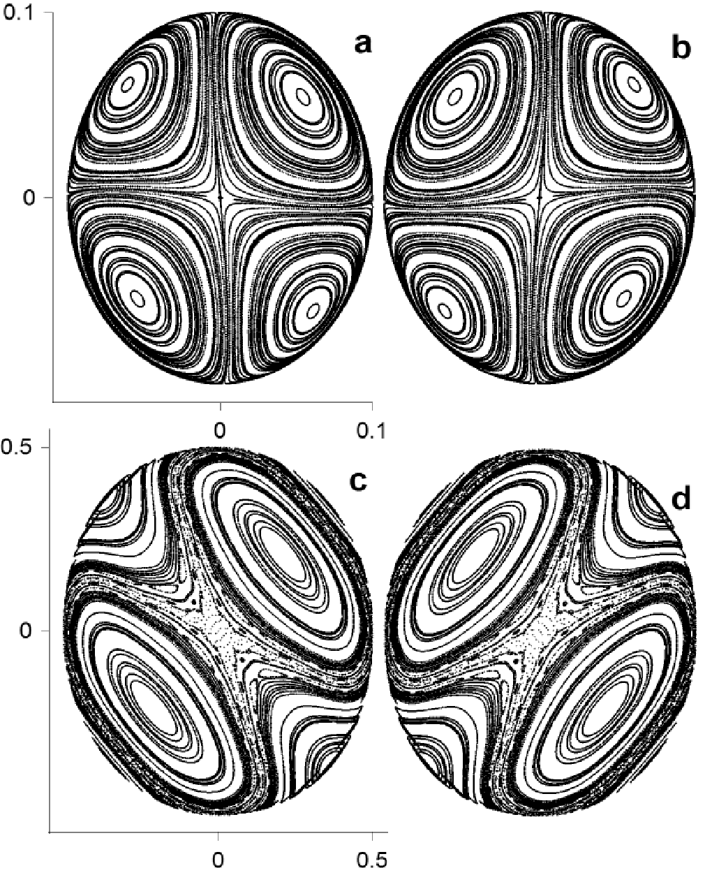
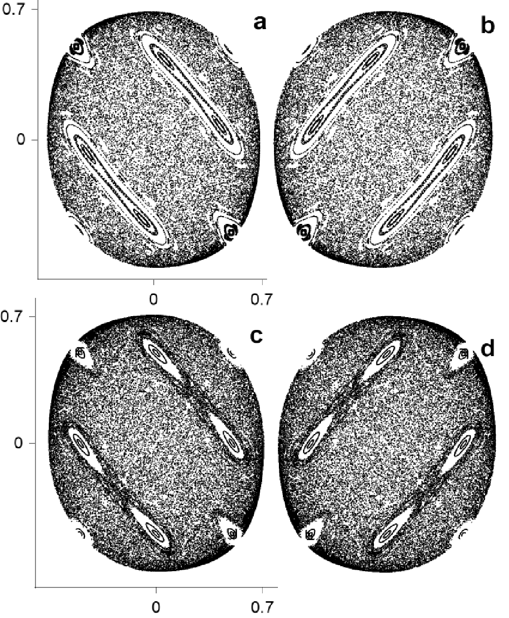
The value of the invariant is obtained by substitution of the initial condition in the generic expression of . It also follows from Eq. (20) that . In Fig. 1 and Fig. 2 we show a sequence of Poincare sections of the trace map in the plane for increasing values of . This sequence shows that the size of the sections grows with the value of the invariant . As the invariant surface has the topology of a sphere we represent separately both hemispheres corresponding to positive and negative values of . The typical orbits of the map are presented over both hemispheres. For each value of the left (right) figure is the back (front) hemisphere. Both hemispheres look similar, as if there existed a symmetry operation between them. Each hemisphere presents several axes of symmetry and some elliptic and hyperbolic points.
In Fig. 1,a,b for there appear to be no chaotic regions for the scale shown. It is easy to identify four elliptic points and one hyperbolic point with different winding numbers. Therefore, for values of near there appears to be a second integral of the motion, at least to the accuracy of these plots, and the system seems to be integrable.
In Fig. 1,c,d for , the largest resonances are clearly seen, but some of the periodic orbits are pushed to the periphery. The neighborhood of the central hyperbolic fixed point begins to be chaotic but the plot is still dominated by the KAM tori.
In Fig. 2,a,b for , the central hyperbolic fixed point has a chaotic sea but there are still some elliptic points stretching diagonally.
Fig. 2,c,d for , is similar to the previous case but now the each elliptic zone breaks into two pieces and the chaotic sea increases.
It is interesting to study the trace map when , and then . As showed in Fig. 3 the second integral of motion appears to have been totally destroyed and the integrability of the system is lost. In this case the invariant surface has two accumulation points. In the other extreme, when , the solution of the trace map is only one point.
For intermediate values of chaos sets in and large regions contain a chaotic sea of trajectories. There is no way to predict the future evolution of a trajectory in these regions, but it is possible to use the techniques of stochastic theory to determine the statistical behavior of trajectories. If no stable islands or cantori exist, the diffusion process is like that found in simple Brownian motion. However, if stable islands and cantori exist, the diffusion process becomes much complex. Here we see that there are many stable islands embedded in the chaotic region. The darker shading of trajectories along some lines indicate that these regions are bracketed by cantori. During the wandering in the chaotic sea the trajectory could get trapped in the neighborhood of a stable island for arbitrary lengths of time. The trapping of trajectories by the stable islands gives rise to power-law decay of trajectory correlations rather than exponential decays as would be expected for a purely random diffusion process. Sutherland [12] has computed the correlation function for the trace map.

Our equations are the same as in Ref. [12], but our initial conditions are chosen obeying the initial conditions of the Fibonacci QW. In both models: i)the identification of the most obvious elliptic and hyperbolic -cycles are similar, ii) he relation between the rotation of the standard alignment and the -cycles of the trace map are common, iii) the trace map dynamics determines the rotation dynamics. Therefore we can translate the results of the Sutherland model to the Fourier transform of the Fibonacci QW. Then, here also three regions of the parameter space are characterized by the qualitative differences in the decay of the time correlations. These regions are: i) near a stable elliptic cycle where the decay is slower than a power of time. ii) near a hyperbolic cycle where the decay is a power of time. iii) in the chaotic region where the decay is faster than a power of time.
IV Conclusion
In this work, we have established a trace map for the Fibonacci QW. This map has an integral of the motion that determines a three dimensional surface where the trajectories lie. The trajectories depend on the parameter , when this parameter goes to the system is integrable, but when it goes to the trajectories become chaotic. For intermediate values of the trajectories have a rich behavior where it is possible to see on the plane elliptic orbits, hyperbolic orbits, KAM tori, cantorus, etc. It is in this zone where the autocorrelation function has a time power-law dependence. This deviation from exponential decay appears because the stable islands in the chaotic sea can trap trajectories for long intervals of time. This stickiness of the islands seems to be due to a network of cantori and higher order stable islands chains which surround the stable islands and extend into the chaotic sea. It is possible to show, as in Ref. [17], that the sub-ballistic increase in the variance of the Fibonacci QW is a direct consequence of the coherence of the quantum evolution. Then, not all the trajectories of the trace map contribute with the same weight in the Fourier antitransformation of Eqs. (7,8). The more regular behavior has more weight than the chaotic trajectories and this leads to the power-law decay. Therefore, the power-law behavior in the trace map affects the wave function in such a way to obtain the sub-ballistic behavior of the standard deviation. However, it is clear that more work will be necessary to understand these mechanism more deeply.
V Acknowledgments
I thank V. Micenmacher for his comments and stimulating discussions. I acknowledge support from PEDECIBA and PDT S/C/IF/54/5.
References
- [1] J. Kempe, Contem. Phys., 44, 307 (2003); also in quant-ph/0303081.
- [2] Y. Aharonov, L. Davidovich and N. Zagury, Phys. Rev. A 48, 1687 (1993).
- [3] S. Godoy and S. Fujita, J. Chem. Phys., 97, 5148 (1992).
- [4] V. Kendon, quant-ph/0606016 (2006)
- [5] P. Ribeiro, P. Milman, and R. Mosseri, Phys. Rev. Lett. 93, 190503 (2004).
- [6] A. Romanelli, R. Siri, and V. Micenmacher, Phys. Rev. E 76, 037202 (2007)
- [7] A. Romanelli, Phys. Rev. A 76, 054306 (2007)
- [8] P. Lévy, Theorie de l’Addition de Variables Aleatoires, (Gauthier-Villiars, Paris, 1937)
- [9] A. Romanelli, A. Auyuanet, R. Siri, and V. Micenmacher, Phys. Lett. A 365, 200 (2007).
- [10] S. Abe and H. Hiramoto, Phys. Rev. A 36, 5349 (1987)
- [11] J.X. Zhong and R. Mosseri, J. Phys. Condens. Matter 7, 8383 (1995)
- [12] B. Sutherland, Phys. Rev. Lett. 57, 770 (1986).
- [13] M. Kohmoto, L.P. Kadanoff, C. Tang, Phys. Rev. Lett. 50, 1870 (1983).
- [14] A. Nayak and A. Vishwanath, e-print arXiv:quant-ph/0010117
- [15] B. Tregenna, W. Flanagan, R. Maile and V. Kendon, New J. Phys. 5 83 (2003).
- [16] E. Bach, S. Coppersmith, M. Paz Goldschen, and R. Joynt, e-print arXiv:quant-ph/0207008.
- [17] A. Romanelli, A. C. Sicardi Schifino, R. Siri, G. Abal, A. Auyuanet, and R. Donangelo, Physica A 338, 395 (2004).