Reconstruction of eye movements during blinks
Abstract
In eye movement research in reading, the amount of data plays a crucial role for the validation of results. A methodological problem for the analysis of the eye movement in reading are blinks, when readers close their eyes. Blinking rate increases with increasing reading time, resulting in high data losses, especially for older adults or reading impaired subjects. We present a method, based on the symbolic sequence dynamics of the eye movements, that reconstructs the horizontal position of the eyes while the reader blinks. The method makes use of an observed fact that the movements of the eyes before closing or after opening contain information about the eyes movements during blinks. Test results indicate that our reconstruction method is superior to methods that use simpler interpolation approaches. In addition, analyses of the reconstructed data show no significant deviation from the usual behavior observed in readers.
I Introduction
Studies of eye movements have revealed enormous insights into the understanding of cognitive processes during visual search, scene viewing and reading. The development of high resolution techniques that allow researchers to record the eye movements online during experiments constitute the base for the research in this field. Systems range from coil systems, Electro-Oculo-Graphy EOG systems and video based systems (e.g. Eyelink) to systems using infrared light to capture the pupils movements, such as the Dual Purkinje, corneal reflection and pupil boundary systems. All of those systems require that the reader’s eyes are open and closing the eyes inescapably means loss of data measurement. A typical and natural closure of the eyes is the blink, a brief closing of the eyelids. Blinks can occur spontaneously, as a normal periodic closing (e.g. for eye lubrication), reflexively (protective, e.g. due to an air puff or an object moving towards the eyes) and voluntarily (e.g. by command) [1]. In this work, we propose a method, based on the symbolic sequence dynamics of the eye movements, to reconstruct the eye positions during blinks in a reading experiment, in which readers were instructed to read 144 isolated sentences of the Potsdam Sentence Corpus (PSC). The main assumption behind this approach, for reconstructing the eyes position during a blink, is that the eyes movements before and after a blink occurs carry information about how the eyes behave during a blink.
In reading research, we distinguish between saccades, rapid eye movements of the eyes with high velocities, and fixations, when our eyes remain relatively still between the saccades. The function of a saccade during reading text is to bring a new text section into foveal vision, where visual acuity is highest.
Two important questions arise when the reader closes his eyes. Did the reader make a saccade ? If the reader did make a saccade, at what time did the saccade start? The exact starting time of a saccade is crucial for the detection of fixations and influences fixation durations. The later the saccade happened during a blink, the longer will be the detected fixation prior to the blink. Fixation duration is the primary measure related to cognitive processes during reading comprehension.
One approach to treat the reading data with blinks is to exclude the trials during which blinks occur. A trial includes the recording of the eye positions while reading a given sentence. A different approach would be to analyze the trial up to the point in time when a blink occurred. Both approaches might exclude relevant information concerning the particular dynamics of eye movements in reading and blink phases. Therefore, it would be of high value to the data analysis in reading research, especially in data sets of older readers, to reconstruct a complete sequence of saccades and fixations per trial.
If the reader did not make a saccade while the eyes were closed, then the eyes have not moved during the blink and their position before and after the blinking is roughly the same. The problem appears when a saccade happens during a blink and the challenge is to accurately reconstruct such a saccade.
The first difficulty in treating eye movement data is provided by its clear non-stationarity characteristic (see Sec. II), mainly caused by the reader’s goal to read the sentence which commands the spontaneous dynamics of the eyes composed by the alternation between (micro)saccades [2] and fixations. In addition, once that the reader decides to make a saccade, there is a random time-delay until the moment the saccade is actually realized (see Ref. [3]). So, the movement of the eyes is not only non-stationary but also contains stochastic components. These characteristics together unable one to model the eyes positions by the usual time-delay reconstructing technique [4].
The second difficulty is the fact that the eyes’ dynamics is the result of a typical complex system [5], a system whose output is produced by the interaction of many systems, which presumably has a high-dimensional output. In fact, on the one hand, the long-term evolution of the eyes movements have a high-dimensional character, which calls for some kind of stochastic model [6]. On the other hand, the short-term evolution of the eye movements possess a dynamic typical of low-dimensional systems, in particular a saccade.
In order to resolve the first difficulty, instead of working with the eye position, we work with the eye velocity (see Sec. IV). The velocity is the most simple technique to transform a non-stationary data into a stationary one. This technique is often used to treat complex data. Among the many works, this technique was used in the analysis of microsaccades (rapid eyes movements) [7], stock market fluctuations [8], and plasma turbulence [9].
To resolve the second difficulty, we make models that consider the dual low-high-dimensional characteristic of the eye movements. First, we model the short-term evolution of the eye oscillations, in particular a saccade, using a low-dimensional system, a one-dimensional damped oscillator (see Sec. III). The main parameters that adjust this oscillator to saccades, the period and the damping coefficient, are obtained from both the low and high dimensional characteristics of the eye movements.
For the purpose of finding such parameters we use a technique suitable for treating complex data, the symbolic dynamics [5, 10]. A complex system with infinite number of possible output values, in particular the eye velocities, is transformed into a much simpler system by encoding their velocities using a few number of letters, creating the symbolic sequences (see Sec. IV). In this work, we consider symbolic sequences composed of 4 letters.
The symbolic dynamics technique has a powerful property that can be explored to treat systems that possess different dynamics for different time-scales. A short-length symbolic sequence generated from short-term time intervals provides an instantaneous visualization of the movement of the eyes, while a large-length symbolic sequence generated from long-term time intervals might reveal stochastic properties [11] of the eye movements, averages, and other quantities. Stochastic properties can also be obtained by producing averages of many short-length symbolic sequences. These properties are fundamental to the success of our reconstruction method.
In order to know whether and when a saccade happens, during a blink, we consider symbolic sequences created by encoding the eye velocities before and after this blink occurs (see Secs. IV and V). To know whether a saccade happens, we compare the probabilities of finding certain groups of short-length symbolic sequences before and after this blink, with the probabilities of finding those short-length symbolic sequences before and after all saccades observed during all the trials in an experiment. At this point, we take advantage of the statistical character of short-length symbolic sequences. To know when a saccade happens, we search in the large-length symbolic sequences particular repeating sequences of letters that correspond to the encodings of oscillations that the eyes make before or after making a saccade.
Notice that an experiment is composed of many trials. In addition, the dynamics of the eyes is highly influenced by what is being read, and besides during an experiment the participant makes a series of blinks. As a consequence, we cannot construct infinity large symbolic sequences, but symbolic sequences with a finite length smaller than . Further, we decompose these sequences in even smaller sequences regarded as words.
We define in the following way: Symbolic sequences of length larger than contain roughly the same content of information of symbolic sequences of length . So, the long-term character of the symbolic sequences is provided by finite-size symbolic sequences of length not larger than . For our experiment, is of the order of 60, which means symbolic sequences composed of 60 letters, corresponding to a time interval of 120ms (see Sec. V).
Once we have ensured that a saccade occurs during a blink and we have obtained an estimation of the time the saccade starts and its period, the time series is reconstructed by assuming that the position of the eyes before and after the occurrence of a blink can be optimally connected by a time series generated by a simple one-dimensional damped oscillator (see Sec. VIII).
In order to check if our method can really reconstruct saccades during blinks, we study its performance to reconstruct the position of the eyes during artificially created blinks. As shown in Sec. VII, our method can reconstruct saccades much better than if we had made the reconstruction assuming that a saccade happens in the middle of a blink, having a period given by the average period of all the saccades observed in all trials.
Finally, we have shown (in Sec. IX) that relevant reading measures that reflect cognitive processing are not affected by our reconstruction method, which validates our method from the psychological point of view.
In appendix A, we show the most important parameters, variables, and constants considered in this work.
II Experimental Data

Data. In this work, we consider only data from the horizontal position of the right eye, denoted by . A sample of the raw data set is shown in Figs. 1(A-B), where in pixels is plotted over time. In both figures, the typical alternation between saccades and fixations can be observed. In Fig. 1(B) we observe a data loss (the position is set to zero) due to a blink that occurred while the eyes made a saccade, indicated by the misalignment of the signal before and after the blink.
Participants. The method of reconstruction was applied on data sets of four young participants (mean age 18.5 years) and three old participants (mean age 72.3 years). All participants had normal or corrected to normal vision. Visual acuity was assessed with a standard optical chart (Landolt rings; 5 m distance). Eye movements of 26 other young participants and 22 other old participant serve as a baseline to compare gains of the reconstructed data with non reconstructed data. Each individual data set of the seven participants is identified by , with . Average number of blinks per minute for the seven subjects was 6.97 blinks/min.
Apparatus. Single sentences were presented on the center line of a 21-in. EYE-Q 650 Monitor (832 pixels x 632 pixels resolution; frame rate 75 Hz; font: regular, New Courier, 12 point) controlled by an Apple Power Macintosh G3 computer. Participants were seated in front of the monitor with the head positioned on a chin rest. Eye movements were recorded with an EyeLink II system (SR Research, Toronto) with a = 2 ms sampling rate. All recordings and calibrations were binocular.
III Dynamics of the saccade
Two typical saccades are shown in Figs. 2(A-B) in black solid line. In (A), the position of the right eye moves to the right, making a rightward saccade, while in (B), the eye moves to the left, making a leftward saccade. A saccade begins at time if , for and . The period of the saccade is determined by checking if changes the signal once, for . So, ms. The final position of the eye after a saccade, the beginning of a fixation happens for the time if for , the signal of changes three times. While reading all the sentences a participant makes saccades. Each saccade can be identified by the following parameters , with , where is the amplitude of the saccade , being and . These quantities are represented in Fig. 2(A).
We model the dynamics of the horizontal position of the eye during a saccade in the same way eyelid saccades were modeled in Ref. [13], using a damped oscillator described by
| (1) |
with = and =0. Equation (1) can describe a saccade in the coordinate system of the eye position , for the saccade , if the following transformation is applied
| (2) |
The time in Eq. (1) is transformed to the time of the experiment by
| (3) |

The saccades are modeled by Eq. (1) with parameters (damping coefficient) and (angular frequency of the saccade oscillation) such that this equation describes a supercritical damped harmonic oscillator. This hypothesis is sustained by the fact that most of the time . However, in 10 of the saccades we find that or is slightly bigger than , which violates this hypothesis. For a more general model for saccades one could use the dynamical system proposed in Ref. [14]. However, for the scope of the present work, Eq. (1) is a sufficiently good model for a saccade. Note that if that usually implies that is small and therefore, for a short time interval the saccade can be well approximated by the supercritical model which produces almost a straight line. In addition, the effect of this small saccade in the data treatment is small. Then, for the saccade , we assume that
| (4) |
and
| (5) |
In conclusion, a saccade can be uniquely defined by the following minimal set of three parameters . Using the obtained minimal set of parameters, we model the saccades of Figs. 2(A-B) using Eqs. (1), (2), and (3). The model qualitatively reproduces the real data, as can be seen in Figs. 2(A-B). During a blink, however, in case a saccade happens, and are undetermined and will be estimated by searching for special patterns in the symbolic encoding of the eye velocities of time series before and after the occurrence of a blink.
IV Symbolic characterization of the eye dynamics
One of the most efficient techniques to turn a non-stationary data set into a stationary set is to work with the velocity space, instead of using the phase space. The velocity of the eye is given by , which will be denoted by . The velocity is still a very complex variable. To reduce its complexity without compromising its content of information, we symbolize the data series using a small-size alphabet composed of 4 letters: .
The velocity space, a first returning map of the velocity variable, is shown in Fig. 3(A). Points in the horizontal axis represent the relation between the velocity at the ”time” [, in units of ms] and in the vertical axis, the velocity at time []. In this figure, we plot the velocity space for all short time series (ms) before a saccade begins, at the time . That is, we consider the time interval . In Fig. 3(B), we plot the velocity space for all short time series (ms) right after the saccade reaches its maximum, at the time . So we consider the time interval . Notice that there is a clear visual difference between both velocity spaces, which reflects a difference in the eye movements before and after saccades happen.
The symbolic encoding of the velocity variable is done by first splitting the velocity space in the four partitions as represented by the dashed lines in Fig. 3(A-B), and then assigning letters if the velocity trajectory is within one of these partitions: if and , we encode this point by a ’0’; if and , we encode this point by a ’1’; if and , we encode this point by a ’2’; if and , we encode this point by a ’3’. Thus, a trajectory with points is encoded into a symbolic sequence with letters, regarded as , with =. is assumed to be an even number, so we can easily split the symbolic sequences into two non-overlapping sequences.
For the visualization of the symbolic sequences, we split them into two non-overlapping words of letters, and encode these two words into two real numbers and by the following rule
| (6) |
Then, we plot the numbers versus .

The existence of blinks together with the fact that sentences have a limited number of symbolic sequences, and further the fact that an experiment consists of many trials unable one to consider longer symbolic sequences. Instead, we work with symbolic sequences of length smaller than . These symbolic sequences are constructed in a way to reflect some particular characteristic of the eye movements.
In this work, we consider the following types of symbolic sequences: The length- symbolic sequences, , and are constructed using the encoding of the eye movements before the saccade starts (time interval ) and after this saccade ends (time interval ), respectively. The symbolic spaces of are shown in Fig. 3(C-D), which are the symbolic spaces of the velocity spaces of Figs. 3(A-B), respectively. They show a clear mismatch between the eye movements before and after saccades happen. The length- symbolic sequences, denoted by and , are constructed by the encoding of the eyes velocities before and after a blink that happens at the time ms.
Finally, we define the symbolic sequences relative to the saccade in the following way. For a fixed , we construct non-overlapping words of length , with , from the velocity variable, for all valid trials, i.e. all time intervals of the experiment where blinks are absent and where there is no interruption of the reading due to the beginning or ending of the sentences. Then, the symbolic sequences are all symbolic sequences formed by 3 pairs of length- words in the form , such that a saccade happens during the time at which was generated. The symbolic space for participant , denoted by , is constructed by converting the pairs of words ,, , , and , into pairs of real numbers using Eqs. (6). The symbolic space represents the pair of words and represents the pair of words . These symbolic spaces for a participant are shown in Figs. 6(A-C).
The rules that describe the way short-length words appear after short-length words in the pre and post saccades symbolic sequences [ and , respectively], also know as the grammar, is described by the digrams that give the possible transitions and probability of transitions between words of letters. For a given , with , we split the symbolic sequence in a sequence of non-overlapping words of length , and analyze their probability transitions. Given a symbolic sequence composed by letters, with , we generate the words, regarded as , each of length . As an example, for =2, given a sequence we create the sequence =, with = and =. The probability of having a length- word followed by is represented by .
Taking participant as an example, for =1, the digram for the one-word letters in the pre-saccade symbolic sequences, , (with =24 symbols) is shown in 4(A), and for the post-saccade symbolic sequences, , in Fig. 4(B). We only show the most different probability transitions.
For example, the probability of finding a ’0’ that is followed by a ’0’ in the pre-saccade symbolic sequences is 0.13 while it is 0.27 in the post-saccade symbolic sequence. The discrepancy might be a combined effect due to many factors. The damping of the eye movements after the saccade (after the period ) results in smaller amplitudes and slower oscillations in the eye movements, reflected in symbolic sequences that present more length-2 sequences of zeros (positive velocity) as well as more length-2 sequences of twos (negative velocity). Note, however, that in the long term, does not present large repeating sequences of zeros or twos, because it reflects the dynamics of the fixations, when the eye randomly oscillates around a fixed point. This causes the big empty areas in Fig. 3(C), specially within [0,0.4].
The large probability transition, , for the pre-saccade sequences is a consequence of the fact that the pre-saccade velocities change its sign more often, possibly a consequence of the fact that in the pre-saccade the eyes present faster oscillations.

It is important to notice that the digrams of length- words in the pre and post saccades symbolic sequences do not change significantly by varying in the interval ms. This means that the digram dynamics presents a sort of time invariance, if is kept constant, while varying .
In the following, we will consider in our reconstruction method =2, since for no significant better performance of the reconstruction method was obtained.
The digrams represent the statistical character of the eye movements before and after a saccade happens, provided by averages from the probabilities of many short-length words observed in all symbolic sequences . They will be used to identify whether a saccade occurs during a blink.
V Predictions based on the symbolic dynamics
As a first step, we calculate the Shannon’s entropy of the pre- and post-saccade symbolic sequences, and , of length , in order to estimate an upper bound for the time interval so that predictions can be made by using the information contained in these symbolic sequences
| (7) |
where represents the probability of finding a particular symbolic sequence composed of letters.

In Fig. 5(A), we show for participant , which is an estimation of the amount of information for the symbolic sequences and , for all saccades of the experiment. Empty circles show the entropy of the sequences , and empty squares show the entropy of the sequences . An important point that can be derived from the shape of this curve is that the maximum entropy values for both sequences is approximately equal. The maximum of the entropy is reached when , with defined as
Thus, once the time interval provides sequences for which the maximum of the entropy is reached, an increase in the the length of the symbolic sequences does not increase the content of information.
However, these maxima are reached for different . This becomes clear in Figs. 5(B-C). In (B), the value of the time interval , when the maximum value is reached for each one of the participants, is shown. Clearly, the maximum of the entropy is reached for shorter time in than in . The time intervals in (B) give an estimate of the time length one can still extract relevant information from the symbolic sequences, i.e., an estimation of the value of . The presence of a maximum for the entropy is a result of either under-sampling or the presence of correlations in the data set. That also reflects that our data is composed by a finite number of ”repeating” trials that last for a finite time. In (C), the maximum of the entropy is visualized.
As a second step, in order to derive predictions from symbolic sequences, we have to assume that a certain degree of dynamical constraint exists in the data, and that words are dynamically connected to words that appear previously. Given for example the following symbolic sequence: “3 3 1 2 3 0 . 0 1 3 1 3 0 . . . 2 2 3 0 0 0 . 1 3 3 1 2 2”, with and representing two words with 6 letters, we expect that can be derived from the two words that precedes it, denoted by =”3 3 1 2 3 0” and =”0 1 3 1 3 0”, and can be predicted from the two words that appear after it, denoted by =”2 2 3 0 0 0” and =”1 3 3 1 2 2”.
The eye movements can be reduced to two main types of behaviors: Saccades and fixations. Since fixation is approximately constant and could be modeled by a zero velocity behavior, for the purpose of the present work, the only relevant behavior to be predicted in the sequences is the occurrence of a saccade.
Throughout this paper we make two more fundamental assumptions.
- Assumption I
-
A saccade is likely to occur within the time interval that creates the sequence [] if the digrams of the pre-saccade [post-saccade] symbolic sequences is likely to be a generator for the word pairs . [.].
Likelihood to be a generator depends on a defined probabilistic measure. We define the quantity
| (8) |
In this equation, represents a pair of length-2 words (=2) observed either in . or .. The probability of finding followed by in the digrams of either the pre or post-saccade symbolic sequences is denoted by . That generates the quantities and , respectively.
A saccade is likely to have happened during the time at which was generated if . The idea here is that if in the word pair , the digram that represents the pre-saccade dynamics likely describes the dynamics that generated this pair. That is, a saccade is likely to have happened during the time at which was generated. So, Eq. (8) is a probabilistic distance of how the dynamics of the pre or post-saccade (given by the digrams) conforms with either the word pairs or .
The occurrence of a saccade time is consider to be undetermined if one of the following conditions apply: (i) for at least one sequence in both and , we find that and ; (ii) defining the probabilistic distance between the digrams of the pre-saccade and post-saccade sequences as
| (9) |
we find that .

- Assumption II
-
can be approximately obtained by applying a transformation into and . We denote the resulting reconstructed space by .
The result of the transformation is shown in Fig. 6(D), where we plot the symbolic sequences of the form , which produces the following pair of points , , , , . Therefore, the transformation results in = and =. Note the similarity between the space in (A) and the space in (D). This can also be seen in Fig. 7, where we show the probability distribution of points in the horizontal coordinates of the spaces in Figs. 6.

The chosen transformation is one of many other possible dynamics from which one can successfully recover an equivalent space. But, we choose it because symbolic sequences of the desired form are often observed in some of the sequences . These symbolic sequences are encoded into real sequences [using Eq. (6)] into . Then, we search sequences of pairs of words in the symbolic sequence of the saccade, , whose real encoding sequence regarded as is denoted by ....., with = and =. We find that the percentage of points , that respects this rule follows a power-law with respect to , , as shown in Fig. 8, which implies that .
Therefore, even if we decrease , there is still a finite probability, larger than if the relation between and were linear, of finding sequences as the ones created by the transformation . So, symbolic sequences similar to the desired one appear often, which also means that points in the symbolic space return often to the diagonal.
One should expect that if the symbolic sequences were generated by a Markov Process. If the probability of having a symbol ’0’ is and of having a ’1’ is , the probability of having the symbol ’0’ followed by ’1’ in a Markov process is given by . In fact, the found power-law is an effect of the existence of certain constraints in the eye’s movements, a typical characteristic of dynamical systems.
The interpretation of the chosen transformation is simple: The dynamics of the eyes for short-time intervals before and after making a saccade reveals if a saccade will happen or has already happened.
The main difference between the symbolic space and is the absence (in ) of large sequential sequences of zeros or twos, as the ones observed in . That is easy to be understood by considering that similarly to what happens in the space for the symbolic sequences [see Fig. 3(D)], represents the long term behavior of the eyes during a fixation, which have roughly a constant velocity, and does not present tendencies which would be encoded by larger sequences of zeros or twos.
Another point that is relevant to be emphasized is that before a saccade happens our eyes have an excited dynamics ( in Eq. (4) is negative), while after the saccade happens the eyes have a dissipative (damped) dynamics ( in Eq. (4) is positive). The damping effect is also another reason for the absence of relevant tendencial movements.
Thus, can be considered to represent the autonomous dynamics of the eyes, while represents the forced dynamics. The force is produced by the will of the participant to move its eyes. Recall that the saccades are reconstructed only considering the dissipative dynamics in the super-critical behavior.

VI Approaches for reconstructing the blinks
A participant makes blinks during the reading and a blink occurs at the time (in units of , or ms), lasting (in units of or ms), with . As introduced in Sec. IV, we represent the length- symbolic sequences that appear before the participant blinks by a pair of length words , and the length- symbolic sequences that appear after the participant opens the eyes is represented by . Based on assumption II, the reconstructed symbolic dynamics of the blink is given by .
Then we adopt a series of procedures. First, we check whether () is likely to be generated by the digrams of the pre-saccade (post-saccade). In other words, we detect equivalence of with the pre-saccade digram (assumption I). This suggests that a saccade might have happened right after the participant blinks, which would imply that in one would find sequences of either zeros (’0’), if the eyes move to the right after blinking or twos (’2’), if the eyes move to the left.
If we find a word composed of at least 4 [15] sequential zeros followed one after the other (or twos) in , we assume a saccade must have happened in the time ms, where is a function of the number of letters that precedes the largest sequential sequence of zeros (or twos) in , denoted by . Similarly, we assume that the period of the reconstructed saccade in units of , denoted by , is proportional to the number of sequential zeros (or twos), denoted by .
If we detect equivalence of with the digram of the post-saccade, we assume that the saccade must have started in the time ms, where now depends on the number of letters that appear before the sequential sequences of zeros (or twos) in . The number of sequential zeros or twos gives the value from which one can calculate the period of the saccade.
In the case a saccade is likely to have happened during a blink, but no sequence of only zeros or twos are found either in or that have at least length 4, then, we look for sequences in the whole reconstructed sequence . We also search for a sequence of zeros or twos in the whole reconstructed sequence if the occurrence of a saccade is undetermined.
In the following section we show how to choose the value of in order to improve the performance of our reconstruction method. However, while is considered to be fixed, the -th blink has a period which is, in general, different than . If the word pairs and show evidence that a saccade happens during the blink, from the previous considerations this blink will be reconstructed by assuming that the encoding symbolic sequence of the blink is given by . Saccades are reconstructed by finding the repeating sequences of zeros or twos in , , or . However, the time interval of the blink () is different than the time interval associated with () as well as the half-time interval of the blink is different than the time interval associated with either or ().
Therefore, if we find that the period of the saccade is (in units of ), we rescale this time interval with respect to the time interval of the blink, and consider that the saccade during the blink has a period given by
| (10) |
Similarly, the time at which the saccade is assumed to have started is calculated from which is given by
| (11) |
Equations (10) and (11) are constructed under a reasonable hypothesis that the time scale of the eye movements during a blink are influenced by the period of the blink. They also adjust the time interval of the reconstructed symbolic sequences to correspond to the period of the blink.
If no words composed of at least 4 zeros (or twos) are found in , we assume that a saccade happens in the middle of the blink and the average period of all saccades during reading is taken as the period of the saccade. If Eqs. (10) and (11) results in , we make .
Once we have worked out the time that the reconstructed saccade starts, , and the period of the saccade , we assume in Eq. (1) that , where =, with representing the position of the eye after opening (in the end of the -th blink) and representing the position of the eye right before closing. , in Eq. (3), should be substituted by . We also assume that after a time given by , the reconstructed position of the eyes from Eq. (2) is a value so that =1 pixel. This means that after 2.5 oscillation periods, the reconstructed saccade is supposed to end. From this hypothesis, we can calculate the quantity , which is used to calculate , in Eq. (4).
VII Optimal parameters, robustness, and statistical significance of the reconstruction method
To validate our method, we reconstruct blinks artificially created around the places where saccades happen. So, for each one of the saccades made while reading, we create a series of =10 blinks that last for a time interval . The first artificial blink ends at the time ms (middle of the saccade) and the last artificial blink begins at this same time ms. Thus, each artificial blink, referred to as , with starts at the time :
| (12) |
The reconstruction of the artificial blink uses our method previously described (Secs. III, IV, V, and VI). We first constructed the digrams, using the symbolic sequences of length , generated from the whole data series, without the presence of artificial blinks. Then, for every artificial blink we generate the symbolic sequences and as described in Sec. IV and VI.
After applying our method, for every artificial blink around a saccade , we find that the reconstructed saccade starts at the time (in units of ms) and has a period (in units of ms).

An example of the reconstruction of an artificial blink for the participant is shown in Fig. 9, indicated by the empty circles. For this saccade, we have detected that the symbolic sequence of the post-blink, , was likely generated by the digram of the post-saccade. Remarkably, indeed, the saccade happens right before the end of the artificial blink. Notice that after the artificial blink ends, one notes a slight movement of the eyes to the right (increasing the value of ), caused by the typical oscillatory behavior after the saccade happens. This oscillatory behavior produces in the symbolic sequence, , the sequential sequences of zeros and twos from which we obtain the time at which the reconstructed saccade begins [] and the period of the reconstructed saccade [] within an artificial blink.
To quantify how good is the reconstruction of the artificial blink, we calculate the absolute difference between the predicted time for the beginning of the saccade, , and the real time for the beginning of the saccade, , normalized by the time interval of the artificial blink. We calculate this quantity for all the artificial blinks and average it, producing
| (13) |
Then, we calculate the absolute difference between the real time when the saccade starts, , and the time of a hypothetical reconstructed saccade if it had started in the middle of the artificial blink, normalized by the assumed time interval of the artifical blink:
| (14) |
where =+.
Similarly, we calculate the absolute difference between the period of the reconstructed saccade, , and the real period , normalized by the average period of the saccades, producing
| (15) |
and we calculate the absolute difference between the real period of the saccade, , and the period of a hypothetical reconstructed saccade if it had been reconstructed assuming that it is equal to the average period of the saccades , producing
| (16) |
Our method produces statistically significant results if the quantities
| (17) |
and
| (18) |
are positive. Notice that a positive is a measure of ’how much better our method reconstructs the time a saccade happens’ if compared to a method that would reconstruct a saccade as if it had happened in the middle of the artificial blink. A positive is a measure of ’how much better the method reconstructs the period of the saccade’.
We calculate these quantities by considering different values of the time interval considered for the artifical blink. For each value of , we reconstruct the artificial blinks using symbolic sequences of different lengths . In Figs. 10 and 11, we show and , respectively, for an young participant. In Fig. 12 and 13, we show the same quantities for an old participant.


These figures illustrate that there is an extended region in the parameter space where parameters can be changed and still our method reconstructs the saccades present in the artificial blinks in a better way than if we had just guessed that the saccade starts in the middle of the artificial blink, having a period equal to the average period of all the saccades while reading. This demonstrates the robustness of prediction of this method, under a wide range of and values. Similar positive results for the blink reconstruction were obtained for the other participants.
The quantities and depend more on the length of the symbolic sequences, , than on . This indicates that our method is able to reconstruct real blinks, whose durations extend over a wide range, well enough, if is well chosen. Roughly, should produce good results.
In table 1, for each participant the average duration of the blinks is listed in the second column, the average period of the saccades in the third column . The value of that produces the largest value of and are shown in the columns 4 and 5, respectively. We consider ms, a time interval for which we can extract relevant information from the symbolic sequences (see Sec. V). Thus, a reconstructed artificial blink that reproduces well the time of the beginning of the saccade is obtained by using shown in the fourth column. On the other hand, a reconstructed artificial blink that reproduces well the period of the saccade is obtained by using values shown in the fifth column. This shows a kind of Heisenberg’s principle in our method. Either one reconstructs reasonably the time a saccade starts or its period, but not both quantities simultaneously, except for the readers and .
Other quantities that characterize the participants are also shown in this table. These are the probabilities (column 6) of finding that the pre-blink symbolic sequences, , (using a value from the fourth column) were likely generated by the digram of the pre-saccades dynamics, the number of blinks per second (column 7), the average angular frequency with which the reader makes a saccade (column 8), the average damping coefficient of the saccades (column 9), and the time that the participants took to read all the sentences of the PSC, the quantity (column 10).
It is interesting to note that participant has a high probability (0.737) of making saccades immediately after closing the eyes. Furthermore, the time he takes to read all the sentences of the PSC is the shortest compared to the other participants. This suggests some sort of efficient reading behavior in the sense that the saccade target is already detected before the reader blinks.
Note that for many participants the ideal value of that better reconstructs the time at which a saccade starts is of the order of the time interval at which we can still extract relevant information from the symbolic sequences (see Sec. V).
| (ms) | (ms) | (ms) | (ms) | pre-blink | blinks/s | T (s) | |||
| 60.000 | 41.485 | 120 | 116 | 0.737 | 0.134 | 0.133 | 0.104 | 788.928 | |
| 75.766 | 35.991 | 76 | 116 | 0.333 | 0.134 | 0.102 | 0.080 | 1149.148 | |
| 48.424 | 40.045 | 120 | 116 | 0.060 | 0.030 | 0.137 | 0.107 | 1110.560 | |
| 53.289 | 33.198 | 72 | 116 | 0.000 | 0.046 | 0.118 | 0.093 | 968.500 | |
| 98.280 | 26.034 | 76 | 116 | 0.236 | 0.098 | 0.185 | 0.099 | 1021.836 | |
| 72.502 | 23.890 | 76 | 116 | 0.115 | 0.344 | 0.177 | 0.101 | 954.918 | |
| 72.545 | 23.905 | 92 | 116 | 0.125 | 0.027 | 0.184 | 0.113 | 817.594 |
VIII Reconstructing the blinks
For reconstructing the real blinks, we consider =2 and from the column 4 of Table 1, which might allow our method to reconstruct well the time at which a saccade starts. We consider symbolic sequences and , that encode the eye velocity before and after a blink, respectively. In Figs. 14(A-D), we show a few examples of the blink reconstruction for the participant . In (A), was found to be likely generated by the digram of the pre-saccade symbolic sequence. In (B), two blink reconstructions are shown. In the first blink, the method is unable to determine if a saccade happens during this blink and it is assumed that a blink happens in the middle of the interval. In the second blink, was found to be likely generated by the digram of the post-saccade, which means that a saccade must have started right before the eyes open, the same case is illustrated in (C). In (D), was found to be likely generated by the digram of the pre-saccade.

IX Analyses of the reconstructed data
The results of the statistical tests provided in Sec. VII and the reconstruction examples in Sec. VIII indicate that the model reconstructs the data losses due to blinks with qualitatively high precision, and the reconstructed data seem to reproduce the natural movement of the eyes. Of further interest is the benefit we gain from the reconstruction procedure for the analysis of eye movements in reading.
We have analyzed the reconstructed data using several eye movement measures, that are considered to be related to cognitive processing during reading, when the word is the unit of analysis [16]. Gaze duration is defined as the sum of all fixations on a word in first pass reading. Total reading time is the sum of all fixation durations on a word, including regressions from second pass reading. First pass single fixation duration describes the fixation duration when a word is fixated exactly once, preceeded and followed by a forward saccade. If a word is fixated once, fixation position in the word is usually in the first half of the word, that is on the second or third letter of a word [17]. The skipping rate is the probability a word is not fixated during the first inspection of the sentence, whereas regression probability is here defined as the chance that a word is the origin of a regressive eye movement. All of these measures are important variables if the ease of processing, strategies during reading, or effects of the material on fixational behavior (e.g. word frequency effects) are of theoretical interest.
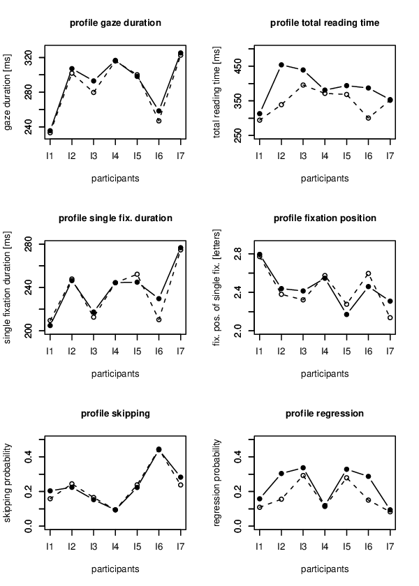
In Figure 15 means in total reading time per word, gaze duration, first pass single fixation duration, fixation position of single fixations, skipping, and regression probability for the data of the seven participants with and without reconstruction are visualized. Despite individual differences in eye movement patterns, there are no significant changes between the original data set and the reconstructed data for any of the six processing measures. In fact, the qualitative similarity of the data with and without reconstruction in the various measures of reading behavior is quite impressive.
Participant and show the largest differences in total reading time and the probability of regressions. Since the probability of blinking increases with reading time, i.e. second pass reading, and trials with blinks were excluded from the analysis in the data without reconstruction, it is plausible that the valid trials of these two subjects in the data without reconstruction mostly include trials with few second pass fixations. Total reading time and the number of regressions depend on second pass reading; in fact, total reading time correlates with the number of regressions, since second pass fixation durations are included in total reading time. Therefore, longer total reading times and higher regression probabilities for these two subjects in the data with reconstruction is not surprising, but highly expectable.
X Conclusions
We have used the symbolic representation of the eye velocities as a tool to reconstruct an eye movement signal obtained in a reading experiment, when the eyes are closed during a blink. The dynamics of saccades played a crucial role for predicting the signal of the eye positions during blinking. Essentially, for each participant the signal could be restored by finding the closest similarities between the dynamics of the eye velocities before or after a saccade and before or after a blink. Thus, the eye movements before and after a blink occurs carry information about how the eye behaves during a blink. Results demonstrated a qualitatively precise prediction for the signals during blinks.
The reconstructed data did not affect eye movement measures related to cognitive processing during reading. Total reading time, gaze duration, and single fixation duration for words did not change significantly, neither was fixation position in the word, skipping probability or regression probability affected by the reconstruction of the signal. This was true for young as well as old subjects. Especially for the analysis of processing measure including second pass reading (e.g. total reading time, regression probability), the reconstruction method is a valuable tool to increase statistical power. Blinks occur more frequently if reading time increases. Thus, trials containing second pass reading are relatively more often excluded from the analysis, if blink occurrence is the criteria for trial exclusion. The use of a reconstruction method recovers those trials with relatively many blinks, providing a more complete picture of the processing variances between subjects during reading. The reconstruction of saccades during spontaneous blinks from saccadic data recorded from the open eye is a useful approximation. We cannot rule out that the blink itself interferes with the motor program of the saccade, changing its parameters in subtle ways. As far as we know, at present there is no reliable evidence in support of this possibility. In sum, the described reconstruction model is a precise and useful tool to overcome problems of data loss in eye movements during reading, especially if the analyses of fixation sequences is fundamental to theoretical questions.
The method proposed here was applied to reconstruct the data series of the eye position. However, it is of general appliance for other types of complex data. In a general way, the proposed method is based on the symbolic identification of either (or both) precursors or indications of the occurrence of an event. In the particular case of this work, the event is a saccade. But, in a general situation, an event could be a heart attack or a brain stroke. In many situations, the identification of a precursor of such events would be desirable in order to take preventive actions [18]. But as a first step, one often wants to know if an event has happened. Other examples where our method could provide relevant applications are in the study of extreme events as earthquakes, stock market crashes, hurricanes, floods, and others.
Acknowledgment This research was supported by Deutsche Forschungsgemeinschaft (grant KL 955/6). MSB was partially funded by the Alexander von Humboldt foundation and the Helmholtz Center for the Study of Mind and Brain Dynamics at the University of Potsdam.
XI Appendix
Definitions of parameters, variables, and constants
| Symbol | Meaning |
|---|---|
| time step of the experiment (=2ms) | |
| horizontal position of the right eye for the time | |
| participants | |
| index used to denote a particular saccade | |
| time that saccade begins, in units of ms | |
| time that saccade ends, in units of ms | |
| number of saccades made to read all the sentences | |
| period of the saccade , in units of ms | |
| amplitude of the saccade | |
| angular frequency of the saccade | |
| damping coefficient of the saccade | |
| period of the blink, , in units of | |
| number of blinks () | |
| time that a blink happens | |
| velocity | |
| time interval considered to construct a symbolic sequence | |
| length (i.e. of letters) of the symbolic sequences considered | |
| real number that represents a symbolic sequence of length | |
| a symbolic sequence of length that ends when the saccade starts | |
| a symbolic sequence of length that starts when the saccade ends | |
| symbolic sequence of length before blink that occurs at | |
| symbolic sequence of length after blink that occurs at | |
| probability of finding a sequence of length | |
| summation of the probabilities among transitions of length- symbolic sequences | |
| symbolic plane of the saccade | |
| symbolic plane of the post-saccade | |
| symbolic plane of the pre-saccade | |
| period of the reconstructed saccade within blink , in units of | |
| moment that the reconstructed saccade starts within blink , in units of ms | |
| time that the reconstructed saccade begins within blink , in units of ms | |
| position of the right eye right after the end of the blink (opening of eye) | |
| position of the right eye right before the beginning of the blink (closing the of the eye) | |
| amplitude of the reconstructed saccade | |
| time interval of the artificial blink, in units of ms | |
| artificial blinks around a saccade | |
| time that an artificial blink begins, in units of ms | |
| time that a reconstructed saccade begins in an artificial blink, in units of ms | |
| period of a reconstructed saccade in an artificial blink, in units of ms |
References
- [1] D. Guitton, R. Simard, and F. Codre, Invest. Ophthalmol. Vis. Sci., 32, 3298 (1991).
- [2] R. Engbert and R. Kliegl, Vision Research, 43, 1035 (2003).
- [3] R. Kliegl, A. Nuthmann, and R. Engbert, Journal of Experimental Psychology: General, 135, 12 (2006).
- [4] F. Takens, Detecting strange attractors in turbulence in Dynamical systems and turbulence Lecture notes in Math. 898 (Springer, Berlin 1981).
- [5] R. Badii and A. Politi Complexity, hierarchical structures and scaling in physics (Cambridge University Press, Cambridge 1997).
- [6] W. Paul and J. Baschnagel, Stochastic Processes, From Physics to Finance (Springer, Berlin 1999).
- [7] R. Engbert, Progress in brain research, 154, 177 (2006).
- [8] M. S. Baptista and I. L. Caldas, Physica A 312, 539 (2002).
- [9] M. S. Baptista, I. L. Caldas, M. V. A. P. Heller, and A. A. Ferreira Phys. of Plasmas 10, 1283 (2003).
- [10] B. P. kitchens, Symbolic Dynamics (Springer Verlag, Berlin, 1991).
- [11] M. S. Baptista, C. Grebogi, and R. Köberle, Phys. Rev. Lett., 97, 178102 (2006).
- [12] R. Kliegl, E. Grabner, M. Rolfs, and R. Engbert, Europ. J. Cog. Psych., 16, 262 (2004).
- [13] J. M. C. Malbouisson, A. A. V. Cruz, A. Messias, L. V. O. Leite, and G. D. Rios, Invest. Ophthalmol. Vis. Sci., 46 857 (2005).
- [14] O. E. Akman, D. S. Broomhead, R. V. Abadi, and R. A. Clement, J. Math. Biol. 51, 661 (2005).
- [15] The reason for choosing sequences of length 4, which correspond to a time interval of 8ms, is sustained by a reasonable hypothesis we make. An oscillation period that should be linked to the saccade period has to happen during a time scale within which relevant dynamical phenomena happens in the eyes movements. The fastest known microscopic eye movement happens for time intervals equal or larger than 8ms [7], the so called microsaccades. This time scale is larger than the time scale within which possible random fluctuations happen, which we consider to have no direct link with the period of a saccade that is about to happen or has already happened. These fast fluctuations, encoded by symbolic sequences of length smaller than 4, are relevant to the method being presented. They contribute largely to the constructions of the digrams. And the digrams are being used to know if a saccade is about to happen or if it has already happened.
- [16] K. Rayner, Psychological Bulletin, 124, 372 (1998).
- [17] J. K. O’Regan and A. Lévy-Schoen, Eye movement strategy and tactics in word recognition and reading. Attention and Performance, 2 363 (1997).
- [18] S. Hallerberg, E. G. Altmann, D. Holstein D, H. Kantz, Phys. Rev. E 75, 016706 (2007).