Geometric realizations of the multiplihedron
Abstract.
We realize Stasheff’s multiplihedron geometrically as the moduli space of stable quilted disks. This generalizes the geometric realization of the associahedron as the moduli space of stable disks. We show that this moduli space is the non-negative real part of a complex moduli space of stable scaled marked curves.
1. Introduction
The Stasheff polytopes, also known as associahedra, have had many incarnations since their original appearance in Stasheff’s work on homotopy associativity [13]. A particular realization of the associahedra as the compactified moduli space of nodal disks with markings is described by Fukaya and Oh [5]. The natural cell decomposition arising from this compactification is dual to the cell decomposition arising from the compactification of a space of metric trees studied by Boardman and Vogt [2]. In this paper we describe analogous constructions for a related family of polytopes , called the multiplihedra, which appeared in [13] when defining maps between spaces, see also Iwase and Mimura [7]. The multiplihedra have a realization as metric trees with levels as found in [2], which in a certain sense dualizes the CW structure in Stasheff. We consider a moduli space of marked quilted disks, which are disks with marked points on the boundary, and an interior circle passing through the marked point . This moduli space has a compactification by allowing nodal disks as in the definition of the moduli space of stable marked disks. Our first main result is
Theorem 1.1.
The moduli space of stable -marked quilted disk is isomorphic as a CW-complex to the multiplihedron .
Another geometric realization of the multiplihedron, which gives a different CW structure, appears in Fukaya-Oh-Ohta-Ono [4]. The authors of [4] denote them by for and use them to define maps. The geometric description of is similar to the space of quilted disks, in that it is a moduli space of stable marked nodal disks with some additional structure. The main difference is that their complex is has the structure of a manifold with corners, whereas the moduli space of quilted disks has real toric singularities on its boundary.
Using our geometric realization, we introduce a natural complexification of the multiplihedron. The moduli space of quilted disks can also be naturally identified with the moduli space of points on the real line modulo translation only. As such, it sits inside the moduli space of points on the complex plane modulo translation. A natural compactification of this space was constructed in Ziltener’s thesis [14], as the moduli space of symplectic vortices on the affine line with trivial target. Our second main result concerns the structure of Ziltener’s compactification , and its relationship with the multiplihedron:
Theorem 1.2.
The moduli space of stable scaled marked curves admits the structure of a complex projective variety with toric singularities that contains the multiplihedron as a fundamental domain of the action of the symmetric group on its real locus.
This result is analogous to that for the Grothendieck-Knudsen moduli space of genus zero marked stable curves, which contains the associahedron as a fundamental domain for the action of the symmetric group on its real locus. In [10] this moduli space is used to define a notion of morphism of cohomological field theories.
2. Background on associahedra
Let be an integer. The -th associahedron is a -complex of dimension whose vertices correspond to the possible ways of parenthesizing variables . Each facet of is the image of an embedding
| (1) |
corresponding to the expression . The associahedra have geometric realizations as moduli spaces of genus zero nodal disks with markings:
Definition 2.1.
A marked nodal disk consists of a collection of disks, a collection of nodal points, and a collection of markings disjoint from the nodes, in clockwise order around the boundary, see [5]. The combinatorial type of the nodal disk is the ribbon tree obtained by replacing each disk with a vertex, each nodal point with a finite edge between the vertices corresponding to the two disk components, and each marking with a semi-infinite edge. A marked nodal disk is stable if each disk component contains at least three nodes or markings. A morphism between nodal disks is a collection of holomorphic isomorphisms between the disk components, preserving the singularities and markings.
Any combinatorial type has a distinguished edge defined by the component containing the zeroth marking . Thus the combinatorial type of a nodal disk with markings is a rooted tree. Let denote the set of isomorphism classes of stable nodal marked disks of combinatorial type , and can be identified with a part of the real locus of the Grothendieck-Knudsen moduli space of stable genus zero marked complex curves. The topology on has an explicit description in terms of cross-ratios [9, Appendix D], hence so does the topology on . The cross-ratio of four distinct points is
and represents the image of under the fractional linear transformation that sends to 0, to 1, and to . is invariant under the action of on by fractional linear transformations. By identifying and using invariance we obtain an extension of to , that is, a map
naturally extends to the geometric invariant theory quotient
by setting
| (2) |
and defines an isomorphism from to Let denote the subset of distinct points in cyclic order. The restriction of to takes values in and is invariant under the action of by fractional linear transformations. Hence it descends to a map Let denote the unit disk, and identify with the half plane by . Using invariance one constructs an extension where is the set of distinct points on in counterclockwise cyclic order. admits an extension to via (2) and so defines an isomorphism For any distinct indices the cross-ratio is the function
Extend to as follows. Let be the subtree whose ending edges are the semi-infinite edges . The subtree is one of the three types in Figure 1.
In the first resp. third case, we define In the second case, let be the points on the component where the four branches meet and define Properties of that follow from elementary facts about cross-ratios [9, Appendix D] are
Proposition 2.2.
- (a)
(Invariance): For all marked nodal disks , and for all , .
- (b)
(Symmetry): , and .
- (c)
(Normalization):
- (d)
(Recursion): As long as the set contains three distinct numbers, then for any five pairwise distinct integers .
The collection of functions defines a map of sets
| (3) |
which is the restriction of the corresponding map defined by cross-ratios.
Theorem 2.3 (Theorem D.4.5, [9]).
The map is injective, and its image is closed.
Corollary 2.4.
The map is an embedding, and its image is closed.
The topology on is defined by pulling back the topology on . With respect to this topology, is compact and Hausdorff. Explicit coordinate charts which give the structure of a dimensional manifold-with-corners can be defined with cross-ratios. There is a canonical partial order on the combinatorial types, and we write to mean that is obtained from by contracting a subset of finite edges of , in other words, there is a surjective morphism of trees from to . Let
Definition 2.5.
A cross-ratio chart for a combinatorial type is a map
where is the number of interior edges of , given by
- (a)
coordinates taking values in , obtained by choosing coordinates for each disk component with marked or singular points,
- (b)
coordinates with values in , obtained by choosing a coordinate for each internal edge such that a for any combinatorial type modeled on that edge.
Theorem 2.6 (Theorem D.5.1 in [9]).
For any combinatorial type , suppose that cross-ratios have been chosen as prescribed by (a), (b) above. Then, in the open set , all cross-ratios are smooth functions of those chosen. Hence is a smooth manifold-with-corners of real dimension .
The associahedra have another geometric realization as metric trees, introduced in Boardman-Vogt [2]. Here we follow the presentation in [5].
Definition 2.7.
A rooted metric ribbon tree consists of
- (a)
a finite tree where is the union of a set of finite edges incident to two vertices and a set of semi-infinite edges, each of which is incident to a single vertex;
- (b)
a cyclic ordering on the edges at each vertex ;
- (c)
a distinguished edge , called the root; the other semi-infinite edges are called leaves.
- (d)
a metric
A tree is stable if each vertex has valence at least .
Given a rooted ribbon tree we denote by the set of all metrics . The space of all stable rooted metric ribbon trees with leaves is denoted
There is a natural topology on , which allows the collapse of edges whose lengths approach zero in a sequence. The closure of in is given by
Each cell is compactified by allowing the edge lengths to be infinite. We denote the induced compactification of by . The following theorem is well-known:
Theorem 2.8.
There exists a homeomorphism such that for any combinatorial type , intersects in a single point.
In other words, the realization as metric trees is dual, in a CW-sense, to the realization as marked disks. We give a proof of the corresponding statement for the multiplihedra in the next section.
3. The multiplihedra
Stasheff [12] introduced a family of -complexes called the multiplihedra, which play the same role for maps of loop spaces as the associahedra play in the recognition principle for loop spaces. The -th multiplihedron is a complex of dimension whose vertices correspond to ways of bracketing variables and applying an operation, say . The multiplihedron is the hexagon shown in Figure 2.

The facets of are of two types. First, there are the images of the inclusions
for partitions , and secondly the images of the inclusions
for . One constructs the multiplihedron inductively starting from setting and equal to closed intervals.
Each vertex corresponds to a rooted tree with two types of vertices, the first a trivalent vertex corresponding to a bracketing of two variables and the second a bivalent vertex corresponding to an application of , see Figure 3. Dualizing the rooted tree gives a triangulation of the -gon together with a partition of the two-cells into two types, depending on whether they occur before or after a bivalent vertex in a path from the root, see Figure 4.
The edges of are of two types: (a) A change in bracketing or vice-versa; (b) A move of the form or vice versa, which corresponds to moving one of the bivalent vertices past a trivalent vertex, after which it becomes a pair of bivalent vertices, or vice-versa; see Figure 5.
4. Quilted disks
Definition 4.1.
A quilted disk is a closed disk together with a circle (the seam of the quilt) tangent to a unique point in the boundary. Thus divides the interior of into two components. Given quilted disks and , a isomorphism from to is a holomorphic isomorphism mapping to . Any quilted disk is isomorphic to the pair where is the unit disk in the complex plane and the circle of radius passing through and . Thus the automorphism group of is canonically isomorphic to the group of translations by real numbers.
Let be an integer. A quilted disk with markings on the boundary consists of a disk (which we may take to be the unit disk), distinct points and a circle tangent to , of radius between 0 and 1. A morphism of quilted disks from is a holomorphic isomorphism mapping to and to for .
Let be the set of isomorphism classes of -marked quilted disks. We compactify by allowing nodal quilted disks whose combinatorial type is described as follows.
Definition 4.2.
A colored, rooted ribbon tree is a ribbon tree together with a distinguished subset of colored vertices, such that in any non-self-crossing path from a leaf to the root , exactly one vertex is a colored vertex.
Definition 4.3.
A nodal -quilted disk is a collection of quilted and unquilted marked disks, identified at pairs of points on the boundary. The combinatorial type of is a colored rooted ribbon tree , where the colored vertices represent quilted disks, and the remaining vertices represent unquilted disks. A nodal quilted disk is stable if and only if
- (a)
Each quilted disk component contains at least singular or marked points;
- (b)
Each unquilted disk component contains at least singular or marked points.
Thus the automorphism group of any disk component of a stable disk is trivial, and from this one may derive that the automorphism group of any stable -marked nodal quilted disk is also trivial.
The appearance of the two kinds of disks can be explained in the language of bubbling as in [9]. Suppose that is a sequence of quilted disks. We identify the complement of with the upper half-space , so that the circle becomes a horizontal line . After a sequence of automorphisms , we may assume that is constant. If the line approaches the real axis, or two points converge then we re-scale so that the distances remain finite and encode the limit of the re-scaled data as a bubble. There are three-different types of bubbles: either in the limit, in which case we say that the resulting bubble is unquilted, or approaches a fixed line , in which case the bubble is a quilted disk, or goes to , in which case the bubble is also unquilted. Thus the limiting sequence is a bubble tree, whose bubbles are of the types discussed above.
Let denote the set of isomorphism classes of stable -marked nodal quilted disks. For example, is a hexagon.

5. The canonical embedding
admits a canonical embedding into a product of closed intervals via a natural generalization of cross-ratios. Let denote the unit disk, a circle in passing through a unique point and points in such that are distinct. Let be a point in not equal to . Define the imaginary part of . is independent of the choice of and invariant under the group of automorphisms of the disk and so defines a map We extend to by setting if is the -marked quilted nodal disk with three components, and if is the -marked nodal disk with two components. Thus extends to a bijection
More generally, given and a pair of distinct, non-zero vertices, let denote the minimal connected subtree of containing the semi-infinite edges corresponding to . There are three possibilities for , depending on whether the quilted vertex appears closer or further away than the trivalent vertex from , or equals the trivalent vertex.
In the first, resp. third case define resp . In the second case let denote the disk component corresponding to the trivalent vertex, the points corresponding to the images in of the marked points , and define
The have properties very similar to the :
Proposition 5.1.
For all quilted disks ,
- (a)
(Invariance): for all , .
- (b)
(Symmetry): .
- (c)
(Normalization):
- (d)
(Recursion):
- (e)
(Relations):
By the invariance property, descends to a map
In addition, for any four distinct indices we have the cross-ratio defined in the previous section, obtained by treating the quilted disk component as an ordinary component.
Theorem 5.2.
The map
obtained from all the cross-ratios is injective, and its image is closed.
Proof.
We define the topology on by pulling back the topology on the codomain. Since the codomain is Hausdorff and compact,
Corollary 5.3.
is Hausdorff and compact.
Remark 5.4.
The maps , are special cases of forgetful morphisms: For any subset of size we have a map obtained by forgetting the position of the circle and collapsing all unstable components. Similarly, for any subset of size we have a map obtained by forgetting the positions of and collapsing all unstable disk components. The topology on is the minimal topology such that all forgetful morphisms are continuous and the topology on , is induced by the cross-ratio.
The full collection of cross-ratios contains a large amount of redundant information. In the remainder of this section we discuss certain “minimal sets” of cross-ratios, to be used later. Let be a combinatorial type in .
Definition 5.5.
A cross-ratio chart associated to is a map for some given by
- (a)
coordinates taking values in , obtained by taking coordinates of the form or for each disk component that has special features, where a special feature is either a marked point, a nodal point, or an inner circle of radius ;
- (b)
coordinates taking values in , obtained by choosing (i) a coordinate for each finite edge in , such that a combinatorial type has that edge if and only if ; (ii) a coordinate for each finite edge in that is incident to a bivalent colored vertex from above, such that for every combinatorial type modeled on that edge; (iii) a coordinate for each finite edge in that is incident to a bivalent colored vertex from below, such that for every combinatorial type modeled on that edge.
Proposition 5.6.
Let be as above. On all cross-ratios and are compositions of smooth functions with .
Proof.
First we prove that all cross-ratios of the form are smooth functions of those in the chart associated to . Let be the combinatorial type in obtained by forgetting colored vertices. Taking all cross-ratios of the form in the chart associated to is almost a chart for in the sense of Definition 2.5, the only chart coordinates that might be missing correspond to edges whose pre-image in had a bivalent colored vertex. For each bivalent vertex in , we can assume that the lower edge has coordinate and the upper edge is either or . Assuming the first case, relation (e) holds and , which expresses as a smooth function of the chart coordinates, and is a valid chart coordinate for the edge in . The other case is very similar, by relation (e), , which expresses as a smooth function of the chart coordinates, and is a chart coordinate for the corresponding edge in . Thus we get a chart for , so by Theorem 2.6 all cross-ratios of the form are smooth functions of these coordinates. Finally, all cross-ratios are smooth functions of the cross-ratios in the chart and the appropriate ’s, by (Relations). ∎
6. Local structure
In general, is not CW-isomorphic to a manifold with corners, but rather has more complicated singularities that we now describe. Quilted disks in the interior can be identified with configurations of distinct points in , together with a horizontal line in . Isomorphisms are transformations of the form for such that , i.e. dilation and translation. For such configurations define coordinates by , and . A transformation for sends so are projective coordinates on .
Let be a maximal colored rooted ribbon tree, hence its colored vertices are bivalent, and all other vertices trivalent. We construct a simple ratio chart
| (4) |
as follows. Let . For each , there is a unique vertex of at which the path from the leaf and the leaf back to the root intersect; we label this vertex . Every trivalent vertex of can be labeled this way, so all remaining vertices are colored. The interior edges of are of two types: edges that connect two vertices and , and edges that connect a vertex to a colored vertex. Suppose that connects the vertex with the vertex , with closer to the root (i.e., is above ). The vertex labels the unique component of the nodal disk on which the markings corresponding to the leaves , and are distinct. On this component, choose a parametrization that sends to , then label the edge between and with . Note that the label is therefore independent of the choice of parametrization. If the edge connects the vertex with a colored vertex immediately above it, choose the unique component at which is distinct from , and label with ; if the edge connects the vertex with a colored vertex immediately below it, label with the value .
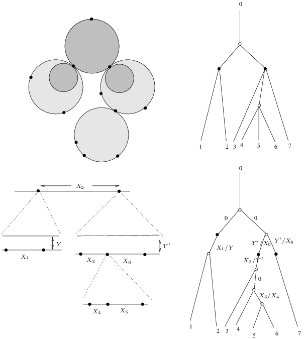
We claim that the map is defined for all with all the ratios landing in , and with the property that if and only if the combinatorial type of has the edge . To see this, recall that if , its combinatorial type must be obtained from by contracting a subset of edges (that is, ). In particular, every edge in corresponds to a unique edge in . Hence, if connects a vertex with a vertex above it, then in either if is contracted, or the edge remains. If in , it implies that the disk component of on which is also the disk component on which , hence and and the ratio . If the edge remains in , it means that with respect to the markings on the disk component where , we have and so
Now if connects vertex with a colored vertex above it, then in either becomes a colored vertex, or is an edge. In the first case, it implies that the unique component where is a quilted component, so parametrizing the component such that the inner circle is a line of height , and . In the second case, the unique component where is unquilted and corresponds to having the line at height , so . The case of a colored vertex below is similar. This completes the construction of .


Definition 6.1.
Let be a colored tree. A labelling is balanced if it satisfies the following condition: denote by the set of vertices on the root side of the colored vertices, that is, connected to the root by a path not crossing a colored vertex. For each vertex and any colored vertex connected by a path of edges not crossing the root, let denote the product of the values of along the unique path of edges from to . Then is balanced if is independent of the choice of colored vertex . Let denote the set of balanced labellings:
We denote by the subset of non-zero labellings.
Proposition 6.2.
Let be a maximal colored tree. Then is a homeomorphism from onto , mapping onto .
Thus in particular the simple-ratios and cross-ratios define the same topology on .
Proof.
It follows from the definition that takes values in balanced labellings, with products where is the top vertex. The construction of also makes it clear how to construct a pointed nodal quilted disk from a balanced labeling of , showing that is onto . To make the relationship between the coordinates in the balanced labeling and the cross-ratio coordinates in a chart for explicit, let be the cross-ratios in a chart covering . Without loss of generality, assume that all chart cross-ratios of the form are either of the form , or , so that on they take values in , and such that for , implies that the combinatorial type of has the edge . Let denote the simple ratios in a balanced labelling of . We claim that for every edge , where is a smooth function on the interior of which is continuous up to the boundary, and on . In particular, . First we prove it for the cross-ratios in the chart. By symmetry it suffices to consider the edge pictured in Figure 10, where an edge joins vertices and , with above , so , and a chart cross-ratio for is .


Parametrizing so that ,
The ratios in the bracketed function are products of ratios labeling edges below and , and the presence of the 1’s means that bracketed function is smooth and never zero for all positive non-zero ratios and continuous as the labels in the chart go to 0, so if and only if . Now we prove it for a cross-ratio in the chart. Parametrizing so that and using to denote the height of the line with respect to this parametrization, consider an edge such as the one pictured in Figure 10, where the cross-ratio labelling in a cross-ratio chart is , and the simple ratio . Then
where the ratios appearing in the big bracket are products of simple ratios labelling edges below . The function is smooth and never for all positive non-zero ratios and it is continuous as ratios . Moreover if and only if . The case of a colored vertex above a regular vertex is very similar so we omit it. This proves that the transition from a simple ratio chart to a cross ratios chart is a smooth change of coordinates on . ∎
One sees from this description that is not a manifold-with-corners. We say that a point is a singularity if is not CW-isomorphic to a manifold with corners near .
Example 6.3.
The first singular point occurs for . The expression is adjacent to the expressions , , , and hence there are four edges coming out of the corresponding vertex. On the other hand, the dimension of is , see Figure 11. Thus cannot be a manifold with corners (and therefore, not a simplicial polytope.)


.
Lemma 6.4.
Any morphism of trees induces a morphism of balanced labellings .
Proof.
Let be a morphism of trees. Given a balanced labelling we obtain a balanced labelling by setting where the product is over edges above that are collapsed under . One sees easily that the resulting labelling of is balanced. ∎
Corollary 6.5.
Let be a colored tree. There exists a CW-isomorphism of onto a neighborhood of in .
Proof.
Let be a maximal tree such that there exists a morphism of trees . For each vertex , let be the subtree whose vertices map to . Given a labelling , we obtain by restriction labellings for each , and from Lemma 6.4 a labelling . Thus we obtain a map
It is straightforward to verify that this map induces an isomorphism of onto The former is the image of under . Since each tree is maximal, Proposition 6.2 gives an isomorphism of onto ∎
For later use, we describe subsets of the edges whose labels determine all others.
Definition 6.6.
Let be a maximal colored tree. Let be an interior edge of that is incident to a pair of trivalent vertices. Contraction of produces a 4-valent vertex, and we say that the tree obtained by a flop of is that which corresponds to the alternative resolution of the 4-valent vertex. A fusion move through an interior vertex is one by which two colored vertices immediately below become a single colored vertex immediately above ; we call the reverse move a splitting move. We say that two maximal colored trees and differ by a basic move if they differ by a single flop, fusion, or splitting move.

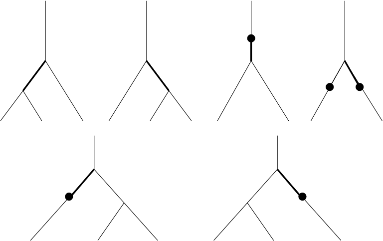
Any maximal colored tree can be obtained from a fixed maximal colored tree by a sequence of basic moves. Let be a maximal colored tree. The simple ratios chart covering the open set assigns a simple ratio coordinate to each interior edge of ; however, on a given chart, some of those ratios may be functions of other ratios in the chart. There are six possibilities for an interior edge of , pictured in Figure 13. Note that the edges in the top four cases have a basic move associated to them, but not the two lower cases.
Lemma 6.7.
All simple ratios in are determined by the simple ratios labeling edges which have an associated basic move.
Proof.
The simple ratios for the other edges are redundant: if an edge doesn’t have an associated basic move, it must be one of the lower two types in Figure 13. Let be the vertex directly above . Observe that there must exist a path from to another colored vertex below it, such that every edge in the path is one of the top four types in Figure 13. Thus the simple ratios labeling the edges in that path appear in the reduced chart, and the relations imply that the product of the simple ratios in that path is equal to the simple ratio labeling . ∎
Definition 6.8.
A reduced simple ratio chart is given by restricting to the edges that have an associated basic move; we call these edges reduced chart edges.
Example 6.9.
In the example of Figure 9, the reduced simple ratio chart consists of . The simple ratio is redundant.
7. Colored metric ribbon trees
The multiplihedra have another geometric realization as colored metric ribbon trees. Colored trees were introduced in Boardman-Vogt [2], although their construction does not have the relations described below.
Definition 7.1.
A colored rooted metric ribbon tree is a colored rooted ribbon tree with a metric such that the sum of the edge lengths in any non-self-crossing path from a colored vertex back to the root is independent of . A colored rooted metric ribbon tree is stable if each colored resp. non-colored vertex has valency at least resp. .
Example 7.2.
For the tree in Figure 14, an edge length map is subject to the relations

For each stable colored tree , we denote by the set of all maps colored metric trees with underlying colored tree and by the union
We define a topology on as follows. Assume that a sequence of metric trees converges for each interior edge to a non-negative real number. In other words, for every . We say that the corresponding colored metric trees converge to if
- (a)
is the tree obtained from by collapsing edges for which . This defines a surjective morphism of colored rooted ribbon trees, .
- (b)
- (c)
, if this limit is non-zero.
Proposition 7.3.
is a polyhedral cone in , where .
Proof.
There is an action on , given by , so it is clearly a cone. The dimension follows from the fact that there are variables and relations. The polyhedral structure can be seen by writing variables as linear combinations of independent variables. Then the condition that all means that is an intersection of half-spaces. ∎
Example 7.4.
In the example of Figure 14, , and . We can choose independent variables to be , and express the remaining variables as Thus the space of admissible edge lengths is parametrized by points in the polyhedral cone that is the intersection of (for the independent variables being non-negative) with the half-spaces and .
Exponentiating the labellings of the edges gives a map
Since , the image of a cone is identified directly with the subset of consisting of balanced labellings with for every .
Example 7.5.
Consider the case , where we have fixed the parametrization of the elements of so that the interior circle is identified with a line of height in half-space. Let and . The images of subdivide into 6 regions, see Figure 15, each of which corresponds to a cone in via the homeomorphism .

There is a natural compactification of by allowing edges to have length . The map extends to the compactifications by taking limits in appropriate charts.
Theorem 7.6.
The map is a homeomorphism, with the property that for any combinatorial type , intersects in a single point.
This is the colored analog of Theorem 2.8.
Proof.
As , the identification implies . Thus the image of a compactified cone is identified with the subset of consisting of balanced labellings with for every . ∎
8. Toric varieties and moment polytopes.
In this section we show
Theorem 8.1.
is homeomorphic to the non-negative part of an embedded toric variety in , where is the number of maximal colored trees with leaves.
In particular, is isomorphic as a -complex to a convex polytope; this reproduces the result of Forcey [3]. Using this we prove the main Theorem 1.1. First we define the toric variety . Recall from Section 6 that a point in can be identified with a projective coordinate by parametrizing such that , and setting and to be the height of the line. Let be a maximal colored tree. Adapting the algorithm of Forcey in [3], we associate a weight vector to the tree as follows. A pair of adjacent leaves in , say and , determines a unique vertex in , which we label . Let be the number of leaves on the left side of , and let be the number of leaves on the right side of . Let
Set
Example 8.2.
The tree in Figure 16 has weight vector , and monomial .

Fix some ordering of the maximal colored trees with leaves, . The projective toric variety is the closure of the image of the embedding
| (5) |
The entries in the weight vectors always sum to , so the map is well-defined on the homogeneous coordinates.
Lemma 8.3.
Suppose that two maximal colored trees and differ by a single basic move involving an edge . Let denote the simple ratio labeling the edge in the chart determined by . Then
for an integer . In general, for two maximal trees and ,
for some edges of and positive integers .
Proof.
First let us consider the case of a single flop. Without loss of generality consider the situation in Figure 17. Say is on the left, and is on the right, and the affected edges are in bold.

The weight vectors and are the same in all entries except entries and , where
Therefore,
and observe that is the ratio labeling that edge of , and .
For the other kinds of basic move it suffices to consider fusion, in which a pair of colored vertices are below in , and above in . The weight vectors of and are identical in all entries except for the -th entry, which corresponds to the exponent of , and the -th entry, which corresponds to the exponent of :
Therefore
where is the ratio labeling the two edges below of , and .
The vertices are partially ordered by their positions in the tree; the effect of basic moves on the partial ordering are individual changes , or , between adjacent vertices. In general, every maximal tree is obtained from a fixed tree by a sequence of independent basic moves – by independent we just mean that each one involves a different pair of vertices. We prove the general case by induction on the number of independent basic moves needed to get from a fixed maximal tree , to any other maximal tree . Having proved the base case, now consider a tree obtained after a sequence of flops. Write for a tree which is independent moves away from and one move away from . Suppose that the the final move between and is described by the . By the inductive hypothesis and the base step,
for some positive integers and , and some edges of . Since none of the previous flops involved the pair and , the partial order in the original tree must have also had , although they were possibly not adjacent in . In any case, the ratio is a product of the ratios in the chart labeling the edges from to . The case where the final move is one of is similarly straightforward. This completes the inductive step. ∎
Proof of Theorem 8.1.
We use Lemma 8.3 to identify the simple ratios in a reduced chart for each maximal colored tree , with the non-negative part of the affine slice . Consider . The affine piece consists of all points
where the entries may be 0. Now let be the simple ratio coordinates in a reduced chart for the open set (Definition 6.8). By construction, the edges of have associated basic moves. Thus they determine a set of maximal colored trees, where each is obtained from by the basic move associated to the edge . Without loss of generality, assume that the maximal trees are respectively . By Lemma 8.3, we identify the non-negative part of with the chart by the map
where are positive integers depending on the combinatorics of , and the entries labeled are higher products of . This map is well-defined, one-to-one and onto for and which are all in the non-negative range . ∎
Corollary 8.4.
is -isomorphic to the convex hull of the weight vectors in , and thus -isomorphic to a -dimensional polytope.
Proof.
Proof of Theorem 1.1.
By induction on : The one-dimensional spaces and are all compact and connected, and so -isomorphic. It suffices, therefore, to show that is the cone on its boundary. This is true since it is homeomorphic to a convex polytope. ∎
9. Stable weighted disks
Fukaya, Oh, Ohta, and Ono [4] introduced another geometric realization of the multiplihedron, although the CW-structure is slightly different. A weighted stable -marked disk consists of
- (a)
a stable nodal disk
- (b)
for each component of , a weight
with the following property: if is further away from from the root marking then . An isomorphism of rooted stable disks is an isomorphism of stable disks intertwining with the weights. Let denote the moduli space of stable weighted marked disks, equipped with the natural extension of the Gromov topology in which a sequence converges to if Gromov converges to and the weights on the limit curve are pulled back from those on via the morphism of trees appearing in the limit.
For example, is an interval; is a hexagon consisting of a square and two triangles, joined along two edges, see Figure 18. Each triangle is defined by the inequality . The moduli space has cells of dimension on the boundary ( projecting onto -cell of , projecting onto -cells of , and projecting onto vertices of .) On the other hand, the multiplihedron has cells of dimension on the boundary, see Figure 11.
10. Stable scaled affine lines.
In this section we re-interpret the moduli space of quilted disks as a moduli space of stable scaled lines. This construction has the advantage that it works for any field. Working over gives a moduli space introduced Ziltener’s study [14] of gauged pseudoholomorphic maps from the complex plane; we show it is a projective variety with toric singularities.
Definition 10.1.
Let be a field. A scaled marked line is a datum , where is an affine line over , are distinct points, and is a translationally invariant area form. An isomorphism of scaled marked lines is an isomorphism that intertwines the area forms and markings. A scaled line is stable if the automorphism group is finite, that is, has at least one marking. Denote by the corresponding moduli space of stable, scaled marked lines.
In the case , has as a component (given by requiring that the markings appear in order) the moduli space of the previous section, through identifying with , where is a line of height . has a natural compactification, obtained by allowing the points to come together and the volume form to scale. For any nodal curve with markings , and component of , we write for the special point in that is either the marking , or the node closest to .
Definition 10.2.
A (genus zero) nodal scaled marked line is a datum , where is a (genus zero) projective nodal curve, is a collection of markings disjoint from the nodes, and for each component of , the affine line is equipped with a (possibly zero or infinite) translationally invariant volume form . We call a volume form degenerate if it is zero or infinite. An automorphism of a stable nodal scaled curve is an automorphism of the nodal curve preserving the volume forms and the markings. A nodal scaled marked curve is stable if it has finite automorphism group, or equivalently, if each component with non-degenerate (resp. degenerate) volume form has at least two (resp. three) special points.
The affine structure on is unique up to dilation, so that is well-defined. The combinatorial type of a nodal scaled marked affine line is a rooted colored tree: Vertices represent components of the nodal curve, edges represent nodes, labeled semi-infinite edges represent the markings, with the root always labelled by . Every path from a leaf back to the root must pass through exactly one colored vertex.
Now we specialize to the case . contains as a subspace those scaled marked curves such that all markings lie on the projective real line, ; these are naturally identified with marked disks. More accurately, admits an antiholomorphic involution induced by the antiholomorphic involution of . The involution extends to an antiholomorphic involution of . The multiplihedron can be identified with the subset of the fixed point set such that the points are in the required order.
We introduce coordinates on in the same way as we did for . Define two types of coordinates, of the form where are distinct indices in , and of the form , where are distinct indices in . The are defined as before, and the are defined as follows: given a representative ,
The coordinates extend to the compactification . For the coordinates , we evaluate the cross-ratio at a component in the bubble tree for which at least three of and are distinct, normalizing by
| (6) |
For the coordinates , we evaluate them at the unique component at which and are distinct, normalizing by
The same arguments as in the real case show that the product of forgetful morphisms defines an embedding
The coordinates and also satisfy recursion relations
Let denote the closure of the algebraic variety defined by the two types of cross ratio coordinate and the relations (10).
Theorem 10.3.
The map is a bijection.
The proof of the bijection is an extension of the corresponding result for genus zero stable nodal -pointed curves, . In this case the cross-ratios satisfy (10). Let denote the closure of the algebraic variety defined by the cross-ratio coordinates and the relation (10). The image of the canonical embedding with cross-ratios is contained in , the map is a bijection [9, Theorem D.4.5].
Proof of Theorem 10.3.
First we show that is injective. Given a nodal stable scaled marked line , by construction the combinatorial type uniquely determines which cross-ratios are or , and which cross-ratios are and . In addition, the isomorphism class of each component of is determined by the cross-ratios with values in and with values in , so the map is injective. To show that is surjective, let . By the result for stable curves [9, D.4.5], there is a unique stable, nodal -marked genus zero curve of combinatorial type given by a rooted tree (the root corresponds to the marking ), which realizes the cross-ratios of the form .
Lemma 10.4.
Let , and suppose that for some , are distinct at .
- (a)
If , then for every vertex in a path from to the root (including itself), for every distinct triple .
- (b)
If , then for every vertex in a path from away from the root (including itself), for every distinct triple .
- (c)
If , then
- (i)
for every other distinct triple on , ;
- (ii)
for every vertex adjacent to towards the root, and every distinct triple , ;
- (iii)
for every vertex adjacent to away from the root, and every distinct triple , .
- (i)
Proof.
(a) First, we show that for every such that are distinct. Without loss of generality suppose that is distinct from and . Then and so by (10), . Now without loss of generality suppose that is distinct from and . Then so by (10) . Now consider the vertex that is immediately adjacent to in the direction of the root. Without loss of generality, suppose that is distinct from . The combinatorics of at and imply that , hence by (10), . Applying the first argument that for all with distinct. The result holds by remaining vertices in the path from by induction. (b) First, we show that for every such that are distinct. Without loss of generality suppose that is distinct from and . Then , hence by (10) . Now without loss of generality suppose that is distinct from and . Then hence by (10) . Now consider a vertex that is immediately adjacent to away from the root. It is now enough to show that for some such that and are distinct. Pick and such that are distinct (hence by the previous argument ), and such that is adjacent to through a node that identifies with . Now let be distinct from and . Then , so by (10), .
(c) Proof of (i): If is distinct from and , then so hence . Repeating this argument implies that for any and such that are distinct. Proof of (ii): In light of (a) and the proof of (c)(i), it is enough to prove that for any such that and are distinct, then . Note that since is closer to the root than , . Hence, , and by (10), . Proof of (iii): In light of (b) and (c)(i), it is enough to prove the following case: if is incident to in such a way that is distinct from and , then . In this case, , so (10) implies .
∎
By Lemma 10.4, the vertices of the tree can be partitioned into subsets for which the cross-ratios defined on them are 0, , or finite non-zero. Let
If is empty, turn the marked point into a nodal point and attach it to the nodal point of a scaled curve . If is non-empty, by Lemma 10.4 it must be a connected sub-tree which includes the component containing the root . If a marked point , is on a component labeled by , turn the marked point into a nodal point and attach it to the nodal point of a scaled curve . If then by Lemma 10.4 it is attached by a node to . Suppose that and are distinct and . Identify this sphere component and its markings with a stable marked curve with the same markings, and a volume form determined by parametrizing and putting . Finally, suppose that is connected by a nodal point to a nodal point of . Then insert a stable marked curve such that the node identifications are with , and with .
At the end of this process one obtains a stable nodal, marked scaled curve in , whose combinatorial type is a colored tree refining the tree , and whose image under the cross-ratio embedding is the same as the original point . ∎
Given the combinatorial type of a stable scaled curve, one can choose a local chart of cross-ratios according to the same prescription as given in the real case.
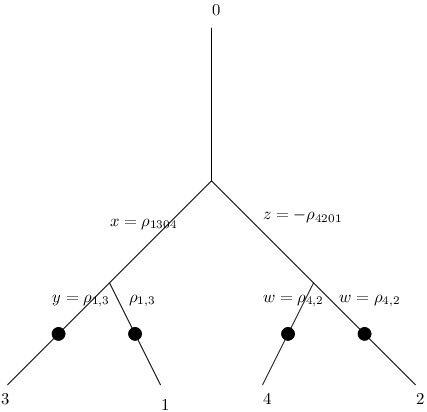
The subset of points with non-zero labels is the kernel of the homomorphism given by taking the product of labels from the given vertex to the colored vertex above it, and is therefore an algebraic torus. The torus acts on by multiplication with a dense orbit. Choose a planar structure on . Let
denote the map given by the simple ratios in Definition (4) (now allowed to be complex). After re-labelling it suffices to consider the case that the ordering is the standard ordering. We denote by the Zariski open subset of defined by the equations , for .
Theorem 10.5.
is an isomorphism of onto .
Proof.
Let be a maximal colored tree and consider the map given by the simple ratios. The same argument as in the real case shows that any is in the image of some quilted disk unless at some stage the reconstruction procedure assigns the same position to two markings in different branches; in this case we have . The set of exceptional points in is an affine subvariety of disjoint from hence the Theorem. ∎
Corollary 10.6.
Let be a colored tree. There exists an isomorphism of a Zariski open neighborhood of in with a Zariski open neighborhood of in . Thus is a projective variety with at most toric singularities.
The proof is similar to the real case in Corollary 6.5 and left to the reader. This completes the proof of Theorem 1.2 in the introduction.
References
- [2] J. M. Boardman and R. M. Vogt. Homotopy invariant algebraic structures on topological spaces. Springer-Verlag, Berlin, 1973. Lecture Notes in Mathematics, Vol. 347.
- [3] Stefan Forcey. Convex hull realizations of the multiplihedra. arXiv:math.AT/0706.3226.
- [4] K. Fukaya, Y.-G Oh, H. Ohta and K.Ono. Lagrangian intersection Floer theory: anomaly and obstruction. Book in preparation.
- [5] Kenji Fukaya and Yong-Geun Oh. Zero-loop open strings in the cotangent bundle and Morse homotopy. Asian J. Math., 1(1):96–180, 1997.
- [6] William Fulton. Introduction to toric varieties, volume 131 of Annals of Mathematics Studies. Princeton University Press, Princeton, NJ, 1993. , The William H. Roever Lectures in Geometry.
- [7] Norio Iwase and Mamoru Mimura. Higher homotopy associativity. In Algebraic topology (Arcata, CA, 1986), volume 1370 of Lecture Notes in Math., pages 193–220. Springer, Berlin, 1989.
- [8] M. Kontsevich and Yu. Manin. Gromov-Witten classes, quantum cohomology, and enumerative geometry [ MR1291244 (95i:14049)]. In Mirror symmetry, II, volume 1 of AMS/IP Stud. Adv. Math., pages 607–653. Amer. Math. Soc., Providence, RI, 1997.
- [9] Dusa McDuff and Dietmar Salamon. -holomorphic curves and symplectic topology, volume 52 of American Math. Soc. Colloq. Pub.. American Mathematical Society, Providence, RI, 2004.
- [10] Khoa Nguyen and Chris Woodward. Morphisms of cohomological field theories. 2008 preprint.
- [11] Frank Sottile. Toric ideals, real toric varieties, and the moment map. In Topics in algebraic geometry and geometric modeling, volume 334 of Contemp. Math., pages 225–240. Amer. Math. Soc., Providence, RI, 2003.
- [12] James Stasheff. -spaces from a homotopy point of view. Lecture Notes in Mathematics, Vol. 161. Springer-Verlag, Berlin, 1970.
- [13] James Dillon Stasheff. Homotopy associativity of -spaces. I, II. Trans. Amer. Math. Soc. 108 (1963), 275-292; ibid., 108:293–312, 1963.
- [14] F. Ziltener. Symplectic vortices on the complex plane and quantum cohomology. PhD thesis, Zurich, 2006.