跳到论文正文
W Papers独立论文阅读器 arXiv:0802.2075 论文正文 计算阅读时间 · 0%
引用这篇论文根据当前论文元数据生成,正式投稿前建议核对。


License: arXiv.org perpetual non-exclusive license
arXiv:0802.2075v1 [hep-ph] 14 Feb 2008

Combined effects of strong and electroweak FCNC effective operators in top quark physics at the LHC

P.M. Ferreira1,2 , R.B. Guedes2  and R. Santos2,3 Note: ferreira@cii.fc.ul.pt Note: renato@cii.fc.ul.pt Note: rsantos@cii.fc.ul.pt Affiliation: 1 Instituto Superior de Engenharia de Lisboa, Rua Conselheiro Emídio Navarro, 1, 1959-007 Lisboa, Portugal
2 Centro de Física Teórica e Computacional, Faculdade de Ciências, Universidade de Lisboa, Avenida Professor Gama Pinto, 2, 1649-003 Lisboa, Portugal
3 Department of Physics, Royal Holloway, University of London, Egham, Surrey TW20 0EX United Kingdom
February, 2008
Abstract

We study the combined effects of both strong and electroweak dimension six effective operators on flavour changing top quark physics at the LHC. Analytic expressions for the cross sections and decay widths of several flavour changing processes will be presented, as well as an analysis of the feasibility of their observation at the LHC.

pacs
PACS number(s): 14.65.Ha, 12.15.Mm, 12.60.-i

I Introduction

The LHC will soon begin operating, and the number of top quarks produced in it is of the order of millions per year. Such large statistics will enable precision studies in top quark physics - this being the least well-know elementary particle discovered so far. The study of flavour changing neutral current (FCNC) interactions of the top quark is of particular interest. In fact, the FCNC decays of the top - decays to a quark of a different flavour and a gauge boson, or a Higgs scalar - have branching ratios which can vary immensely from model to model - from the extremely small values expected within the Standard Model (SM) to magnitudes possibly measurable at the LHC in certain SM extensions.

The use of anomalous couplings to study possible new top physics at the LHC and Tevatron has been the subject of many works [1]. In a recent series of papers [2, 3, 4] we considered FCNC interactions associated with the strong interaction - decays of the type t→u​gt\rightarrow u\,g or t→c​gt\rightarrow c\,g - describing them using the most general dimension six FCNC lagrangian emerging from the effective operator formalism [5]. The FCNC vertices originating from that lagrangian also had substantial contributions to processes of production of the top quark, such as associated production of a single top quark alongside a jet, a Higgs boson - or an electroweak gauge boson. The study of refs. [2, 3, 4] concluded that, for large values of B​R​(t→q​g)BR(t\rightarrow q\,g), with q=u,cq=u,c, these processes of single top production might be observable at the LHC.

What about the possibility of FCNC associated with the electroweak sector - FCNC interactions leading to decays of the form t→q​γt\rightarrow q\,\gamma or t→q​Zt\rightarrow q\,Z ? In some extensions of the SM these branching ratios can be as large as, if not larger, those of the strong FCNC interactions involving gluons. In the current paper we extend the analysis of our previous works and consider the most general dimension six FCNC lagrangian in the effective operator formalism which leads to t→q​γt\rightarrow q\,\gamma and t→q​Zt\rightarrow q\,Z decays. We will study the effects of these new electroweak FCNC interactions in the decays of the top quark and its expected production at the LHC. We will study in detail processes - such as t+γt\,+\,\gamma and t+Zt\,+\,Z production - for which both strong and electroweak FCNC interactions contribute. The automatic gauge invariance of the effective operator formalism will allow us to detect correlations between several FCNC observables. The FCNC processes p​p→t​Zpp\rightarrow t\,Z and p​p→t​γpp\rightarrow t\,\gamma were studied in great detail for the Tevatron in [6] and for the LHC in [7]. We will draw heavily on the results of those references, all the while emphasising the differences in our approaches: (a) our chief aim is to provide the scientific community with analytical expressions anyone can use to built event generators and perform detailed studies of FCNC at the LHC; (b) we show all results in terms of measurable quantities, such as branching ratios, and not in terms of the values of the anomalous couplings; and (c), our formalism leads us to to write FCNC vertices different from those of refs. [6, 7], and to uncover connections between several FCNC quantities.

This paper is organised as follows: in section II we review the effective operator formalism and introduce our FCNC operators, explaining what physical criteria were behind their choice. We also present the Feynman rules for the new anomalous top quark interactions which will be the base of all the work that follows. In section III we use those same Feynman rules to compute and analyse the branching ratios of the top quark FCNC decays, with particular emphasis on the relationship between B​r​(t→q​γ)Br(t\,\rightarrow\,q\,\gamma) and B​r​(t→q​Z)Br(t\,\rightarrow\,q\,Z). In the following two sections we study the cross section for production, at the LHC, of a single top and a photon or a ZZ boson, with all FCNC interactions - both strong and electroweak - included. We also investigate whether it would be possible to conclude, from the data, whether any FCNC phenomena observed would have at its root the strong or the electroweak sectors. Finally, in section V we present a general discussion of the results and some conclusions.

II Flavour changing effective operators

The effective operator formalism of Buchmüller and Wyler [5] is based on the assumption that the Standard Model of particle physics is the low energy limit of a more general theory. Such theory would be valid at very high energies but, at a lower energy scale Λ\Lambda, we would only perceive its effects through a set of effective operators of dimensions higher than four. Those operators would obey the gauge symmetries of the SM, and be suppressed by powers of Λ\Lambda. This allows us to write this effective lagrangian as a series, such that

ℒ=ℒS​M+1Λ​ℒ(5)+1Λ2​ℒ(6)+O⁡(1Λ3),{\cal L}\;\;=\;\;{\cal L}^{SM}\;+\;\frac{1}{\Lambda}\,{\cal L}^{(5)}\;+\;\frac{1}{\Lambda^{2}}\,{\cal L}^{(6)}\;+\;O\,\left(\frac{1}{\Lambda^{3}}\right)\;\;\;, (1)

where ℒS​M{\cal L}^{SM} is the SM lagrangian and ℒ(5){\cal L}^{(5)} and ℒ(6){\cal L}^{(6)} contain all the dimension five and six operators which, like ℒS​M{\cal L}^{SM}, are invariant under the gauge symmetries of the SM. The list of dimension six operators is quite vast [5]. This formalism allows us to parameterize new physics, beyond that of the SM, in a model-independent manner.

In this work we are interested in effective operators of dimension six that contribute to flavour-changing interactions of the top quark in the weak sector. The ℒ(5){\cal L}^{(5)} terms break baryon and lepton number conservation, and therefore we do not consider them in this analysis. This work follows refs. [2, 3, 4], where we considered FCNC top effective operators which affect the strong sector. Namely, operators which, amongst other things, contribute to FCNC decays of the form t→u​gt\,\rightarrow\,u\,g or t→c​gt\,\rightarrow\,c\,g. The operators we considered were expressed as

𝒪t​G\displaystyle{\cal O}_{tG} =i​αi​tSΛ2​(u¯Ri​λa​γμ​Dν​tR)​Ga​μ​ν,𝒪t​G​ϕ=βi​tSΛ2​(q¯Li​λa​σμ​ν​tR)​ϕ~​Gμ​νa,\displaystyle=i\frac{\alpha^{S}_{it}}{\Lambda^{2}}\,\left(\bar{u}^{i}_{R}\,\lambda^{a}\,\gamma_{\mu}D_{\nu}t_{R}\right)\,G^{a\mu\nu}\;\;\;,\;\;\;{\cal O}_{tG\phi}=\frac{\beta^{S}_{it}}{\Lambda^{2}}\,\left(\bar{q}^{i}_{L}\,\,\lambda^{a}\,\sigma^{\mu\nu}\,t_{R}\right)\,\tilde{\phi}\,G^{a}_{\mu\nu}\;\;\;, (2)

where the coefficients αi​tS\alpha^{S}_{it} and βi​tS\beta^{S}_{it} are complex dimensionless couplings. The fields uRiu^{i}_{R} and qLiq^{i}_{L} represent the right-handed up-type quark and left-handed quark doublet of the first and second generation - this way FCNC occurs. Gμ​νaG^{a}_{\mu\nu} is the gluonic field tensor. There are also operators, with couplings αt​iS\alpha^{S}_{ti} and βt​iS\beta^{S}_{ti}, where the positions of the top and uîu^{î}, qiq^{i} spinors are exchanged in the expressions above. Also, the hermitian conjugates of all of these operators are obviously included in the lagrangian. These operators contribute to FCNC vertices of the form g​t​ui¯g\,t\,\bar{u_{i}} (with ui=u,cu_{i}\,=\,u\,,\,c). The operators with αS\alpha^{S} couplings, due to their gauge structure (namely, the covariant derivative acting on a quark spinor), also contribute to quartic vertices of the form g​g​t​ui¯g\,g\,t\,\bar{u_{i}}, g​γ​t​ui¯g\,\gamma\,t\,\bar{u_{i}} and g​Z​t​ui¯g\,Z\,t\,\bar{u_{i}}.

Our criteria in choosing these operators were that they contributed only to FCNC top physics, not affecting low energy physics. In that sense, operators that contributed to top quark phenomenology but which also affected bottom quark physics (in the notation of ref. [5], operators 𝒪q​G{\cal O}_{qG}) were not considered. Recently, a study based on constraints from B physics [8] using the predictions for the LHC [9, 10, 11], has showed that, in fact, some of the constraints on dimension 6 operators stemming from low energy physics are already stronger than some of the predictions for the LHC. This is true for the operators denoted in [8] by L​LLL, which are the ones built with two S​U​(2)SU(2) doublets that we had left out in our previous work. Obviously the gauge structure is felt more strongly in the left-left (LL) type of operators than in the right-right type. Hence, they concluded that the LL operators will not be probed at the LHC because they are already constrained beyond the expected bounds obtained for a luminosity of 100 f​b−1fb^{-1}. Limits on LR and RL operators are close to those experimental bounds and RR operators are the ones that will definitely be probed at the LHC. Moreover, since more results will come from the B factories and the Tevatron, the constraints will be even stronger by the time the LHC starts to analyse data. Therefore our criteria in the choice of operators is well founded, and we will also not consider LL operators in the electroweak sector.

II.1 Effective operators contributing to electroweak FCNC top decays

According to our criteria of leaving low-energy particle physics unchanged, we will now consider all possible dimension six effective operators which contribute to top decays of the form t→ui​γt\,\rightarrow\,u_{i}\,\gamma and t→ui​Zt\,\rightarrow\,u_{i}\,Z. First we have the operators analogous to those of eq. (2) in the electroweak sector, to wit,

𝒪t​B=i​αi​tBΛ2​(u¯Ri​γμ​Dν​tR)​Bμ​ν,\displaystyle{\cal O}_{tB}=i\frac{\alpha^{B}_{it}}{\Lambda^{2}}\,\left(\bar{u}^{i}_{R}\,\,\gamma_{\mu}D_{\nu}t_{R}\right)\,B^{\mu\nu}\;\;\;, 𝒪t​B​ϕ=βi​tBΛ2​(q¯Li​σμ​ν​tR)​ϕ~​Bμ​ν,\displaystyle\;\;\;{\cal O}_{tB\phi}=\;\;\frac{\beta^{B}_{it}}{\Lambda^{2}}\,\left(\bar{q}^{i}_{L}\,\sigma^{\mu\nu}\,t_{R}\right)\,\tilde{\phi}\,B_{\mu\nu}\;\;\;,
𝒪t​W​ϕ=βi​tWΛ2​(q¯Li​τI​σμ​ν​tR)​ϕ~​Wμ​νI,\displaystyle{\cal O}_{tW\phi}=\frac{\beta^{W}_{it}}{\Lambda^{2}}\,\left(\bar{q}^{i}_{L}\,\,\tau_{I}\,\sigma^{\mu\nu}\,t_{R}\right)\,\tilde{\phi}\,W^{I}_{\mu\nu}\;\;\;, (3)

where αt​iB\alpha^{B}_{ti}, βt​iB\beta^{B}_{ti} and βt​iW\beta^{W}_{ti} are complex dimensionless couplings, and Bμ​νB^{\mu\nu} and Wμ​νIW^{I}_{\mu\nu} are the U​(1)YU(1)_{Y} and S​U​(2)LSU(2)_{L} field tensors, respectively. As before, we also consider the operators with exchanged quark spinors, corresponding to couplings αt​iB\alpha^{B}_{ti}, βt​iB\beta^{B}_{ti} and βt​iW\beta^{W}_{ti}, and the hermitian conjugates of all of these terms.

The electroweak tensors “contain” both the photon and ZZ boson fields, through the well-known Weinberg rotation. Thus they contribute simultaneously to vertices of the form Z​t¯​uiZ\,\bar{t}\,u_{i} and γ​t¯​ui\gamma\,\bar{t}\,u_{i} when we consider the partial derivative of DμD^{\mu} in the equations (3), or when we replace the Higgs field ϕ\phi by its vev vv in them. We will isolate the contributions to FCNC photon and ZZ interactions in these operators defining new effective couplings {αγ,βγ}\{\alpha^{\gamma}\,,\,\beta^{\gamma}\} and {αZ,βZ}\{\alpha^{Z}\,,\,\beta^{Z}\}. These are related to the initial couplings via the Weinberg angle θW\theta_{W} by

αγ=cos⁡θW​αB,αZ=−sin⁡θW​αB\alpha^{\gamma}\;=\;\cos\theta_{W}\,\alpha^{B}\qquad\;,\;\qquad\alpha^{Z}\;=\;-\sin\theta_{W}\,\alpha^{B} (4)

and

{βγ=sin⁡θW​βW+cos⁡θW​βBβZ=cos⁡θW​βW−sin⁡θW​βB.\left\{\begin{array}[]{c}\beta^{\gamma}\,=\,\sin\theta_{W}\beta^{W}+\cos\theta_{W}\beta^{B}\\ \beta^{Z}\,=\,\cos\theta_{W}\beta^{W}-\sin\theta_{W}\beta^{B}\\ \end{array}\right.. (5)

As we will see, these Weinberg rotations will introduce a certain correlation between FCNC processes involving the photon or the ZZ.

Because the Higgs field is electrically neutral but has weak interactions, there are more effective operators which will only contribute to new ZZ FCNC interactions. They are analogous to operators considered in [12] for study of FCNC in the leptonic sector and are given by

𝒪Dt\displaystyle{\cal O}_{D_{t}} =ηi​tΛ2​(q¯Li​Dμ​tR)​Dμ​ϕ~,𝒪D¯t=η¯i​tΛ2​(Dμ​q¯Li​tR)​Dμ​ϕ~\displaystyle=\frac{\eta_{it}}{\Lambda^{2}}\,\left(\bar{q}^{i}_{L}\,D^{\mu}\,t_{R}\right)\,D_{\mu}\tilde{\phi}\,\;\;\;,\;\;\;{\cal O}_{\bar{D}_{t}}=\frac{\bar{\eta}_{it}}{\Lambda^{2}}\,\left(D^{\mu}\bar{q}^{i}_{L}\,\,t_{R}\right)\,D_{\mu}\tilde{\phi} (6)

and

𝒪ϕt=θi​t​(ϕ†​Dμ​ϕ)​(uRi¯​γμ​tR),{\cal O}_{\phi_{t}}\,=\,\theta_{it}\,(\phi^{\dagger}D_{\mu}\phi)\,(\bar{u^{i}_{R}}\gamma^{\mu}t_{R})\;\;\;, (7)

and another operator with coupling θt​i\theta_{ti} with the position of the uiu^{i} and tt spinors exchanged. As before, the coefficients ηi​t\eta_{it}, η¯i​t\bar{\eta}_{it} and θi​t\theta_{it} are complex dimensionless couplings.

II.2 Feynman rules for top FCNC weak interactions

The complete effective lagrangian can now be written as a function of the operators defined in the previous section,

ℒ\displaystyle{\cal L} =i​αi​tBΛ2​(u¯Ri​γμ​Dν​tR)​Bμ​ν+i​αt​iBΛ2​(t¯R​γμ​Dν​uRi)​Bμ​ν\displaystyle=\,i\frac{\alpha^{B}_{it}}{\Lambda^{2}}\,\left(\bar{u}^{i}_{R}\,\,\gamma_{\mu}D_{\nu}t_{R}\right)\,B^{\mu\nu}\;+\;i\frac{\alpha^{B}_{ti}}{\Lambda^{2}}\,\left(\bar{t}_{R}\,\,\gamma_{\mu}D_{\nu}u^{i}_{R}\right)\,B^{\mu\nu}\vskip 8.5359pt
+βi​tWΛ2​(q¯Li​τI​σμ​ν​tR)​ϕ​Wμ​νI+βt​iWΛ2​(t¯L​τI​σμ​ν​uRi)​ϕ~​Wμ​νI\displaystyle\;+\;\frac{\beta^{W}_{it}}{\Lambda^{2}}\,\left(\bar{q}^{i}_{L}\,\,\tau_{I}\,\sigma^{\mu\nu}\,t_{R}\right)\,\phi\,W^{I}_{\mu\nu}\;+\;\frac{\beta^{W}_{ti}}{\Lambda^{2}}\,\left(\bar{t}_{L}\,\,\tau_{I}\,\sigma^{\mu\nu}\,u^{i}_{R}\right)\,\tilde{\phi}\,W^{I}_{\mu\nu}\vskip 8.5359pt
+βi​tBΛ2​(q¯Li​σμ​ν​tR)​ϕ~​Bμ​ν+βt​iBΛ2​(t¯L​σμ​ν​uRi)​ϕ​Bμ​ν\displaystyle\;+\;\frac{\beta^{B}_{it}}{\Lambda^{2}}\,\left(\bar{q}^{i}_{L}\,\sigma^{\mu\nu}\,t_{R}\right)\,\tilde{\phi}\,B_{\mu\nu}\;+\;\frac{\beta^{B}_{ti}}{\Lambda^{2}}\,\left(\bar{t}_{L}\,\sigma^{\mu\nu}\,u^{i}_{R}\right)\,\phi\,B_{\mu\nu}\vskip 8.5359pt
+ηi​tΛ2​(q¯Li​Dμ​tR)​Dμ​ϕ~+η¯i​tΛ2​(Dμ​q¯Li​tR)​Dμ​ϕ~\displaystyle\;+\;\frac{\eta_{it}}{\Lambda^{2}}\,\left(\bar{q}^{i}_{L}\,D^{\mu}\,t_{R}\right)\,D_{\mu}\tilde{\phi}\;+\;\frac{\bar{\eta}_{it}}{\Lambda^{2}}\,\left(D^{\mu}\bar{q}^{i}_{L}\,\,t_{R}\right)\,D_{\mu}\tilde{\phi}\vskip 8.5359pt
+θi​t​(ϕ†​Dμ​ϕ)​(uRi¯​γμ​tR)+θt​i​(ϕ†​Dμ​ϕ)​(tR¯​γμ​uRi)+h.c..\displaystyle\;+\;\theta_{it}\,(\phi^{\dagger}D_{\mu}\phi)\,(\bar{u^{i}_{R}}\gamma^{\mu}t_{R})\;+\;\theta_{ti}\,(\phi^{\dagger}D_{\mu}\phi)\,(\bar{t_{R}}\gamma^{\mu}u^{i}_{R})\;+\;\mbox{h.c.}\;\;\;. (8)

This lagrangian describes new vertices of the form γ​u¯​t\gamma\,\bar{u}\,t, Z​u¯​tZ\,\bar{u}\,t, u¯​t​γ​g\bar{u}\,t\,\gamma\,g and u¯​t​Z​g\bar{u}\,t\,Z\,g (and many others) and their charge conjugate vertices. For simplicity we redefine the η\eta and θ\theta couplings as η→(sin⁡(2​θW)/e)​η\eta\rightarrow(\sin(2\theta_{W})/e)\,\eta and θ→(sin⁡(2​θW)/e)​(θi​t−θt​i∗)\theta\rightarrow(\sin(2\theta_{W})/e)\,(\theta_{it}\,-\,\theta^{*}_{ti}). The Feynman rules for the FCNC triple vertices are shown in figures (1) and (2) 11 1 The Feynman rules for the charge-conjugate vertices are obtained by simple complex conjugation. The exception is the θ\theta term, which due to our definition of the θ\theta coupling in eq. (7), will become −θ∗-\theta^{*} for the vertex Z​u​t¯Z\,u\,\bar{t}..

Refer to caption
Figure 1: Feynman rules for the anomalous vertex γ​t​u¯\gamma\,t\,\bar{u}.
Refer to caption
Figure 2: Feynman rules for the anomalous vertex Z​t​u¯Z\,t\,\bar{u}.

Just like for the anomalous operators in the strong sector, the gauge structure of the terms in eq. (8) gives rise to new quartic vertices. Most of the couplings which contribute to the triple vertices of figs. (1), (2) also contribute to the quartic ones. The Feynman rules for the quartic vertices we will need for this paper are shown in figures (3) and (4). We see

Refer to caption
Figure 3: Feynman rules for the anomalous quartic vertex γ​g​t​u¯\gamma\,g\,t\bar{u}.
Refer to caption
Figure 4: Feynman rules for the anomalous quartic vertex Z​g​t​u¯Z\,g\,t\bar{u}.

that these quartic interactions receive contributions from both the strong and electroweak effective operators. Their presence is mandatory because of gauge invariance and they will be of great importance to obtain several elegant results which we present in section IV.

For comparison, the FCNC lagrangian considered by the authors of ref. [7] consisted in

ℒ\displaystyle\cal{L} =g2cosθW​t¯​γμ​(Xt​qL​γL+Xt​qR​γR)​q​Zμ+g2cosθW​t¯​(kt​q(1)−i​kt​q(2)​γ5)​i​σμ​ν​qνmt​q​Zμ\displaystyle=\;\displaystyle{\frac{g}{2\cos\theta_{W}}}\,\bar{t}\,\gamma_{\mu}\,(X_{tq}^{L}\,\gamma_{L}\,+\,X_{tq}^{R}\,\gamma_{R})\,q\,Z^{\mu}\;+\;\displaystyle{\frac{g}{2\cos\theta_{W}}}\,\bar{t}\,(k_{tq}^{(1)}\,-\,i\,k_{tq}^{(2)}\gamma_{5})\,\displaystyle{\frac{i\sigma_{\mu\nu}q^{\nu}}{m_{t}}}\,q\,Z^{\mu} (9)
+e​t¯​(λt​q(1)−i​λt​q(2)​γ5)​i​σμ​ν​qνmt​q​Aμ+gS​t¯​(ζt​q(1)−i​ζt​q(2)​γ5)​i​σμ​ν​qνmt​Ta​q​Ga​μ+h.c.\displaystyle\;\;\;+\;e\,\bar{t}\,(\lambda_{tq}^{(1)}\,-\,i\,\lambda_{tq}^{(2)}\gamma_{5})\,\displaystyle{\frac{i\sigma_{\mu\nu}q^{\nu}}{m_{t}}}\,q\,A^{\mu}\;+\;g_{S}\,\bar{t}\,(\zeta_{tq}^{(1)}\,-\,i\,\zeta_{tq}^{(2)}\gamma_{5})\,\displaystyle{\frac{i\sigma_{\mu\nu}q^{\nu}}{m_{t}}}\,T^{a}\,q\,G^{a\mu}\;+\;h.c.

Notice that whereas we consider a generic scale Λ\Lambda for new physics, these authors set Λ=mt\Lambda\,=\,m_{t}. Also, it is easy to recognize several of our couplings in the lagrangian above; for instance, we have

g2cosθW​Xt​qR=v2Λ2​θ,\displaystyle\displaystyle{\frac{g}{2\cos\theta_{W}}}\,X_{tq}^{R}\,=\,\displaystyle{\frac{v^{2}}{\Lambda^{2}}}\,\theta\;\;\;, g4cosθWmt​(kt​q(1)−i​kt​q(2))=vΛ2​βq​tZ,\displaystyle\;\;\;\displaystyle{\frac{g}{4\cos\theta_{W}m_{t}}}\,\left(k_{tq}^{(1)}\,-\,i\,k_{tq}^{(2)}\right)\,=\,\displaystyle{\frac{v}{\Lambda^{2}}}\,\beta_{qt}^{Z}\;\;\;,
e2​mt​(λt​q(1)−i​λt​q(2))=vΛ2​βq​tγ,\displaystyle\displaystyle{\frac{\,e}{2\,m_{t}}(\lambda_{tq}^{(1)}\,-\,i\,\lambda_{tq}^{(2)})}\,=\,\displaystyle{\frac{v}{\Lambda^{2}}}\,\beta_{qt}^{\gamma}\;\;\;, gS4​mt​(ξt​q(1)−i​ξt​q(2))=vΛ2​βq​tS.\displaystyle\;\;\;\displaystyle{\frac{g_{S}}{4\,m_{t}}(\xi_{tq}^{(1)}-i\,\xi_{tq}^{(2)})}\,=\,\displaystyle{\frac{v}{\Lambda^{2}}}\,\beta_{qt}^{S}\;\;\;. (10)

Notice that due to our choice of efective operators the couplings of the form βq​t\beta_{qt} and βt​q\beta_{tq}, and others, are treated as independent - meaning, the lagrangian (9) does not contain our couplings βt​q\beta_{tq}. Also, couplings of the form {α,η}\{\alpha\,,\,\eta\} are not present in (9), and the photon and ZZ couplings therein presented are taken to be completely independent, unlike what we considered in our work. Their Xt​qLX_{tq}^{L} coupling hasn’t got an equivalent in our formulation. We could obtain it through a θ\theta-like effective operator, namely,

(ϕ†​Dμ​ϕ)​(qLi¯​γμ​qLj),(\phi^{\dagger}D_{\mu}\phi)\,(\bar{q^{i}_{L}}\gamma^{\mu}q^{j}_{L})\;\;\;, (11)

where one of the quark doublets qiq^{i}, qjq^{j} would contain the top quark. It is easy to see, though, that this operator would have a direct contribution to bottom quark physics, thus violating one of our selection criteria for the anomalous top interactions. One important remark: the authors of ref. [7] do not consider the quartic vertices of figs. (3) and (4) in their calculations of cross sections for t+γt\,+\,\gamma and t+Zt\,+\,Z production. That’s entirely correct, since their analysis does not involve couplings like {α,η}\{\alpha\,,\,\eta\}, the only ones who contribute to those quartic vertices.

III FCNC branching ratios of the top

The top can have FCNC decays in the SM, but not at tree level. As such, the branching ratios of these rare top decays are immensely suppressed in the SM, but can be much larger in extensions of the model. Essentially, the existence of new particles will give new contributions to the top rare decays. The interesting thing is that there can be differences of as much as thirteen orders of magnitude between the SM branching ratios and those in some models, as may be seen in table 1.

Process SM QS 2HDM MSSM R​R\!\!\!\!\!\!\not\hskip 9.24994pt SUSY
t→u​Zt\to uZ 8×10−178\times 10^{-17} 1.1×10−41.1\times 10^{-4} −- 2×10−62\times 10^{-6} 3×10−53\times 10^{-5}
t→u​γt\to u\gamma 3.7×10−163.7\times 10^{-16} 7.5×10−97.5\times 10^{-9} −- 2×10−62\times 10^{-6} 1×10−61\times 10^{-6}
t→u​gt\to ug 3.7×10−143.7\times 10^{-14} 1.5×10−71.5\times 10^{-7} −- 8×10−58\times 10^{-5} 2×10−42\times 10^{-4}
t→c​Zt\to cZ 1×10−141\times 10^{-14} 1.1×10−41.1\times 10^{-4} ∼10−7\sim 10^{-7} 2×10−62\times 10^{-6} 3×10−53\times 10^{-5}
t→c​γt\to c\gamma 4.6×10−144.6\times 10^{-14} 7.5×10−97.5\times 10^{-9} ∼10−6\sim 10^{-6} 2×10−62\times 10^{-6} 1×10−61\times 10^{-6}
t→c​gt\to cg 4.6×10−124.6\times 10^{-12} 1.5×10−71.5\times 10^{-7} ∼10−4\sim 10^{-4} 8×10−58\times 10^{-5} 2×10−42\times 10^{-4}
Table 1: Branching ratios for FCNC decays of the top quark in the SM and several possible extensions: the quark-singlet model (QS), the two-higgs doublet model (2HDM), the minimal supersymmetric model (MSSM) and SUSY with R-parity violation. See ref. [13, 14] for details.

The effective operator formalism allows us to describe, in a model-independent manner, the possible rare decays of the top. In ref. [2] we computed the branching ratios for the FCNC top decays t→q​gt\,\rightarrow\,q\,g, due to the strong sector anomalous operators therein introduced. The decay width for t→u​gt\,\rightarrow\,u\,g is given by

Γ⁡(t→u​g)\displaystyle\Gamma(t\rightarrow ug) =mt312​π​Λ4{mt2|αt​uS+(αu​tS)∗|2+ 16v2(|βt​uS|2+|βu​tS|2)+\displaystyle=\;\frac{m^{3}_{t}}{12\pi\Lambda^{4}}\,\Bigg\{m^{2}_{t}\,\left|\alpha_{tu}^{S}+(\alpha^{S}_{ut})^{*}\right|^{2}\,+\,16\,v^{2}\,\left(\left|\beta_{tu}^{S}\right|^{2}+\left|\beta_{ut}^{S}\right|^{2}\right)\;\;\;+\vskip 8.5359pt
 8vmtIm[(αu​tS+(αt​uS)∗)βt​uS]},\displaystyle\hskip 62.59596pt\,8\,v\,m_{t}\,\mbox{Im}\left[(\alpha_{ut}^{S}+(\alpha^{S}_{tu})^{*})\,\beta_{tu}^{S}\right]\Bigg\}\;\;\;, (12)

with an analogous expression for Γ⁡(t→c​g)\Gamma(t\rightarrow cg), with different couplings. The electroweak sector operators we discussed in the previous section contribute to new FCNC decays, namely, t→u​γt\,\rightarrow\,u\,\gamma (and t→c​γt\,\rightarrow\,c\,\gamma, with a priori different couplings), for which we obtain a width given by the following expression:

Γ⁡(t→u​γ)\displaystyle\Gamma(t\rightarrow u\gamma) =mt364​π​Λ4{mt2|αt​uγ+(αu​tγ)∗|2+ 16v2(|βt​uγ|2+|βu​tγ|2)+\displaystyle=\;\frac{m^{3}_{t}}{64\pi\Lambda^{4}}\,\Bigg\{m^{2}_{t}\,\left|\alpha_{tu}^{\gamma}+(\alpha^{\gamma}_{ut})^{*}\right|^{2}\,+\,16\,v^{2}\,\left(\left|\beta_{tu}^{\gamma}\right|^{2}+\left|\beta_{ut}^{\gamma}\right|^{2}\right)\;\;\;+\vskip 8.5359pt
 8vmtIm[(αu​tγ+(αt​uγ)∗)βt​uγ]}.\displaystyle\hskip 62.59596pt\,8\,v\,m_{t}\,\mbox{Im}\left[(\alpha_{ut}^{\gamma}+(\alpha^{\gamma}_{tu})^{*})\,\beta_{tu}^{\gamma}\right]\Bigg\}\;\;\;. (13)

Notice how similar this result is to eq. (12). We will also have contributions from these operators to t→u​Zt\,\rightarrow\,u\,Z (t→c​Zt\,\rightarrow\,c\,Z), from which we obtain a width given by

Γ⁡(t→u​Z)\displaystyle\Gamma(t\,\rightarrow\,u\,Z) =\displaystyle= (mt2−mZ2)232​mt3​π​Λ4[K1|αu​tZ|2+K2|αt​uZ|2+K3(|βu​tZ|2+|βt​uZ|2)+K4(|ηu​t|2+|η¯u​t|2)\displaystyle\frac{{\left(m_{t}^{2}-m_{Z}^{2}\right)}^{2}}{32\,m_{t}^{3}\,\pi\,\Lambda^{4}}\left[K_{1}\,\left|\alpha^{Z}_{ut}\right|^{2}+K_{2}\,\left|\alpha^{Z}_{tu}\right|^{2}+K_{3}\,(\left|\beta^{Z}_{ut}\right|^{2}+\left|\beta^{Z}_{tu}\right|^{2})+K_{4}\,(\left|\eta_{ut}\right|^{2}+\left|\bar{\eta}_{ut}\right|^{2})\right. (14)
+K5​|θ|2+K6​R​e​[αu​tZ​αt​uZ]+K7​I​m​[αu​tZ​βt​uZ]\displaystyle\qquad+\,K_{5}\,\left|\theta\right|^{2}+K_{6}\,Re\left[\alpha^{Z}_{ut}\,\alpha^{Z}_{tu}\right]+K_{7}\,Im\left[\alpha^{Z}_{ut}\,\beta^{Z}_{tu}\right]
+K8​I​m​[αt​uZ∗​βt​uZ]+K9​R​e​[αu​tZ​θ∗]+K10​R​e​[αt​uZ​θ]\displaystyle\qquad+\,K_{8}\,Im\left[\alpha^{Z^{*}}_{tu}\,\beta^{Z}_{tu}\right]+K_{9}\,Re\left[\alpha^{Z}_{ut}\theta^{*}\right]+K_{10}\,Re\left[\alpha^{Z}_{tu}\theta\right]
+K11Re[βu​tZ(ηu​t−η¯u​t)∗]+K12Im[βt​uZθ]+K13Re[ηu​tη¯u​t∗]],\displaystyle\qquad\left.+\,K_{11}\,Re\left[\beta^{Z}_{ut}(\eta_{ut}-\bar{\eta}_{ut})^{*}\right]+K_{12}\,Im\left[\beta^{Z}_{tu}\,\theta\right]+K_{13}\,Re\left[\eta_{ut}\bar{\eta}_{ut}^{*}\right]\right]\;\;\;,

where the coefficients KiK_{i} are given by

K1\displaystyle K_{1} =\displaystyle= 12​(mt4+4​mt2​mZ2+mZ4)K2=12​(mt2−mZ2)2K3= 4​(2​mt2+mZ2)​v2\displaystyle\frac{1}{2}\,(m_{t}^{4}+4\,m_{t}^{2}\,m_{Z}^{2}+m_{Z}^{4})\qquad K_{2}\,=\,\frac{1}{2}\,(m_{t}^{2}-m_{Z}^{2})^{2}\qquad K_{3}\,=\,4\,(2\,m_{t}^{2}+m_{Z}^{2})\,v^{2}
K4\displaystyle K_{4} =\displaystyle= v24​mZ2​(mt2−mZ2)2K5=v4mZ2​(mt2+2​mZ2)K6=(mt2−mZ2)​(mt2+mZ2)\displaystyle\frac{v^{2}}{4\,m_{Z}^{2}}(m_{t}^{2}-m_{Z}^{2})^{2}\qquad K_{5}\,=\,\frac{v^{4}}{m_{Z}^{2}}(m_{t}^{2}+2\,m_{Z}^{2})\qquad K_{6}\,=\,(m_{t}^{2}-m_{Z}^{2})\,(m_{t}^{2}+m_{Z}^{2})
K7\displaystyle K_{7} =\displaystyle= 4​mt​(mt2+2​mZ2)​vK8= 4​mt​(mt2−mZ2)​vK9=−2​(2​mt2+mZ2)​v2\displaystyle 4\,m_{t}\,(m_{t}^{2}+2\,m_{Z}^{2})\,v\qquad K_{8}\,=\,4\,m_{t}\,(m_{t}^{2}-m_{Z}^{2})\,v\qquad K_{9}\,=\,-2\,(2\,m_{t}^{2}+m_{Z}^{2})\,v^{2}
K10\displaystyle K_{10} =\displaystyle= −2​(mt2−mZ2)​v2K11=−K10K12=−12​mt​v3K13=−v2mZ2​K2.\displaystyle-2\,(m_{t}^{2}-m_{Z}^{2})\,v^{2}\qquad K_{11}\,=-K_{10}\qquad K_{12}\,=\,-12\,m_{t}\,v^{3}\qquad K_{13}\,=\,\frac{-v^{2}}{m_{Z}^{2}}\,K_{2}\;\;\;\ . (15)
LEP HERA Tevatron
B​r​(t→q​Z)Br(t\rightarrow q\,Z) < 7.8%<\,7.8\%\, [16] < 49%<\,49\%\, [17] < 10.6%d<\,10.6\%\,^{d} [18]
B​r​(t→q​γ)Br(t\rightarrow q\,\gamma) < 2.4%<\,2.4\%\, [16] < 0.75%<\,0.75\%\, [17] < 3.2%d<\,3.2\%\,^{d} [19]
B​r​(t→q​g)Br(t\rightarrow q\,g) < 17%<\,17\%\, [20] < 13%<\,13\%\, [21, 17] <O⁡(0.1−1%)<\,O(0.1-1\%)\, [22]
Table 2: Current experimental bounds on FCNC branching ratios. The upperscript “d” refers to bounds obtained from direct measurements, as is explained in the text.

There are several experimental bounds for FCNC processes. As we mentioned earlier, indirect bounds [8, 15] originate from electroweak precision physics and from B and K physics. The strongest bounds so far are the ones in [8] where invariance under S​U​(2)LSU(2)_{L} is required for the set of operators chosen. This way top and bottom physics are related and B physics can be used to set limits on operators that involve top and bottom quarks through gauge invariance. Regarding B​r​(t→q​Z)Br(t\,\rightarrow\,q\,Z) and B​r​(t→q​γ)Br(t\,\rightarrow\,q\,\gamma), the only direct bounds available to date are the ones from the Tevatron (CDF). The CDF collaboration has searched its data for signatures of t→q​γt\,\rightarrow\,q\,\gamma and t→q​Zt\,\rightarrow\,q\,Z (where q=u,cq\,=\,u,c). Both analyses use p​p¯→t​t¯p\bar{p}\,\rightarrow\,t\,\bar{t} data and assume that one of the tops decays according to the SM into W​bW\,b. The results are presented in Table 2. As data is still being collected, we expect that these bounds will improve in the near future. The bounds on the branching ratios from LEP and ZEUS are bounds on the cross section that were then translated into bounds on the branching ratios through the anomalous couplings. The LEP bounds use the same anomalous coupling for the uu and cc quarks and the ZEUS bound is only for the process involving a uu quark. The bounds on B​r​(t→q​g)Br(t\rightarrow\,q\,g) are all from cross sections translated into branching ratios. Usually only one operator is considered, the chromomagnetic one, which makes the translation straightforward. The same searches are being prepared for the LHC. A detailed discussion with all present bounds on FCNC and the predictions for the LHC can be found in [9, 10, 11]. With a luminosity of 100 f​b−1fb^{-1} and in the absence of signal, the 95% confidence level bounds on the branching ratios give us B​r​(t→q​Z)∼ 10−5Br(t\,\rightarrow\,q\,Z)\,\sim\,10^{-5}, B​r​(t→q​γ)∼ 10−5Br(t\,\rightarrow\,q\,\gamma)\,\sim\,10^{-5} and B​r​(t→q​g)∼ 10−4Br(t\,\rightarrow\,q\,g)\,\sim\,10^{-4}.

Let us now recall that the anomalous couplings that describe the FCNC decays t→q​Zt\,\rightarrow\,q\,Z and t→q​γt\,\rightarrow\,q\,\gamma are not entirely independent - according to eqs. (4) and (5) the couplings {αγ,αZ}\{\alpha^{\gamma}\,,\,\alpha^{Z}\} and {βγ,βZ}\{\beta^{\gamma}\,,\,\beta^{Z}\} are related to one another. This will imply a correlation of sorts between the branching ratios for these two decays. Then, gauge invariance imposes that one can consider anomalous FCNC interactions that affect only the decay t→q​Zt\,\rightarrow\,q\,Z, but any anomalous interactions which affect t→q​γt\,\rightarrow\,q\,\gamma will necessarily have an impact on t→q​Zt\,\rightarrow\,q\,Z. In particular, if one considers any sort of theory for which B​r​(t→q​γ)≠ 0Br(t\,\rightarrow\,q\,\gamma)\,\neq\,0, then one will forcibly have B​r​(t→q​Z)≠ 0Br(t\,\rightarrow\,q\,Z)\,\neq\,0. The reverse of this statement is not necessarily true, since more anomalous couplings contribute to the ZZ interactions than do the γ\gamma ones.

If the couplings contributing to one of these branching ratios were completely unrelated to those contributing to the other, then the two branching ratios would be completely independent of one another. As we see in figure (5) that is not the case. To obtain this plot we considered that the total width of the top quark was equal to 1.421.42 GeV (a value which includes QCD corrections, and taking Vt​b≃ 1V_{tb}\,\simeq\,1 [20, 23]), set Λ= 1\Lambda\,=\,1 TeV 22 2 If one wishes to consider a different scale for new physics, one will simply have to rescale the values of the anomalous couplings. and generated random complex values of all the anomalous couplings, with magnitudes in the range between 10−1010^{-10} and 11. We rejected those combinations of parameters which resulted in branching ratios for t→u​Zt\,\rightarrow\,u\,Z and t→u​γt\,\rightarrow\,u\,\gamma larger than 10−210^{-2} 33 3 With all precision one should then add the corresponding FCNC widths to the top total width quoted above. However, the error we commit with this approximation is always smaller than 2%, and then only for the larger values of the branching ratios considered.. Regarding the {α,β}\{\alpha\,,\,\beta\} couplings, we first generated random values for {αi​jB,βi​jB,βi​jW}\{\alpha_{ij}^{B}\,,\,\beta_{ij}^{B}\,,\,\beta_{ij}^{W}\} and then, through eqs. (4) and (5) obtained {αγ,αZ}\{\alpha^{\gamma}\,,\,\alpha^{Z}\} and {βγ,βZ}\{\beta^{\gamma}\,,\,\beta^{Z}\}.

Refer to caption
Figure 5: FCNC branching ratios for the decays t→u​Zt\,\rightarrow\,u\,Z vs. t→u​γt\,\rightarrow\,u\,\gamma. The straight line corresponds to 500×[B​r​(t→u​Z)]1.1500\times[Br(t\,\rightarrow\,u\,Z)]^{1.1}.

With very little exceptions, we can even quote a rough bound on the branching ratios by observing the straight line drawn by us in the plot - namely, that it is nearly impossible to have B​r​(t→u​γ)> 500​B​r​(t→u​Z)1.1Br(t\,\rightarrow\,u\,\gamma)\,>\,500\,Br(t\,\rightarrow\,u\,Z)^{1.1}. Again, if gauge invariance did not impose the conditions between γ\gamma and ZZ couplings expressed in eqs. (4) and (5), what we would obtain in fig. (5) would be a uniformly filled plot - for a given value of B​r​(t→u​Z)Br(t\,\rightarrow\,u\,Z) one could have any value of B​r​(t→u​γ)Br(t\,\rightarrow\,u\,\gamma). If we take the point of view that any theory beyond the SM will manifest itself at the TeV scale through the effective operators of ref. [5] then this relationship between these two FCNC branching ratios of the top is a model-independent prediction. Finally, had we considered a more limited set of anomalous couplings - for instance, only α\alpha or β\beta type couplings - the plot in fig. (5) would be considerably simpler. Due to the relationship between those couplings, the plot would reduce to a band of values, not a wedge as that shown. Identical results were obtained for the FCNC decays t→c​Zt\,\rightarrow\,c\,Z and t→c​γt\,\rightarrow\,c\,\gamma.

IV Strong vs. Electroweak FCNC contributions for cross sections of associated single top production

The anomalous operators considered in this paper contribute, not only to FCNC decays of the top, but also to processes of single top production. Namely to the associated production of a top quark alongside a photon or a ZZ boson, processes described by the Feynman diagrams shown in fig. (6). The FCNC

Refer to caption
Figure 6: Feynman diagrams for t​Zt\,Z and t​γt\,\gamma production with both strong and electroweak FCNC vertices.

vertices are represented by a solid dot, with the letter “S” standing for a strong FCNC anomalous interaction and a “EW” for the electroweak one. Notice the four-legged diagrams, imposed by gauge invariance. The strong-FCNC channels had already been considered in ref. [4]. Our aim in this section is to investigate what is the combined influence of the strong and electroweak anomalous contributions to these processes.

IV.1 Cross section for q​g→t​γq\,g\rightarrow t\,\gamma

The total cross section for the associated FCNC production of a single top quark and a photon including all the anomalous interactions considered in section II is given by

d​σq​g→t​γd​t\displaystyle\frac{d\,\sigma_{q\,g\rightarrow t\,\gamma}}{dt} =\displaystyle= e218​mt3​s2Fγ(t,s)Γ(t→qg)+gS26​mt3​s2Fγ(s,t)Γ(t→qγ)+e​gS​Hγ​(t,s)96​π​s2​Λ4×\displaystyle\frac{e^{2}}{18\,m_{t}^{3}\,s^{2}}\,F_{\gamma}(t,s)\,\Gamma(t\,\rightarrow\,q\,g)\,+\,\frac{g_{S}^{2}}{6\,m_{t}^{3}\,s^{2}}\,F_{\gamma}(s,t)\,\Gamma(t\,\rightarrow\,q\,\gamma)\;+\;\frac{e\,g_{S}\,H_{\gamma}(t,s)}{96\,\pi\,s^{2}\,\Lambda^{4}}\,\times (16)
{Re[(αi​tS+(αt​iS)∗)(αi​tγ+(αt​iγ)∗)]+4​vmtIm[((αi​tγ)∗+αt​iγ)βt​iS+(αi​tS+(αt​iS)∗)βt​iγ]\displaystyle\left\{Re\left[\left(\alpha^{S}_{it}+(\alpha^{S}_{ti})^{*}\right)\left(\alpha^{\gamma}_{it}+(\alpha^{\gamma}_{ti})^{*}\right)\right]+\frac{4v}{m_{t}}\,Im\left[((\alpha^{\gamma}_{it})^{*}+\alpha^{\gamma}_{ti})\,\beta^{S}_{ti}+(\alpha^{S}_{it}+(\alpha^{S}_{ti})^{*})\,\beta^{\gamma}_{ti}\right]\right.
+16​v2mt2Re[βi​tγ(βi​tS)∗+βt​iγ(βt​iS)∗]}\displaystyle\qquad+\left.\frac{16v^{2}}{m_{t}^{2}}\,Re\left[\beta^{\gamma}_{it}(\beta^{S}_{it})^{*}+\beta^{\gamma}_{ti}(\beta^{S}_{ti})^{*}\right]\right\}

where we have defined the functions

Fγ​(t,s)\displaystyle F_{\gamma}(t,s) =\displaystyle= mt8+2​s2​t​(s+t)−mt6​(s+2​t)+mt4​(s2+4​s​t+t2)−mt2​s​(s2+6​s​t+3​t2)(mt2−s)2​t\displaystyle\frac{{m_{t}}^{8}+2\,s^{2}\,t\,\left(s+t\right)-{m_{t}}^{6}\,\left(s+2\,t\right)+{m_{t}}^{4}\,\left(s^{2}+4\,s\,t+t^{2}\right)-{m_{t}}^{2}\,s\,\left(s^{2}+6\,s\,t+3\,t^{2}\right)}{\left({m_{t}}^{2}-s\right)^{2}\,t}
Hγ​(t,s)\displaystyle H_{\gamma}(t,s) =\displaystyle= −2​mt23​(mt2−s)​(mt2−t)​(3​mt6−4​mt4​(s+t)−s​t​(s+t)+mt2​(s2+3​s​t+t2)).\displaystyle-\,\frac{2\,m_{t}^{2}}{3\,\left(m_{t}^{2}-s\right)\,\left(m_{t}^{2}-t\right)}\left(3\,m_{t}^{6}-4\,m_{t}^{4}\,\left(s+t\right)-s\,t\,\left(s+t\right)+m_{t}^{2}\,\left(s^{2}+3\,s\,t+t^{2}\right)\right)\;\;\;. (17)

We used the couplings generated in the previous section for which we computed the branching ratios presented in fig. (5). We also generated random complex values for the strong couplings {αi​jS,βi​jS}\{\alpha_{ij}^{S}\,,\,\beta_{ij}^{S}\}, once again requiring that B​r​(t→u​g)< 10−2Br(t\,\rightarrow\,u\,g)\,<\,10^{-2}. To obtain the cross section for the process p​p→u​g→t​γp\,p\,\rightarrow\,u\,g\,\rightarrow\,t\,\gamma at the LHC we integrated the partonic cross section in eq. (16) with the CTEQ6M partonic distribution functions [24], with a factorization scale μF\mu_{F} set equal to mtm_{t}. We also imposed a cut of 10 GeV on the pTp_{T} of the final state partons. In figure (7) we plot the value of the cross section for this process against the branching ratio of the FCNC decay of the top to a gluon. We show both the “strong” cross section (in grey, corresponding to all couplings but the strong ones set to zero) and the total cross section (in black crosses, including the effects of the strong couplings, the electroweak ones and their interference). The most immediate conclusion one can draw from

Refer to caption
Figure 7: Total (black crosses) and strong (grey) cross sections for the process p​p→u​g→t​γp\,p\rightarrow\,u\,g\rightarrow t\,\gamma versus the FCNC branching ratio for the decay t→u​gt\,\rightarrow\,u\,g.

fig. (7) is that the interference between the strong and weak FCNC interactions is by and large constructive. In fact, the vast majority of the points in fig. (7) which correspond to the total cross section lie above the line representing the contributions from the strong FCNC processes alone. For a small subset of points we may have σT​o​t​a​l​(p​p→u​g→t​γ)<σS​(p​p→u​g→t​γ)\sigma^{Total}(pp\rightarrow ug\rightarrow t\gamma)\,<\,\sigma^{S}(pp\rightarrow ug\rightarrow t\gamma), but in those cases the difference between both quantities is never superior to 1%. Then, within an error of 1%, the strong cross section σS​(p​p→u​g→t​γ)\sigma^{S}(pp\rightarrow ug\rightarrow t\gamma) (calculated in ref. [4]) is effectively a lower bound on the total cross section for this process.

Another interesting observation from fig. (7): any bound on B​r​(t→u​g)Br(t\,\rightarrow\,u\,g) (such as those which are expected to come from the LHC results) immediately implies a bound on σ⁡(p​p→u​g→t​γ)\sigma(p\,p\rightarrow ug\rightarrow t\,\gamma) - and vice-versa. However, a hypothetical direct determination of B​r​(t→u​g)Br(t\,\rightarrow\,u\,g) would not determine the cross section, it would only provide us with a lower bound on σ⁡(p​p→u​g→t​γ)\sigma(p\,p\rightarrow ug\rightarrow t\,\gamma). Inversely, the discovery of the FCNC process p​p→u​g→t​γp\,p\rightarrow ug\rightarrow t\,\gamma and obtention of a value for σ⁡(p​p→u​g→t​γ)\sigma(p\,p\rightarrow ug\rightarrow t\,\gamma) would set an upper bound on B​r​(t→u​g)Br(t\,\rightarrow\,u\,g), not fix its value.

Had we plotted the electroweak cross section (the term proportional to Γ⁡(t→q​γ)\Gamma(t\,\rightarrow\,q\,\gamma) in eq. (16)) and the total one versus B​r​(t→u​γ)Br(t\,\rightarrow\,u\,\gamma), we would have found a very similar picture to that of fig. (7): a straight line for the electroweak cross section and a wedge of values lying mostly above it. Again, to within 1% of the value of the cross sections, the electroweak cross section σE​W​(p​p→u​g→t​γ)\sigma^{EW}(pp\rightarrow ug\rightarrow t\gamma) is a lower bound for the complete cross section. And as before, knowing the value of B​r​(t→u​γ)Br(t\,\rightarrow\,u\,\gamma) sets only a lower bound on σ⁡(p​p→u​g→t​γ)\sigma(p\,p\rightarrow ug\rightarrow t\,\gamma), and determining a value for the cross section establishes an upper bound on the branching ratio. We thus observe a great similarity in the behaviour of the total cross sections with both FCNC branching ratios. In fact, this is shown in quite an impressive manner in fig. (8), where we

Refer to caption
Figure 8: Total (electroweak and strong contributions) cross section for the process p​p→u​g→t​γp\,p\rightarrow\,u\,g\rightarrow t\,\gamma versus the sum of the FCNC branching ratios for the decays t→u​γt\,\rightarrow\,u\,\gamma and t→u​gt\,\rightarrow\,u\,g.

plot the total cross section against the sum of the FCNC branching ratios. The “line” shown in this figure is actually a very thin band, but this plot shows that, to good approximation, we should expect a direct proportionality between the cross section for the process p​p→u​g→t​γp\,p\rightarrow u\,g\rightarrow t\,\gamma and the quantity B​r​(t→u​γ)+B​r​(t→u​g)Br(t\,\rightarrow\,u\,\gamma)\,+\,Br(t\,\rightarrow\,u\,g). In fact we can even extract the proportionality constant from the plot above, and obtain

σ⁡(p​p→u​g→t​γ)≃ 900​[B​r​(t→u​γ)+B​r​(t→u​g)]​pb,\sigma(p\,p\rightarrow u\,g\rightarrow t\,\gamma)\;\simeq\;900\,\left[Br(t\,\rightarrow\,u\,\gamma)\,+\,Br(t\,\rightarrow\,u\,g)\right]\;\;\mbox{pb}\;\;\;, (18)

with a maximal deviation of about 9%. Thus a measurement of this cross section would determine the sum of the FCNC branching ratios, but not each of them separately. Analogous results are obtained for the processes involving the cc quark, the only differences stemming from the parton density functions associated with that particle. We obtain

σ⁡(p​p→c​g→t​γ)≃ 95​[B​r​(t→c​γ)+B​r​(t→c​g)]​pb,\sigma(p\,p\rightarrow c\,g\rightarrow t\,\gamma)\;\simeq\;95\,\left[Br(t\,\rightarrow\,c\,\gamma)\,+\,Br(t\,\rightarrow\,c\,g)\right]\;\;\mbox{pb}\;\;\;, (19)

but the values of the cross section can now deviate as much as 19% from this formula. Notice that typical values of the cross section for production of t+Zt\,+\,Z via FCNC through a cc quark are roughly ten times smaller than those of processes that go through a uu quark, which is of course due to the much smaller charm content of the proton.

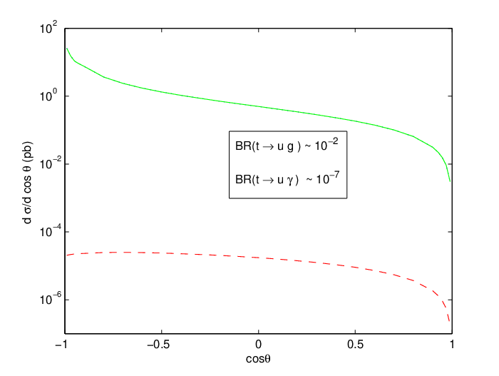
Is there a way, then, to ascertain whether the main contribution to σ⁡(p​p→u​g→t​γ)\sigma(p\,p\rightarrow ug\rightarrow t\,\gamma) stems from anomalous strong interactions, or from weak ones? Indeed there is, by analysing the differential cross section for this process. In fig. (9) we plot d​σ/d​cos⁡θd\sigma/d\cos\theta versus

Refer to caption
Figure 9: Differential cross section p​p→u​g→t​γp\,p\rightarrow\,u\,g\rightarrow t\,\gamma versus cos⁡θ\cos\theta, for a typical choice of parameters with a branching ratio for t→u​gt\,\rightarrow\,u\,g much larger than B​r​(t→u​γ)Br(t\,\rightarrow\,u\,\gamma). The strong contribution practically coincides with the total cross section (full line). The electroweak contribution is represented by the dashed line.

cos⁡θ\cos\theta, θ\theta being the angle between the momentum of the photon (or top) and the beam line. We show the strong and electroweak contributions to this cross section, as well as its total result. We chose a typical set of values for the anomalous couplings producing a branching ratio for the FCNC decay t→u​gt\,\rightarrow\,u\,g clearly superior to that of the decay t→u​γt\,\rightarrow\,u\,\gamma. As we see, the angular distribution of the electroweak and strong cross sections is quite different. Since the strong anomalous interactions are dominating over the electroweak ones the total cross section mimics very closely the strong one.
Refer to caption
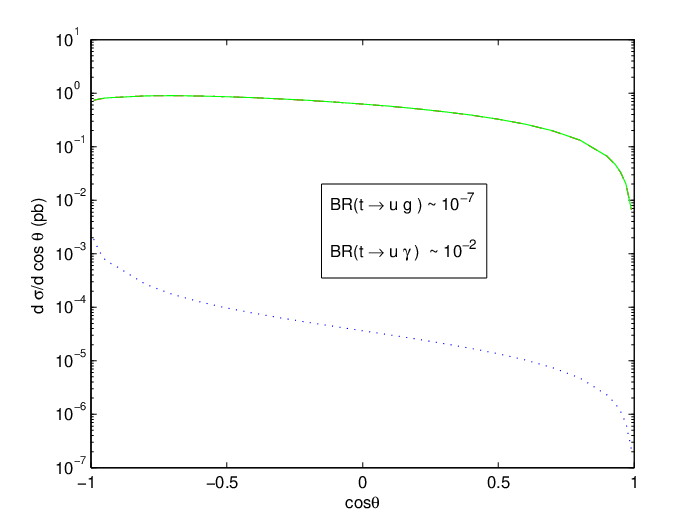
Figure 10: Differential cross section p​p→u​g→t​γp\,p\rightarrow\,u\,g\rightarrow t\,\gamma versus cos⁡θ\cos\theta, for a typical choice of parameters with a branching ratio for t→u​gt\,\rightarrow\,u\,g much smaller than B​r​(t→u​γ)Br(t\,\rightarrow\,u\,\gamma). The electroweak contribution practically coincides with the total cross section (full line). The strong contribution is represented by the dotted line.

In fig. (10) we show the inverse situation: a typical set of values was chosen which gives us B​r​(t→u​γ)∼ 10−2Br(t\,\rightarrow\,u\,\gamma)\,\sim\,10^{-2} and B​r​(t→u​g)∼ 10−7Br(t\,\rightarrow\,u\,g)\,\sim\,10^{-7}, meaning a situation for which the anomalous electroweak interactions are clearly dominant over the strong ones. We see from the angular distribution of the total cross section shown in fig. (10) that it now greatly resembles its electroweak component. Judging from figs. (9) and (10), the telltale sign of dominance of strong FCNC interactions is a pronounced variation with cos⁡θ\cos\theta in the cross section, whereas a dominance of electroweak FCNC effects will produce a relatively “flat” cross section. The Feynman diagrams of fig. (6) help to explain this difference in dependence with cos⁡θ\cos\theta: the strong cross section has a significant contribution from the tt-channel (since the ss-channel diagram is suppressed by the top mass), whereas the inverse happens for the electroweak cross section. However, it should be pointed out that the four-legged diagrams contributing to both cross sections will upset a clear ss-or-tt channel dominance. Notice also that if FCNC produce branching ratios of similar size in both sectors the difference in behaviour shown in these plots will not be seen. In fact, we may get a better feel for the different angular behavior of the strong and electroweak FCNC interactions if we define an asymmetry coefficient for this cross section,

At+γ=σt+γ​(cos⁡θ>0)−σt+γ​(cos⁡θ<0)σt+γ​(cos⁡θ>0)+σt+γ​(cos⁡θ<0).A_{t+\gamma}\;=\;\frac{\sigma_{t+\gamma}(\cos\theta>0)\,-\,\sigma_{t+\gamma}(\cos\theta<0)}{\sigma_{t+\gamma}(\cos\theta>0)\,+\,\sigma_{t+\gamma}(\cos\theta<0)}\;\;\;. (20)

To exemplify the relevance of this quantity, we generated a special sample of anomalous couplings: random values of all strong and electroweak couplings such that B​r​(t→u​γ)+B​r​(t→u​g)∼10−2Br(t\,\rightarrow\,u\,\gamma)\,+\,Br(t\,\rightarrow\,u\,g)\sim 10^{-2}. This will include the cases where one of the branching ratios dominates over the other, and also the case where both of them have similar magnitudes. We show the results in fig. (11), plotting the value of At+γA_{t+\gamma} in

Refer to caption
Figure 11: The angular asymmetry coefficient defined in eq. (20) as a function of the branching ratios B​r​(t→u​γ)Br(t\,\rightarrow\,u\,\gamma) (crosses) and B​r​(t→u​g)Br(t\,\rightarrow\,u\,g) (dots).

terms of the two branching ratios whose sum is fixed to 10−210^{-2}. Looking at the far left of the plot we see that when the electroweak FCNC interactions dominate over the strong ones At+γA_{t+\gamma} tends to a value of approximately −0.85-0.85, and in the reverse situation we have At+γ∼−0.42A_{t+\gamma}\,\sim\,-0.42. However, when both branching ratios have similar sizes, At+γA_{t+\gamma} can take any value between those two limits.

IV.2 Cross section for q​g→t​Zq\,g\rightarrow t\,Z

We can perform analysis similar to those of the previous section for the associated production of a top and a Z boson. We computed an analytical expression for the cross section of this process, which is given by the sum of three terms,

d​σq​g→t​Zd​t=d​σq​g→t​ZE​Wd​t+d​σq​g→t​ZSd​t+d​σq​g→t​ZI​n​td​t,\frac{d\sigma_{qg\rightarrow tZ}}{dt}\;=\;\frac{d\sigma^{EW}_{qg\rightarrow tZ}}{dt}\;+\;\frac{d\sigma^{S}_{qg\rightarrow tZ}}{dt}\;+\;\frac{d\sigma^{Int}_{qg\rightarrow tZ}}{dt}\;\;\;, (21)

with strong FCNC contributions (σS\sigma^{S}), electroweak ones (σE​W\sigma^{EW}) and interference terms between both sectors. The expression for d​σq​g→t​ZS/d​td\sigma^{S}_{qg\rightarrow tZ}/dt was first given in ref. [4]. The remaining formulae are quite lengthy, involving many different combinations of anomalous couplings with complicated coefficients. We present them in Appendix A for completeness. To examine the values of these cross sections at the LHC, we used the set of anomalous couplings generated in the previous section, complemented with randomly generated values for the η\eta and θ\theta couplings 44 4 Which, recall, do not contribute to FCNC interactions involving the photon, only the Z. and integrated the expressions (21) with the CTEQ6M pdf’s. We chose μF=mt+mZ\mu_{F}\,=\,m_{t}\,+\,m_{Z} and imposed a 10 GeV cut on the transverse momentum of the particles in the final state.

Refer to caption
Figure 12: Total (electroweak and strong contributions) cross section for the process p​p→u​g→t​Zp\,p\rightarrow\,u\,g\rightarrow t\,Z versus the sum of the FCNC branching ratios for the decays t→u​Zt\,\rightarrow\,u\,Z and t→u​gt\,\rightarrow\,u\,g.

Unlike what was observed for the t​γt\,\gamma channel, there is no direct proportionality between σE​W​(p​p→u​g→t​Z)\sigma^{EW}(pp\rightarrow ug\rightarrow tZ) and B​r​(t→q​Z)Br(t\,\rightarrow\,q\,Z) - this is due to the many different functions multiplying the several combinations of anomalous couplings presented in Appendix A. Because the functions F1ZF_{1_{Z}} and F2ZF_{2_{Z}} (eqs. (26)) are very similar, there is an approximate proportionality between the branching ratio and σS​(p​p→u​g→t​Z)\sigma^{S}(pp\rightarrow ug\rightarrow tZ), as was seen in ref. [4]. In fig. (12) we plot the total cross section for this process against the sum B​r​(t→u​Z)+B​r​(t→u​g)Br(t\,\rightarrow\,u\,Z)\,+\,Br(t\,\rightarrow\,u\,g). We see, from this plot, that the cross section for t+Zt\,+\,Z production is always contained between two straight lines, and it is easy to obtain the following relation, valid for the overwhelming majority of the points shown in fig. (12):

200​[B​r​(t→u​g)+B​r​(t→u​Z)]<σ⁡(p​p→u​g→t​Z)< 104​[B​r​(t→u​g)+B​r​(t→u​Z)]​(pb).200\,\left[Br(t\rightarrow u\,g)\,+\,Br(t\rightarrow u\,Z)\right]\,<\,\sigma(pp\rightarrow u\,g\rightarrow t\,Z)\,<\,10^{4}\,\left[Br(t\rightarrow u\,g)\,+\,Br(t\rightarrow u\,Z)\right]\,\mbox{(pb)}. (22)

The thick band observed in this figure means any bounds obtained, say, on the cross section, will translate into a less severe bound on the sum of the branching ratios than what happened for the t+γt\,+\,\gamma channel. For instance, in fig. (8) an upper bound on the cross section σ⁡(p​p→u​g→t​γ)\sigma(pp\rightarrow ug\rightarrow t\gamma) of 10−210^{-2} implied B​r​(t→u​γ)+B​r​(t→u​g)< 10−5Br(t\,\rightarrow\,u\,\gamma)\,+\,Br(t\,\rightarrow\,u\,g)\,<\,10^{-5}, whereas a similar bound on σ⁡(p​p→u​g→t​Z)\sigma(pp\rightarrow ug\rightarrow tZ) gives us approximately, from the right-hand side of the band in fig. (12), B​r​(t→u​Z)+B​r​(t→u​g)< 10−4Br(t\,\rightarrow\,u\,Z)\,+\,Br(t\,\rightarrow\,u\,g)\,<\,10^{-4}. If we didn’t have this band of values, but rather a line corresponding to its left-hand side edge, the bound would be one order of magnitude lower. As before, we obtain qualitatively identical results for the processes involving the cc quark, and we can quote rough bounds similar to those of eq. (22),

30​[B​r​(t→c​g)+B​r​(t→c​Z)]<σ⁡(p​p→c​g→t​Z)< 600​[B​r​(t→c​g)+B​r​(t→c​Z)]​(pb).30\,\left[Br(t\rightarrow c\,g)\,+\,Br(t\rightarrow c\,Z)\right]\,<\,\sigma(pp\rightarrow c\,g\rightarrow t\,Z)\,<\,600\,\left[Br(t\rightarrow c\,g)\,+\,Br(t\rightarrow c\,Z)\right]\,\mbox{(pb)}. (23)
Refer to caption
Figure 13: Differential cross sections for the process p​p→u​g→t​Zpp\rightarrow ug\rightarrow tZ. Total (thick line), electroweak (dashed line) and strong (dotted line) contributions. The electroweak contribution practically coincides with the strong one.

And again, we observe that the strong and electroweak cross sections have different angular dependencies. In fig. (13) we plot the differential cross section for the process p​p→u​g→t​Zpp\rightarrow ug\rightarrow tZ, both the strong and electroweak contributions, for a typical choice of anomalous couplings for which the electroweak FCNC interactions dominate over the strong ones. The strong contributions increase with cos⁡θ\cos\theta, whereas the electroweak ones decrease. If the strong FCNC couplings dominate over the electroweak ones, then the total cross section would very closely mimic the angular dependence of the dotted line in fig. (13). Once more, if the electroweak and strong FCNC interactions have contributions of similar magnitudes, then it will not be possible to distinguish them through this analysis. We can define an asymmetry coefficient for the t+Zt\,+\,Z process as well, namely

At+Z=σt+Z​(cos⁡θ>0)−σt+Z​(cos⁡θ<0)σt+Z​(cos⁡θ>0)+σt+Z​(cos⁡θ<0).A_{t+Z}\;=\;\frac{\sigma_{t+Z}(\cos\theta>0)\,-\,\sigma_{t+Z}(\cos\theta<0)}{\sigma_{t+Z}(\cos\theta>0)\,+\,\sigma_{t+Z}(\cos\theta<0)}\;\;\;. (24)

We will now use the set of anomalous couplings generated to produce fig. (11) and plot the evolution of At+ZA_{t+Z} with both FCNC branching ratios in fig. (14).

Refer to caption
Figure 14: The angular asymmetry coefficient At+ZA_{t+Z} as a function of the branching ratios B​r​(t→u​Z)Br(t\,\rightarrow\,u\,Z) (crosses) and B​r​(t→u​g)Br(t\,\rightarrow\,u\,g) (dots).

Again, we see a clear distinction between dominance of electroweak FCNC interactions or strong FCNC ones. In the former case At+ZA_{t+Z} tends to a value of approximately 0.40.4, and in the latter situation we have At+Z∼−0.4A_{t+Z}\,\sim\,-0.4 - this is particulary interesting since the asymmetry changes signs, going from one regime to the other. Once more, if both branching ratios have like sizes, At+ZA_{t+Z} may have any value between these two extrema.

V Discussion and conclusions

Even if the top quark has indeed large FCNC branching ratios - strong or electroweak ones -, which would lead to significant cross sections of associated single top production at the LHC, could those processes actually be observed? In other words, given the numerous backgrounds present at the LHC, is it possible to extract a meaningful FCNC signal from the expected data? The very thorough analysis of ref. [7] seems to indicate so. For instance, for t+Zt\,+\,Z production they identify several possible channels available to identify the FCNC signal, summarised in table 3.

Final State Fraction (%) Backgrounds
t​Z→(b​j​j)​(j​j)tZ\rightarrow(bjj)\,(jj) 22.2 j​j​j​j​jjjjjj
t​Z→(b​j​j)​(ν​ν¯)tZ\rightarrow(bjj)\,(\nu\bar{\nu}) 8.1 t​t¯t\bar{t}, W​tWt, Z​j​j​jZjjj
t​Z→(b​l​ν)​(j​j)tZ\rightarrow(bl\nu)\,(jj) 7.5 t​t¯t\bar{t}, W​tWt, W​j​j​jWjjj
t​Z→(b​l​ν)​(ν​ν¯)tZ\rightarrow(bl\nu)\,(\nu\bar{\nu}) 2.7 W​jWj
t​Z→(b​j​j)​(l​l)tZ\rightarrow(bjj)\,(ll) 2.3 Z​j​j​jZjjj, Z​W​jZWj
t​Z→(b​j​j)​(b¯​b)tZ\rightarrow(bjj)\,(\bar{b}b) 2.2 b​b¯​j​j​jb\bar{b}jjj
t​Z→(b​l​ν)​(l​l)tZ\rightarrow(bl\nu)\,(ll) 0.8 Z​W​jZWj
t​Z→(b​l​ν)​(b¯​b)tZ\rightarrow(bl\nu)\,(\bar{b}b) 0.7 t​t¯t\bar{t}, W​tWt, Z​W​jZWj, W​b​b¯​jWb\bar{b}j
Table 3: Possible final states in t​Zt\,Z production, and main backgrounds to each process [7].

For all of these processes, the processes W​Z​jWZj, t​t¯t\bar{t} and single top production will also act as backgrounds. It is also likely, considering the immense QCD backgrounds, that only those processes with at least one lepton will be possible to observe at the LHC. To build this table, the top quark was considered to decay according to SM physics, t→b​Wt\rightarrow b\,W, and the several decay possibilities within the SM of the WW and ZZ bosons give the possibilities listed therein. The fraction attributed to each channel corresponds to the percentages of each decay mode of the WW and ZZ as well as a 90 % tagging efficiency for lepton (electron or muon) tagging, and a 60 % one for each b-jet. The most impressive result of ref. [7], though, is the efficiency with which the FCNC signal is extracted from these backgrounds: they have shown that a battery of simple kinematical cuts on the observed particles is more than enough to obtain a very clear - and statistically meaningful - FCNC signal. For t+Zt\,+\,Z production they conclude that the best channel would be p​p→t​Z→l+​l−​l​ν​bp\,p\rightarrow t\,Z\rightarrow l^{+}\,l^{-}\,l\,\nu\,b. For t+γt\,+\,\gamma production the analysis is made simpler by the photon not having decay branching ratios, which aides the statistics obtained - the best channel available would be p​p→t​γ→γ​l​ν​bp\,p\rightarrow t\,\gamma\rightarrow\gamma\,l\,\nu\,b. Clearly, only an analysis analogous to that of [7], with the FCNC interactions considered in the present paper included in an event generator, would be capable of reaching definite conclusions regarding which kinematical cuts would be better suited to obtain a clear FCNC signal. That study is beyond the scope of the present paper, though a preliminary study of our strong FCNC interactions in the LHC environment, using the TopReX event generator [25], is about to be concluded [26]. A word on higher-order QCD corrections: they are manifestly difficult to compute in the effective operator formalism, since the lagrangian becomes non-renormalizable. A recent work using electroweak top FCNC couplings [27], however, concluded that those corrections greatly reduce any dependence the results obtained at tree level might have on the scales of renormalization and factorization. These authors have also shown that the higher order corrections tend to slightly increase the leading order result.

To summarise, we employed the effective operator formalism to parameterize the effects of any theory that might have as its low-energy limit the SM. The fact that we are working in a gauge invariant formalism allowed us to find many relations between couplings and quantities which, a priori, would not be related at all. In particular we found a near-proportionality between the cross section of associated top plus photon production at the LHC and the sum of the FCNC decays of the top to a photon and a gluon. We estimated the cross sections for t+γt\,+\,\gamma and t+Zt\,+\,Z production at the LHC and saw that, for large enough values of the top FCNC branching ratios, one might expect a significant number of events. We also concluded that, for these processes, the interplay between the strong and electroweak anomalous interactions tends to increase the values of the cross sections - the interference between both FCNC sectors is mostly constructive. The analysis of the differential cross sections for t+γt\,+\,\gamma and t+Zt\,+\,Z production will possibly allow the identification of the source of FCNC physics - the strong or the electroweak sector.

Acknowledgments: Our thanks to Nuno Castro, Filipe Veloso and António Onofre for a careful reading of the manuscript and many interesting discussions. This work is supported by Fundação para a Ciência e Tecnologia under contract POCI/FIS/59741/2004 and PTDC/FIS/70156/2006. R.S. is supported by FCT under contract SFRH/BPD/23427/2005. R.G.J. is supported by FCT under contract SFRH/BD/19781/2004.

Appendix A Cross section expression for the process q​g→t​Zq\,g\rightarrow t\,Z

As mentioned in section IV.2 the cross section for the associated production of a top and a Z boson is given by three terms, as in eq. (21). The strong FCNC contribution is given by:

d​σq​g→t​ZSd​t\displaystyle\frac{d\,\sigma^{S}_{q\,g\rightarrow t\,Z}}{dt} =\displaystyle= e296​π​s2​Λ4[F1Z(t,s){|αq​tS+(αt​qS)∗|2+8​vmtIm[(αq​tS+(αt​qS)∗)βt​qS]+16​v2mt2|βt​qS|2}+\displaystyle\frac{e^{2}}{96\,\pi\,s^{2}\,\Lambda^{4}}\left[F_{1_{Z}}(t,s)\,\left\{\left|\alpha^{S}_{qt}+(\alpha^{S}_{tq})^{*}\right|^{2}+\frac{8v}{m_{t}}\,Im\left[(\alpha^{S}_{qt}+(\alpha^{S}_{tq})^{*})\,\beta^{S}_{tq}\right]+\frac{16v^{2}}{m_{t}^{2}}\,\left|\beta^{S}_{tq}\right|^{2}\right\}+\right. (25)
+F2Z(t,s)16​v2mt2|βq​tS|2],\displaystyle\qquad\qquad\left.+\,F_{2_{Z}}(t,s)\,\frac{16v^{2}}{m_{t}^{2}}\,\left|\beta^{S}_{qt}\right|^{2}\right]\;\;\;,

with coefficients

F1Z​(t,s)\displaystyle F_{1_{Z}}(t,s) =\displaystyle= −mt272​cW2​mZ2​(mt2−s)2​sW2​t2[32mt8mZ2sW4(mZ2−t)+32mt4mZ2sW4(mZ2−t)(s2+4st+t2)+\displaystyle\frac{-m_{t}^{2}}{72\,c_{W}^{2}\,m_{Z}^{2}\,{\left(m_{t}^{2}-s\right)}^{2}\,s_{W}^{2}\,t^{2}}\left[32\,m_{t}^{8}\,m_{Z}^{2}\,s_{W}^{4}\,\left(m_{Z}^{2}-t\right)+32\,m_{t}^{4}\,m_{Z}^{2}\,s_{W}^{4}\,\left(m_{Z}^{2}-t\right)\,\left(s^{2}+4\,s\,t+t^{2}\right)+\right.
s2​t2​(2​mZ4​(9−24​sW2+32​sW4)+9​s​t−2​mZ2​(9−24​sW2+32​sW4)​(s+t))+\displaystyle\qquad\qquad s^{2}\,t^{2}\,\left(2\,m_{Z}^{4}\,\left(9-24\,s_{W}^{2}+32\,s_{W}^{4}\right)+9\,s\,t-2\,m_{Z}^{2}\,\left(9-24\,s_{W}^{2}+32\,s_{W}^{4}\right)\,\left(s+t\right)\right)\,+
mt2​s​t​(−9​s​t2−64​mZ4​sW4​(s+t)+mZ2​(32​s2​sW4+3​s​(3−32​sW2+64​sW4)​t+96​sW4​t2))−\displaystyle\qquad\qquad m_{t}^{2}\,s\,t\,\left(-9\,s\,t^{2}-64\,m_{Z}^{4}\,s_{W}^{4}\,\left(s+t\right)+m_{Z}^{2}\,\left(32\,s^{2}\,s_{W}^{4}+3\,s\,\left(3-32\,s_{W}^{2}+64\,s_{W}^{4}\right)\,t+96\,s_{W}^{4}\,t^{2}\right)\right)-
32mt6mZ2sW4(2mZ2(s+t)−t(s+2t))]\displaystyle\qquad\qquad\left.32\,m_{t}^{6}\,m_{Z}^{2}\,s_{W}^{4}\,\left(2\,m_{Z}^{2}\,\left(s+t\right)-t\,\left(s+2\,t\right)\right)\right]
F2Z​(t,s)\displaystyle F_{2_{Z}}(t,s) =\displaystyle= mt272​cW2​mZ2​(mt2−s)2​sW2​t2[−2mt4mZ2(3−4sW2)2(mZ2−t)(s2+4st+t2)+\displaystyle\frac{m_{t}^{2}}{72\,c_{W}^{2}\,m_{Z}^{2}\,{\left(m_{t}^{2}-s\right)}^{2}\,s_{W}^{2}\,t^{2}}\left[-2\,m_{t}^{4}\,m_{Z}^{2}\,{\left(3-4\,s_{W}^{2}\right)}^{2}\,\left(m_{Z}^{2}-t\right)\,\left(s^{2}+4\,s\,t+t^{2}\right)+\right. (26)
s2​t2​(−2​mZ4​(9−24​sW2+32​sW4)−9​s​t+2​mZ2​(9−24​sW2+32​sW4)​(s+t))+\displaystyle\qquad\qquad s^{2}\,t^{2}\,\left(-2\,m_{Z}^{4}\,\left(9-24\,s_{W}^{2}+32\,s_{W}^{4}\right)-9\,s\,t+2\,m_{Z}^{2}\,\left(9-24\,s_{W}^{2}+32\,s_{W}^{4}\right)\,\left(s+t\right)\right)+
mt2st{9st2+4mZ4(3−4sW2)2(s+t)+mZ2(−2s2(3−4sW2)2−\displaystyle\qquad\qquad m_{t}^{2}\,s\,t\,\left\{9\,s\,t^{2}+4\,m_{Z}^{4}\,{\left(3-4\,s_{W}^{2}\right)}^{2}\,\left(s+t\right)+m_{Z}^{2}\,\left(-2\,s^{2}\,{\left(3-4\,s_{W}^{2}\right)}^{2}\right.-\right.
3s(15+64(−sW2+sW4))t−6(3−4sW2)2t2)}\displaystyle\qquad\qquad\left.\left.3\,s\,\left(15+64\,\left(-s_{W}^{2}+s_{W}^{4}\right)\right)\,t-6\,{\left(3-4\,s_{W}^{2}\right)}^{2}\,t^{2}\right)\right\}
2mt8mZ2(3−4sW2)2(−mZ2+t)+2mt6mZ2(3−4sW2)2(2mZ2(s+t)−t(s+2t))].\displaystyle\qquad\qquad\left.2\,m_{t}^{8}\,m_{Z}^{2}\,{\left(3-4\,s_{W}^{2}\right)}^{2}\,\left(-m_{Z}^{2}+t\right)+2\,m_{t}^{6}\,m_{Z}^{2}\,{\left(3-4\,s_{W}^{2}\right)}^{2}\,\left(2\,m_{Z}^{2}\,\left(s+t\right)-t\,\left(s+2\,t\right)\right)\right]\;\;\;.

The electroweak FCNC contribution is given by the following expression:

d​σq​g→t​ZE​Wd​t\displaystyle\frac{d\,\sigma^{EW}_{q\,g\rightarrow t\,Z}}{dt} =\displaystyle= gs296​π​s2​Λ4[G1Z(t,s)|αq​tZ|2+G2Z(t,s)|αt​qZ|2+G3Z(t,s)(|βq​tZ|2+|βt​qZ|2)+G4Z(t,s)(|ηq​t|2+|η¯q​t|2)\displaystyle\frac{g_{s}^{2}}{96\,\pi\,s^{2}\,\Lambda^{4}}\left[G_{1_{Z}}(t,s)\,\left|\alpha^{Z}_{qt}\right|^{2}+G_{2_{Z}}(t,s)\,\left|\alpha^{Z}_{tq}\right|^{2}+G_{3_{Z}}(t,s)\,(\left|\beta^{Z}_{qt}\right|^{2}+\left|\beta^{Z}_{tq}\right|^{2})+G_{4_{Z}}(t,s)\,(\left|\eta_{qt}\right|^{2}+\left|\bar{\eta}_{qt}\right|^{2})\right. (27)
+G5Z​(t,s)​|θ|2+G6Z​(t,s)​R​e​[αq​tZ​αt​qZ]+G7Z​(t,s)​I​m​[αq​tZ​βt​qZ]\displaystyle\qquad+\,G_{5_{Z}}(t,s)\,\left|\theta\right|^{2}+G_{6_{Z}}(t,s)\,Re\left[\alpha^{Z}_{qt}\,\alpha^{Z}_{tq}\right]+G_{7_{Z}}(t,s)\,Im\left[\alpha^{Z}_{qt}\,\beta^{Z}_{tq}\right]
+G8Z​(t,s)​I​m​[αt​qZ∗​βt​qZ]+G9Z​(t,s)​R​e​[αq​tZ​θ∗]+G10Z​(t,s)​R​e​[αt​qZ​θ]\displaystyle\qquad+\,G_{8_{Z}}(t,s)\,Im\left[\alpha^{Z^{*}}_{tq}\,\beta^{Z}_{tq}\right]+G_{9_{Z}}(t,s)\,Re\left[\alpha^{Z}_{qt}\theta^{*}\right]+G_{10_{Z}}(t,s)\,Re\left[\alpha^{Z}_{tq}\theta\right]
+G11Z(t,s)Re[βq​tZ(ηq​t−η¯q​t)∗]+G12Z(t,s)Im[βt​qZθ]+G13Z(t,s)Re[ηq​tη¯q​t∗]]\displaystyle\qquad\left.+\,G_{11_{Z}}(t,s)\,Re\left[\beta^{Z}_{qt}(\eta_{qt}-\bar{\eta}_{qt})^{*}\right]+G_{12_{Z}}(t,s)\,Im\left[\beta^{Z}_{tq}\,\theta\right]+G_{13_{Z}}(t,s)\,Re\left[\eta_{qt}\bar{\eta}_{qt}^{*}\right]\right]

where the GiZG_{i_{Z}} functions are given by

G1Z​(t,s)\displaystyle G_{1_{Z}}(t,s) =\displaystyle= 14​s​(mt2−t)2[mt10+mt8(2mZ2−2s−t)+mt6(−5mZ4+s2+4st+t2−4mZ2(s+t))\displaystyle\frac{1}{4\,s\,{\left(m_{t}^{2}-t\right)}^{2}}\left[m_{t}^{10}+m_{t}^{8}\,\left(2\,m_{Z}^{2}-2\,s-t\right)+m_{t}^{6}\,\left(-5\,m_{Z}^{4}+s^{2}+4\,s\,t+t^{2}-4\,m_{Z}^{2}\,\left(s+t\right)\right)\right.
+mt2​(2​mZ8−8​mZ6​t−4​mZ2​t2​(s+t)+2​s​t2​(s+t)+mZ4​(s+3​t)2)\displaystyle+m_{t}^{2}\,\left(2\,m_{Z}^{8}-8\,m_{Z}^{6}\,t-4\,m_{Z}^{2}\,t^{2}\,\left(s+t\right)+2\,s\,t^{2}\,\left(s+t\right)+m_{Z}^{4}\,{\left(s+3\,t\right)}^{2}\right)
−mZ4t(2mZ4+s2+t2−2mZ2(s+t))+mt4(6mZ6−3mZ4t+2mZ2t(s+3t)−t(3s2+6st+t2))]\displaystyle\left.-m_{Z}^{4}\,t\,\left(2\,m_{Z}^{4}+s^{2}+t^{2}-2\,m_{Z}^{2}\,\left(s+t\right)\right)+m_{t}^{4}\,\left(6\,m_{Z}^{6}-3\,m_{Z}^{4}\,t+2\,m_{Z}^{2}\,t\,\left(s+3\,t\right)-t\,\left(3\,s^{2}+6\,s\,t+t^{2}\right)\right)\right]
G2Z​(t,s)\displaystyle G_{2_{Z}}(t,s) =\displaystyle= 14​s​(mt2−t)2[mt10−mt8(4mZ2+2s+t)+mt6(7mZ4+s2+2mZ2t+4st+t2)\displaystyle\frac{1}{4\,s\,{\left(m_{t}^{2}-t\right)}^{2}}\left[m_{t}^{10}-m_{t}^{8}\,\left(4\,m_{Z}^{2}+2\,s+t\right)+m_{t}^{6}\,\left(7\,m_{Z}^{4}+s^{2}+2\,m_{Z}^{2}\,t+4\,s\,t+t^{2}\right)\right.
−mZ4​t​(2​mZ4+s2+t2−2​mZ2​(s+t))−mt4​(6​mZ6+3​mZ4​t−2​mZ2​s​(s+3​t)+t⁡(3​s2+6​s​t+t2))\displaystyle-m_{Z}^{4}\,t\,\left(2\,m_{Z}^{4}+s^{2}+t^{2}-2\,m_{Z}^{2}\,\left(s+t\right)\right)-m_{t}^{4}\,\left(6\,m_{Z}^{6}+3\,m_{Z}^{4}\,t-2\,m_{Z}^{2}\,s\,\left(s+3\,t\right)+t\,\left(3\,s^{2}+6\,s\,t+t^{2}\right)\right)
+mt2(2mZ8+4mZ6t+2st2(s+t)+mZ4(s2−6st−3t2)+mZ2(−2s2t+2t3))]\displaystyle\left.+m_{t}^{2}\,\left(2\,m_{Z}^{8}+4\,m_{Z}^{6}\,t+2\,s\,t^{2}\,\left(s+t\right)+m_{Z}^{4}\,\left(s^{2}-6\,s\,t-3\,t^{2}\right)+m_{Z}^{2}\,\left(-2\,s^{2}\,t+2\,t^{3}\right)\right)\right]
G3Z​(t,s)\displaystyle G_{3_{Z}}(t,s) =\displaystyle= 2​v2s​(mt2−t)2[2mt8−mt6(3mZ2+4s+2t)−t(2mZ6−2mZ4(s+t)−4st(s+t)+mZ2(s+t)2)\displaystyle\frac{2\,v^{2}}{s\,{\left(m_{t}^{2}-t\right)}^{2}}\left[2\,m_{t}^{8}-m_{t}^{6}\,\left(3\,m_{Z}^{2}+4\,s+2\,t\right)-t\,\left(2\,m_{Z}^{6}-2\,m_{Z}^{4}\,\left(s+t\right)-4\,s\,t\,\left(s+t\right)+m_{Z}^{2}\,{\left(s+t\right)}^{2}\right)\right.
+mt4​(2​mZ4−mZ2​(2​s+t)+2​(s2+4​s​t+t2))\displaystyle+m_{t}^{4}\,\left(2\,m_{Z}^{4}-m_{Z}^{2}\,\left(2\,s+t\right)+2\,\left(s^{2}+4\,s\,t+t^{2}\right)\right)
+mt2(2mZ6−4mZ4t−2t(3s2+6st+t2)+mZ2(s2+6st+5t2))]\displaystyle\left.+m_{t}^{2}\,\left(2\,m_{Z}^{6}-4\,m_{Z}^{4}\,t-2\,t\,\left(3\,s^{2}+6\,s\,t+t^{2}\right)+m_{Z}^{2}\,\left(s^{2}+6\,s\,t+5\,t^{2}\right)\right)\right]
G4Z​(t,s)\displaystyle G_{4_{Z}}(t,s) =\displaystyle= v28​mZ2​s​(mt2−t)2[mt10−mt8(4mZ2+2s+t)+mt6(7mZ4+2mZ2t+(s+t)2)\displaystyle\frac{v^{2}}{8\,m_{Z}^{2}\,s\,{\left(m_{t}^{2}-t\right)}^{2}}\left[m_{t}^{10}-m_{t}^{8}\,\left(4\,m_{Z}^{2}+2\,s+t\right)+m_{t}^{6}\,\left(7\,m_{Z}^{4}+2\,m_{Z}^{2}\,t+{\left(s+t\right)}^{2}\right)\right.
−mZ2​t​(2​mZ6−2​mZ4​(s+t)−4​s​t​(s+t)+mZ2​(s+t)2)\displaystyle-m_{Z}^{2}\,t\,\left(2\,m_{Z}^{6}-2\,m_{Z}^{4}\,\left(s+t\right)-4\,s\,t\,\left(s+t\right)+m_{Z}^{2}\,{\left(s+t\right)}^{2}\right)
−mt4​(6​mZ6+t​(s+t)2+mZ4​(2​s+3​t)−2​mZ2​s​(3​s+5​t))\displaystyle-m_{t}^{4}\,\left(6\,m_{Z}^{6}+t\,{\left(s+t\right)}^{2}+m_{Z}^{4}\,\left(2\,s+3\,t\right)-2\,m_{Z}^{2}\,s\,\left(3\,s+5\,t\right)\right)
+mt2mZ2(2mZ6+4mZ4t+mZ2(s2−2st−3t2)+2t(−5s2−4st+t2))]\displaystyle\left.+m_{t}^{2}\,m_{Z}^{2}\,\left(2\,m_{Z}^{6}+4\,m_{Z}^{4}\,t+m_{Z}^{2}\,\left(s^{2}-2\,s\,t-3\,t^{2}\right)+2\,t\,\left(-5\,s^{2}-4\,s\,t+t^{2}\right)\right)\right]
G5Z​(t,s)\displaystyle G_{5_{Z}}(t,s) =\displaystyle= v42​mZ2​s​(mt2−t)2[mt8−mt6(2s+t)−2mZ2t(2mZ4+s2+t2−2mZ2(s+t))\displaystyle\frac{v^{4}}{2\,m_{Z}^{2}\,s\,{\left(m_{t}^{2}-t\right)}^{2}}\left[m_{t}^{8}-m_{t}^{6}\,\left(2\,s+t\right)-2\,m_{Z}^{2}\,t\,\left(2\,m_{Z}^{4}+s^{2}+t^{2}-2\,m_{Z}^{2}\,\left(s+t\right)\right)\right.
+mt4(−2mZ4−2mZ2t+(s+t)2)+mt2(4mZ6−2mZ4t−t(s+t)2+2mZ2(s2−st+2t2))]\displaystyle\left.+m_{t}^{4}\,\left(-2\,m_{Z}^{4}-2\,m_{Z}^{2}\,t+{\left(s+t\right)}^{2}\right)+m_{t}^{2}\,\left(4\,m_{Z}^{6}-2\,m_{Z}^{4}\,t-t\,{\left(s+t\right)}^{2}+2\,m_{Z}^{2}\,\left(s^{2}-s\,t+2\,t^{2}\right)\right)\right]
G6Z​(t,s)\displaystyle G_{6_{Z}}(t,s) =\displaystyle= 12​s​(mt2−t)2[mt10−mt8(2mZ2+2s+t)+mt6(mZ4+s2+4st+t2)\displaystyle\frac{1}{2\,s\,{\left(m_{t}^{2}-t\right)}^{2}}\left[m_{t}^{10}-m_{t}^{8}\,\left(2\,m_{Z}^{2}+2\,s+t\right)+m_{t}^{6}\,\left(m_{Z}^{4}+s^{2}+4\,s\,t+t^{2}\right)\right.
+mZ4​t​(2​mZ4+s2+t2−2​mZ2​(s+t))−mt2​(2​mZ8+mZ4​(s−t)2−2​s​t2​(s+t))\displaystyle+m_{Z}^{4}\,t\,\left(2\,m_{Z}^{4}+s^{2}+t^{2}-2\,m_{Z}^{2}\,\left(s+t\right)\right)-m_{t}^{2}\,\left(2\,m_{Z}^{8}+m_{Z}^{4}\,{\left(s-t\right)}^{2}-2\,s\,t^{2}\,\left(s+t\right)\right)
+mt4(2mZ6−mZ4t+2mZ2t(s+t)−t(3s2+6st+t2))]\displaystyle\left.+m_{t}^{4}\,\left(2\,m_{Z}^{6}-m_{Z}^{4}\,t+2\,m_{Z}^{2}\,t\,\left(s+t\right)-t\,\left(3\,s^{2}+6\,s\,t+t^{2}\right)\right)\right]
G7Z​(t,s)\displaystyle G_{7_{Z}}(t,s) =\displaystyle= 2​mt​vs​(mt2−t)2[mt8−mt6(2s+t)+mt4(−2mZ4+s2+4st+t2−2mZ2(s+t))\displaystyle\frac{2\,m_{t}\,v}{s\,{\left(m_{t}^{2}-t\right)}^{2}}\left[m_{t}^{8}-m_{t}^{6}\,\left(2\,s+t\right)+m_{t}^{4}\,\left(-2\,m_{Z}^{4}+s^{2}+4\,s\,t+t^{2}-2\,m_{Z}^{2}\,\left(s+t\right)\right)\right.
+2​t​(−2​mZ6+2​mZ4​(s+t)−mZ2​t​(s+t)+s​t​(s+t))\displaystyle+2\,t\,\left(-2\,m_{Z}^{6}+2\,m_{Z}^{4}\,\left(s+t\right)-m_{Z}^{2}\,t\,\left(s+t\right)+s\,t\,\left(s+t\right)\right)
+mt2(4mZ6−2mZ4t+2mZ2t(s+2t)−t(3s2+6st+t2))]\displaystyle\left.+m_{t}^{2}\,\left(4\,m_{Z}^{6}-2\,m_{Z}^{4}\,t+2\,m_{Z}^{2}\,t\,\left(s+2\,t\right)-t\,\left(3\,s^{2}+6\,s\,t+t^{2}\right)\right)\right]
G8Z​(t,s)\displaystyle G_{8_{Z}}(t,s) =\displaystyle= 2​mt​vs​(mt2−t)2[mt8−mt6(3mZ2+2s+t)+mt4(4mZ4+s2+mZ2t+4st+t2)\displaystyle\frac{2\,m_{t}\,v}{s\,{\left(m_{t}^{2}-t\right)}^{2}}\left[m_{t}^{8}-m_{t}^{6}\,\left(3\,m_{Z}^{2}+2\,s+t\right)+m_{t}^{4}\,\left(4\,m_{Z}^{4}+s^{2}+m_{Z}^{2}\,t+4\,s\,t+t^{2}\right)\right.
+t⁡(2​mZ6−2​mZ4​(s+t)+2​s​t​(s+t)+mZ2​(−s2+t2))\displaystyle+t\,\left(2\,m_{Z}^{6}-2\,m_{Z}^{4}\,\left(s+t\right)+2\,s\,t\,\left(s+t\right)+m_{Z}^{2}\,\left(-s^{2}+t^{2}\right)\right)
−mt2(2mZ6+2mZ4t−mZ2(s2+4st+t2)+t(3s2+6st+t2))]\displaystyle\left.-m_{t}^{2}\,\left(2\,m_{Z}^{6}+2\,m_{Z}^{4}\,t-m_{Z}^{2}\,\left(s^{2}+4\,s\,t+t^{2}\right)+t\,\left(3\,s^{2}+6\,s\,t+t^{2}\right)\right)\right]
G9Z​(t,s)\displaystyle G_{9_{Z}}(t,s) =\displaystyle= v2s​(mt2−t)2[−2mt8+mt4(−2mZ4+mZ2t−2t2)\displaystyle\frac{v^{2}}{s\,{\left(m_{t}^{2}-t\right)}^{2}}\left[-2\,m_{t}^{8}+m_{t}^{4}\,\left(-2\,m_{Z}^{4}+m_{Z}^{2}\,t-2\,t^{2}\right)\right. (28)
+mt6​(3​mZ2+2​(s+t))+mZ2​t​(2​mZ4+s2+t2−2​mZ2​(s+t))\displaystyle+m_{t}^{6}\,\left(3\,m_{Z}^{2}+2\,\left(s+t\right)\right)+m_{Z}^{2}\,t\,\left(2\,m_{Z}^{4}+s^{2}+t^{2}-2\,m_{Z}^{2}\,\left(s+t\right)\right)
−mt2(2mZ6−4mZ4t−2t2(s+t)+mZ2(s2+2st+5t2))]\displaystyle\left.-m_{t}^{2}\,\left(2\,m_{Z}^{6}-4\,m_{Z}^{4}\,t-2\,t^{2}\,\left(s+t\right)+m_{Z}^{2}\,\left(s^{2}+2\,s\,t+5\,t^{2}\right)\right)\right]
G10Z​(t,s)\displaystyle G_{10_{Z}}(t,s) =\displaystyle= −v2s​(mt2−t)2[mt8−mt6(3mZ2+t)+mt4(4mZ4−s2+mZ2t−2st+t2)\displaystyle\frac{-v^{2}}{s\,{\left(m_{t}^{2}-t\right)}^{2}}\left[m_{t}^{8}-m_{t}^{6}\,\left(3\,m_{Z}^{2}+t\right)+m_{t}^{4}\,\left(4\,m_{Z}^{4}-s^{2}+m_{Z}^{2}\,t-2\,s\,t+t^{2}\right)\right.
+mZ2t(2mZ4+s2+t2−2mZ2(s+t))−mt2(2mZ6+2mZ4t−s2t+t3+mZ2(s2−4st−t2))]\displaystyle\left.+m_{Z}^{2}\,t\,\left(2\,m_{Z}^{4}+s^{2}+t^{2}-2\,m_{Z}^{2}\,\left(s+t\right)\right)-m_{t}^{2}\,\left(2\,m_{Z}^{6}+2\,m_{Z}^{4}\,t-s^{2}\,t+t^{3}+m_{Z}^{2}\,\left(s^{2}-4\,s\,t-t^{2}\right)\right)\right]
G11Z​(t,s)\displaystyle G_{11_{Z}}(t,s) =\displaystyle= v2s​(mt2−t)2[mt8−mt6(3mZ2−2s+t)+t(2mZ6−2mZ4(s+t)−4st(s+t)+mZ2(s+t)2)\displaystyle\frac{v^{2}}{s\,{\left(m_{t}^{2}-t\right)}^{2}}\left[m_{t}^{8}-m_{t}^{6}\,\left(3\,m_{Z}^{2}-2\,s+t\right)+t\,\left(2\,m_{Z}^{6}-2\,m_{Z}^{4}\,\left(s+t\right)-4\,s\,t\,\left(s+t\right)+m_{Z}^{2}\,{\left(s+t\right)}^{2}\right)\right.
+mt4​(4​mZ4−3​s2−10​s​t+t2+mZ2​(2​s+t))\displaystyle+m_{t}^{4}\,\left(4\,m_{Z}^{4}-3\,s^{2}-10\,s\,t+t^{2}+m_{Z}^{2}\,\left(2\,s+t\right)\right)
−mt2(2mZ6+2mZ4t+mZ2(s2−t2)+t(−7s2−10st+t2))]\displaystyle\left.-m_{t}^{2}\,\left(2\,m_{Z}^{6}+2\,m_{Z}^{4}\,t+m_{Z}^{2}\,\left(s^{2}-t^{2}\right)+t\,\left(-7\,s^{2}-10\,s\,t+t^{2}\right)\right)\right]
G12Z​(t,s)\displaystyle G_{12_{Z}}(t,s) =\displaystyle= −2​mt​v3s​(mt2−t)2[3mt6−mt4(6mZ2+2s+3t)+mt2(6mZ4−s2−2st+3t2)\displaystyle\frac{-2\,m_{t}\,v^{3}}{s\,{\left(m_{t}^{2}-t\right)}^{2}}\,\left[3\,m_{t}^{6}-m_{t}^{4}\,\left(6\,m_{Z}^{2}+2\,s+3\,t\right)+m_{t}^{2}\,\left(6\,m_{Z}^{4}-s^{2}-2\,s\,t+3\,t^{2}\right)\right.
+t(−6mZ4+s2−2st−3t2+6mZ2(s+t))]\displaystyle+\left.t\,\left(-6\,m_{Z}^{4}+s^{2}-2\,s\,t-3\,t^{2}+6\,m_{Z}^{2}\,\left(s+t\right)\right)\right]
G13Z​(t,s)\displaystyle G_{13_{Z}}(t,s) =\displaystyle= −v24​mZ2​s​(mt2−t)2[mt10−mt8(4mZ2+2s+t)+mt6(7mZ4+2mZ2t+(s+t)2)\displaystyle\frac{-v^{2}}{4\,m_{Z}^{2}\,s\,{\left(m_{t}^{2}-t\right)}^{2}}\left[m_{t}^{10}-m_{t}^{8}\,\left(4\,m_{Z}^{2}+2\,s+t\right)+m_{t}^{6}\,\left(7\,m_{Z}^{4}+2\,m_{Z}^{2}\,t+{\left(s+t\right)}^{2}\right)\right. (29)
−mZ2​t​(2​mZ6−2​mZ4​(s+t)−4​s​t​(s+t)+mZ2​(s+t)2)\displaystyle-m_{Z}^{2}\,t\,\left(2\,m_{Z}^{6}-2\,m_{Z}^{4}\,\left(s+t\right)-4\,s\,t\,\left(s+t\right)+m_{Z}^{2}\,{\left(s+t\right)}^{2}\right)
−mt4​(6​mZ6+t​(s+t)2+mZ4​(2​s+3​t)−2​mZ2​s​(3​s+5​t))\displaystyle-m_{t}^{4}\,\left(6\,m_{Z}^{6}+t\,{\left(s+t\right)}^{2}+m_{Z}^{4}\,\left(2\,s+3\,t\right)-2\,m_{Z}^{2}\,s\,\left(3\,s+5\,t\right)\right)
+mt2mZ2(2mZ6+4mZ4t+mZ2(s2−2st−3t2)+2t(−5s2−4st+t2))].\displaystyle\left.+m_{t}^{2}\,m_{Z}^{2}\,\left(2\,m_{Z}^{6}+4\,m_{Z}^{4}\,t+m_{Z}^{2}\,\left(s^{2}-2\,s\,t-3\,t^{2}\right)+2\,t\,\left(-5\,s^{2}-4\,s\,t+t^{2}\right)\right)\right]\;\;\;.

Finally, the strong-electroweak interference cross section is given by

d​σq​g→t​ZI​n​td​t\displaystyle\frac{d\,\sigma^{Int}_{q\,g\rightarrow t\,Z}}{dt} =\displaystyle= e​gs96​π​s2​Λ4[H1Z(t,s){Re[(αq​tS+αt​qS∗)αq​tZ∗]+4​vm​tIm[βt​qSαq​tZ]}\displaystyle\frac{e\,g_{s}}{96\,\pi\,s^{2}\,\Lambda^{4}}\left[H_{1_{Z}}(t,s)\,\left\{Re\left[\left(\alpha^{S}_{qt}+\alpha^{S^{*}}_{tq}\right)\alpha^{Z^{*}}_{qt}\right]+\frac{4\,v}{mt}\,Im\left[\beta^{S}_{tq}\,\alpha^{Z}_{qt}\right]\right\}\right. (30)
+H2Z​(t,s)​{R​e​[(αq​tS+αt​qS∗)​αt​qZ]+4​vm​t​I​m​[βt​qS​αt​qZ∗]}\displaystyle\qquad+H_{2_{Z}}(t,s)\,\left\{Re\left[\left(\alpha^{S}_{qt}+\alpha^{S^{*}}_{tq}\right)\alpha^{Z}_{tq}\right]+\frac{4\,v}{mt}\,Im\left[\beta^{S}_{tq}\,\alpha^{Z^{*}}_{tq}\right]\right\}
+H3Z​(t,s)​{I​m​[(αq​tS+αt​qS∗)​βt​qZ]+4​vm​t​R​e​[βt​qS∗​βt​qZ]}\displaystyle\qquad+H_{3_{Z}}(t,s)\,\left\{Im\left[\left(\alpha^{S}_{qt}+\alpha^{S^{*}}_{tq}\right)\beta^{Z}_{tq}\right]+\frac{4\,v}{mt}\,Re\left[\beta^{S^{*}}_{tq}\,\beta^{Z}_{tq}\right]\right\}
+H4Z​(t,s)​{R​e​[(αq​tS+αt​qS∗)​θ∗]+4​vm​t​I​m​[βt​qS​θ]}+H5Z​(t,s)​R​e​[βq​tS​βq​tZ∗]\displaystyle\qquad+H_{4_{Z}}(t,s)\,\left\{Re\left[\left(\alpha^{S}_{qt}+\alpha^{S^{*}}_{tq}\right)\theta^{*}\right]+\frac{4\,v}{mt}\,Im\left[\beta^{S}_{tq}\,\theta\right]\right\}+H_{5_{Z}}(t,s)\,Re\left[\beta^{S}_{qt}\,\beta^{Z^{*}}_{qt}\right]
+H6Z(t,s)Re[βq​tS(ηq​t−η¯q​t)∗]]\displaystyle\qquad\left.+H_{6_{Z}}(t,s)\,Re\left[\beta^{S}_{qt}\,\left(\eta_{qt}-\bar{\eta}_{qt}\right)^{*}\right]\right]

with HiZH_{i_{Z}} given by

H1Z​(t,s)\displaystyle H_{1_{Z}}(t,s) =\displaystyle= mt26​cW​(mt2−s)​sW​(mt2−t)​t[12mt6sW2t−mt4(4mZ4sW2+t(−3s+16ssW2+16sW2t))\displaystyle\frac{m_{t}^{2}}{6\,c_{W}\,\left(m_{t}^{2}-s\right)\,s_{W}\,\left(m_{t}^{2}-t\right)\,t}\left[12\,m_{t}^{6}\,s_{W}^{2}\,t-m_{t}^{4}\,\left(4\,m_{Z}^{4}\,s_{W}^{2}+t\,\left(-3\,s+16\,s\,s_{W}^{2}+16\,s_{W}^{2}\,t\right)\right)\right.
+t⁡(4​mZ4​sW2​(−s+t)+s​t​(3​s−4​s​sW2−4​sW2​t)+2​mZ2​s​(2​s​sW2−3​t+4​sW2​t))\displaystyle+t\,\left(4\,m_{Z}^{4}\,s_{W}^{2}\,\left(-s+t\right)+s\,t\,\left(3\,s-4\,s\,s_{W}^{2}-4\,s_{W}^{2}\,t\right)+2\,m_{Z}^{2}\,s\,\left(2\,s\,s_{W}^{2}-3\,t+4\,s_{W}^{2}\,t\right)\right)
+mt2(4mZ4ssW2+2mZ2s(3−8sW2)t+t(s2(−3+4sW2)+3s(−1+4sW2)t+4sW2t2))]\displaystyle\left.+m_{t}^{2}\,\left(4\,m_{Z}^{4}\,s\,s_{W}^{2}+2\,m_{Z}^{2}\,s\,\left(3-8\,s_{W}^{2}\right)\,t+t\,\left(s^{2}\,\left(-3+4\,s_{W}^{2}\right)+3\,s\,\left(-1+4\,s_{W}^{2}\right)\,t+4\,s_{W}^{2}\,t^{2}\right)\right)\right]
H2Z​(t,s)\displaystyle H_{2_{Z}}(t,s) =\displaystyle= −mt26​cW​(mt2−s)​sW​(mt2−t)​t[t(mZ2s(4ssW2−3t)+4mZ4sW2(−s+t)+st(−3s+4ssW2+4sW2t))\displaystyle\frac{-m_{t}^{2}}{6\,c_{W}\,\left(m_{t}^{2}-s\right)\,s_{W}\,\left(m_{t}^{2}-t\right)\,t}\left[t\,\left(m_{Z}^{2}\,s\,\left(4\,s\,s_{W}^{2}-3\,t\right)+4\,m_{Z}^{4}\,s_{W}^{2}\,\left(-s+t\right)+s\,t\,\left(-3\,s+4\,s\,s_{W}^{2}+4\,s_{W}^{2}\,t\right)\right)\right.
+4​mt6​sW2​(2​mZ2−3​t)+mt4​(−4​mZ4​sW2−8​mZ2​s​sW2+t⁡(−3​s+16​s​sW2+16​sW2​t))\displaystyle+4\,m_{t}^{6}\,s_{W}^{2}\,\left(2\,m_{Z}^{2}-3\,t\right)+m_{t}^{4}\,\left(-4\,m_{Z}^{4}\,s_{W}^{2}-8\,m_{Z}^{2}\,s\,s_{W}^{2}+t\,\left(-3\,s+16\,s\,s_{W}^{2}+16\,s_{W}^{2}\,t\right)\right)
+mt2(4mZ4ssW2+mZ2t(3s−8sW2t)+t(s2(3−4sW2)+3s(1−4sW2)t−4sW2t2))]\displaystyle\left.+m_{t}^{2}\,\left(4\,m_{Z}^{4}\,s\,s_{W}^{2}+m_{Z}^{2}\,t\,\left(3\,s-8\,s_{W}^{2}\,t\right)+t\,\left(s^{2}\,\left(3-4\,s_{W}^{2}\right)+3\,s\,\left(1-4\,s_{W}^{2}\right)\,t-4\,s_{W}^{2}\,t^{2}\right)\right)\right]
H3Z​(t,s)\displaystyle H_{3_{Z}}(t,s) =\displaystyle= mt​v3​cW​(mt2−s)​sW​(mt2−t)​t[−8mt6sW2(mZ2−3t)+2mt4(4mZ2ssW2+t(3s−16ssW2−16sW2t))\displaystyle\frac{m_{t}\,v}{3\,c_{W}\,\left(m_{t}^{2}-s\right)\,s_{W}\,\left(m_{t}^{2}-t\right)\,t}\left[-8\,m_{t}^{6}\,s_{W}^{2}\,\left(m_{Z}^{2}-3\,t\right)+2\,m_{t}^{4}\,\left(4\,m_{Z}^{2}\,s\,s_{W}^{2}+t\,\left(3\,s-16\,s\,s_{W}^{2}-16\,s_{W}^{2}\,t\right)\right)\right.
+s​t2​(mZ2​(−3+8​sW2)−2​(−3​s+4​s​sW2+4​sW2​t))\displaystyle+s\,t^{2}\,\left(m_{Z}^{2}\,\left(-3+8\,s_{W}^{2}\right)-2\,\left(-3\,s+4\,s\,s_{W}^{2}+4\,s_{W}^{2}\,t\right)\right)
+mt2t(mZ2(s(3−16sW2)+8sW2t)+2(s2(−3+4sW2)+3s(−1+4sW2)t+4sW2t2))]\displaystyle\left.+m_{t}^{2}\,t\,\left(m_{Z}^{2}\,\left(s\,\left(3-16\,s_{W}^{2}\right)+8\,s_{W}^{2}\,t\right)+2\,\left(s^{2}\,\left(-3+4\,s_{W}^{2}\right)+3\,s\,\left(-1+4\,s_{W}^{2}\right)\,t+4\,s_{W}^{2}\,t^{2}\right)\right)\right]
H4Z​(t,s)\displaystyle H_{4_{Z}}(t,s) =\displaystyle= −mt2​v26​cW​(mt2−s)​sW​(mt2−t)​t[8mt6sW2−8mt4(mZ2+s)sW2\displaystyle\frac{-m_{t}^{2}\,v^{2}}{6\,c_{W}\,\left(m_{t}^{2}-s\right)\,s_{W}\,\left(m_{t}^{2}-t\right)\,t}\left[8\,m_{t}^{6}\,s_{W}^{2}-8\,m_{t}^{4}\,\left(m_{Z}^{2}+s\right)\,s_{W}^{2}\right.
+mt2(8mZ2ssW2+t(9s−16ssW2−8sW2t))+t(−8mZ2sW2(s−t)+s(8ssW2−9t+8sW2t))]\displaystyle\left.+m_{t}^{2}\,\left(8\,m_{Z}^{2}\,s\,s_{W}^{2}+t\,\left(9\,s-16\,s\,s_{W}^{2}-8\,s_{W}^{2}\,t\right)\right)+t\,\left(-8\,m_{Z}^{2}\,s_{W}^{2}\,\left(s-t\right)+s\,\left(8\,s\,s_{W}^{2}-9\,t+8\,s_{W}^{2}\,t\right)\right)\right]
H5Z​(t,s)\displaystyle H_{5_{Z}}(t,s) =\displaystyle= 4​v23​cW​(mt2−s)​sW​(mt2−t)​t[st2(mZ2(−3+8sW2)−2(4ssW2−3t+4sW2t))\displaystyle\frac{4\,v^{2}}{3\,c_{W}\,\left(m_{t}^{2}-s\right)\,s_{W}\,\left(m_{t}^{2}-t\right)\,t}\left[s\,t^{2}\,\left(m_{Z}^{2}\,\left(-3+8\,s_{W}^{2}\right)-2\,\left(4\,s\,s_{W}^{2}-3\,t+4\,s_{W}^{2}\,t\right)\right)\right.
−2​mt6​(−3+4​sW2)​(mZ2−3​t)+2​mt4​(mZ2​s​(−3+4​sW2)+t⁡(s⁡(9−16​sW2)+4​(3−4​sW2)​t))\displaystyle-2\,m_{t}^{6}\,\left(-3+4\,s_{W}^{2}\right)\,\left(m_{Z}^{2}-3\,t\right)+2\,m_{t}^{4}\,\left(m_{Z}^{2}\,s\,\left(-3+4\,s_{W}^{2}\right)+t\,\left(s\,\left(9-16\,s_{W}^{2}\right)+4\,\left(3-4\,s_{W}^{2}\right)\,t\right)\right)
+mt2t(mZ2(s(9−16sW2)+2(−3+4sW2)t)+2(4s2sW2+6s(−1+2sW2)t+(−3+4sW2)t2))]\displaystyle\left.+m_{t}^{2}\,t\,\left(m_{Z}^{2}\,\left(s\,\left(9-16\,s_{W}^{2}\right)+2\,\left(-3+4\,s_{W}^{2}\right)\,t\right)+2\,\left(4\,s^{2}\,s_{W}^{2}+6\,s\,\left(-1+2\,s_{W}^{2}\right)\,t+\left(-3+4\,s_{W}^{2}\right)\,t^{2}\right)\right)\right]
H6Z​(t,s)\displaystyle H_{6_{Z}}(t,s) =\displaystyle= v23​cW​(mt2−s)​sW​(mt2−t)​t[−2mt6(−3+4sW2)(s+3t)+mt4t(s(−15+16sW2)+6(−3+4sW2)t)\displaystyle\frac{v^{2}}{3\,c_{W}\,\left(m_{t}^{2}-s\right)\,s_{W}\,\left(m_{t}^{2}-t\right)\,t}\left[-2\,m_{t}^{6}\,\left(-3+4\,s_{W}^{2}\right)\,\left(s+3\,t\right)+m_{t}^{4}\,t\,\left(s\,\left(-15+16\,s_{W}^{2}\right)+6\,\left(-3+4\,s_{W}^{2}\right)\,t\right)\right. (31)
+mt2​t​(−6​s2+mZ2​s​(−3+8​sW2)+s⁡(15−16​sW2)​t+2​(3−4​sW2)​t2)\displaystyle+m_{t}^{2}\,t\,\left(-6\,s^{2}+m_{Z}^{2}\,s\,\left(-3+8\,s_{W}^{2}\right)+s\,\left(15-16\,s_{W}^{2}\right)\,t+2\,\left(3-4\,s_{W}^{2}\right)\,t^{2}\right)
+2mt8(−3+4sW2)+st2(mZ2(3−8sW2)+2(4ssW2+(−3+4sW2)t))].\displaystyle\left.+2\,m_{t}^{8}\,\left(-3+4\,s_{W}^{2}\right)+s\,t^{2}\,\left(m_{Z}^{2}\,\left(3-8\,s_{W}^{2}\right)+2\,\left(4\,s\,s_{W}^{2}+\left(-3+4\,s_{W}^{2}\right)\,t\right)\right)\right]\;\;\;.

References.

  • [1] E. Malkawi and T. Tait, Phys. Rev. D54 (1996) 5758; T. Han, K. Whisnant, B.L. Young and X. Zhang, Phys. Lett. B385 (1996) 311; T. Han, M. Hosch, K. Whisnant, B.L. Young and X. Zhang, Phys. Rev. D55 (1997) 7241; K. Whisnant, J.M. Yang, B.L. Young and X. Zhang, Phys. Rev. D56 (1997) 467; M. Hosch, K. Whisnant and B.L. Young, Phys. Rev. D56 (1997) 5725; T. Han, M. Hosch, K. Whisnant, B.L. Young and X. Zhang, Phys. Rev. D58 (1998) 073008; K. Hikasa, K. Whisnant, J.M. Yang and B.L. Young, Phys. Rev. D58 (1998) 114003; T. Tait and C. P. Yuan, Phys. Rev. D63, (2001) 014018; D. O. Carlson, E. Malkawi, and C. P. Yuan, Phys. Lett. B337, (1994) 145; T. G. Rizzo, Phys. Rev. D53, (1996) 6218; T. Tait and C. P. Yuan, Phys. Rev. D55, (1997) 7300; D. Espriu and J. Manzano, Phys. Rev. D65, (2002) 073005.
  • [2] P. M. Ferreira, O. Oliveira and R. Santos, Phys. Rev. D73 (2006) 034011.
  • [3] P. M. Ferreira and R. Santos, Phys. Rev. D73 (2006) 054025.
  • [4] P. M. Ferreira and R. Santos, Phys. Rev. D74 (2006) 014006.
  • [5] W. Buchmüller and D. Wyler, Nucl. Phys. B268 (1986) 621.
  • [6] F. del Aguila, J. A. Aguilar-Saavedra and L. Ametller, Phys. Lett. B 462 (1999) 310 [arXiv:hep-ph/9906462].
  • [7] F. del Aguila and J. A. Aguilar-Saavedra, Nucl. Phys. B 576 (2000) 56 [arXiv:hep-ph/9909222].
  • [8] P. J. Fox, Z. Ligeti, M. Papucci, G. Perez and M. D. Schwartz, arXiv:0704.1482 [hep-ph].
  • [9] J. Carvalho et al.,  Eur. Phys. J.C 52 (2007) 999-1019.
  • [10] T. Lari et al, Report of Working Group 1 of the CERN Workshop “Flavour in the era of the LHC”, hep-ph/0801.1800.
  • [11] CMS Physics TDR: Volume II, CERN/LHCC 2006-021, http://cmsdoc.cern.ch/cms/cpt/tdr/; L. Benucci et al, CMS NOTE-2006/093;
  • [12] P. M. Ferreira, R. B. Guedes and R. Santos, Phys. Rev. D75 (2007) 055015.
  • [13] J. A. Aguilar-Saavedra, Acta Phys. Polon. B 35 (2004) 2695 [arXiv:hep-ph/0409342].
  • [14] M.E. Luke and M.J. Savage, Phys. Lett. B307 (1993) 387; D. Atwood, L. Reina and A. Soni, Phys. Rev. D55 (1997) 3156; J.M. Yang, B.L. Young and X. Zhang, Phys. Rev. D58 (1998) 055001; J. Guasch and J. Solà, Nucl. Phys. B562 (1999) 3; D. Delepine and S. Khalil, Phys. Lett. B599 (2004) 62; J.J. Liu, C.S. Li, L.L. Yang and L.G. Jin, Phys. Lett. B599 (2004) 92; G. Eilam, M. Frank and I. Turan, Phys. Rev. D74 (2006) 035012; J. J. Cao, G. Eilam, M. Frank, K. Hikasa, G. L. Liu, I. Turan and J. M. Yang, Phys. Rev. D75 (2007) 075021; A. Arhrib and W. S. Hou, JHEP 0607 (2006) 009; A. Arhrib, K. Cheung, C. W. Chiang and T. C. Yuan, Phys. Rev. D73 (2006) 075015; J. Guasch, W. Hollik, S. Penaranda and J. Sola, Nucl. Phys. Proc. Suppl. 157 (2006) 152; D. Lopez-Val, J. Guasch and J. Sola, hep-ph/0710.0587 ; J. A. Aguilar-Saavedra, Phys. Rev. D67 (2003) 035003 [Erratum-ibid. D69 (2004) 099901]; F. del Aguila, J. A. Aguilar-Saavedra and R. Miquel, Phys. Rev. Lett. 82 (1999) 1628; T. P. Cheng and M. Sher, Phys. Rev. D35 (1987) 3484; S. Bejar, J. Guasch and J. Sola, Nucl. Phys. B600 (2001) 21; C. S. Li, R. J. Oakes and J. M. Yang, Phys. Rev. D49 (1994) 293 [Erratum-ibid. D56 (1997) 3156]; G. M. de Divitiis, R. Petronzio and L. Silvestrini, Nucl. Phys. B504 (1997) 45 J. L. Lopez, D. V. Nanopoulos and R. Rangarajan, Phys. Rev. D56 (1997) 3100; G. Eilam, A. Gemintern, T. Han, J. M. Yang and X. Zhang, Phys. Lett. B510 (2001) 227.
  • [15] F. Larios, R. Martinez and M. A. Perez, Phys. Rev. D 72 (2005) 057504 [arXiv:hep-ph/0412222]; R. D. Peccei, S. Peris and X. Zhang, Nucl. Phys. B 349 (1991) 305; T. Han, R. D. Peccei and X. Zhang, Nucl. Phys. B 454 (1995) 527 [arXiv:hep-ph/9506461]; R. Martinez, M. A. Perez and J. J. Toscano, Phys. Lett. B 340 (1994) 91; T. Han, K. Whisnant, B. L. Young and X. Zhang, Phys. Rev. D 55 (1997) 7241 [arXiv:hep-ph/9603247].
  • [16] ALEPH Coll., A. Heister et al.,  Phys. Lett. B543 (2002) 173;
    DELPHI Coll. J. Abdallah et al.  Phys. Lett. B 590 (2004) 21;
    OPAL Coll., G. Abbiendi et al.,  Phys. Lett. B 521 (2001) 181;
    L3 Coll., P. Achard et al.,  Phys. Lett. B 549 (2002) 290.
  • [17] ZEUS Coll., S. Chekanov et al.,  Phys. Lett.B 559 (2003) 153.
  • [18] CDF Coll., “Search for the Flavor Changing Neutral Current Decay t→Z​qt\rightarrow Zq in p​p¯p\bar{p} Collisions at s=1.96\sqrt{s}=1.96 TeV”, CDF Note 8888. http://www-cdf.fnal.gov/physics/new/top/2007/topProp/TopFCNC/index.html
  • [19] CDF Coll., F. Abe et al.,  Phys. Rev. Lett. 80 (1998) 2525.
  • [20] M. Beneke et al., “Top quark physics”, in ”Standard Model physics (and more) at the LHC”, G. Altarelli and M. L. Mangano eds., Geneva, Switzerland: CERN (2000), [arXiv:hep-ph/0003033].
  • [21] A. A. Ashimova and S. R. Slabospitsky, arXiv:hep-ph/0604119. H1 Coll., A. Aktas et al.,  Eur. Phys. J.C33, (2004), 9.
  • [22] D0 Coll., V. M. Abrazov et al. Phys. Rev. Lett. 99, 191802 (2007). Teh Lee Cheng, (PhD thesis), University of London, July 2007. Sensitivity of ATLAS to FCNC single top quark production Cheng, T L; Teixeira-Dias, P ATL-PHYS-PUB-2006-029; ATL-COM-PHYS-2006-056.- Geneva : CERN, Aug 2006; N. Castro and F. Veloso, private communication.
  • [23] A. Denner and T. Sack, Nucl. Phys. B358 (1991) 46; G. Eilam, R.R. Mendel, R. Migneron and A. Soni, Phys. Rev. Lett. 66 (1991) 3105; A. Czarnecki and K. Melnikov, Nucl. Phys. B554 (1999) 520; K.G. Chetyrkin, R. Harlander, T. Seidensticker and M. Steinhauser, Phys. Rev. D60 (1999) 114015; S.M. Oliveira, L. Brücher, R. Santos and A. Barroso, Phys. Rev. D64 (2001) 017301.
  • [24] J. Pumplin et al, JHEP 0207 (2002) 012.
  • [25] S.R. Slabospitsky, L. Sonnenschein, Comput. Phys.Commun. 148 (2002) 87.
  • [26] N. Castro et al, under preparation.
  • [27] N. Kidonakis and A. Belyaev, JHEP 0312 (2003) 004.