Bipartite quantum systems: on the realignment criterion and beyond

Note that, since $\mathcal{L}_{\mathbbm{R}}(\mathcal{H})$, $\mathcal{L}_{\mathbbm{R}}({\mathcal{H}_{\mbox{\tiny$\mathsf{A}$}}})$ and $\mathcal{L}_{\mathbbm{R}}({\mathcal{H}_{\mbox{\tiny$\mathsf{B}$}}})$ are real Hilbert spaces, the unitary (super)operators in these spaces belong to orthogonal groups. For instance, a unitary operator in $\mathcal{L}_{\mathbbm{R}}(\mathcal{H})$ belongs to the orthogonal group $\mathrm{O}({N_{\mbox{\tiny$\mathsf{A}$}}}^{2}{N_{\mbox{\tiny$\mathsf{B}$}}}^{2})$. The class of unitary operators in $\mathcal{L}_{\mathbbm{R}}(\mathcal{H})$ that are decomposable as the tensor product of two unitary operators in $\mathcal{L}_{\mathbbm{R}}({\mathcal{H}_{\mbox{\tiny$\mathsf{A}$}}})$ and $\mathcal{L}_{\mathbbm{R}}({\mathcal{H}_{\mbox{\tiny$\mathsf{B}$}}})$, respectively — i.e. of the form $\hat{\mathcal{T}}_{\mbox{\tiny$\mathsf{A}$}}\otimes\hat{\mathcal{T}}_{\mbox{\tiny$\mathsf{B}$}}$ , with $\hat{\mathcal{T}}_{\mbox{\tiny$\mathsf{A}$}}$ in $\mathrm{O}({N_{\mbox{\tiny$\mathsf{A}$}}}^{2})$, $\hat{\mathcal{T}}_{\mbox{\tiny$\mathsf{B}$}}$ in $\mathrm{O}({N_{\mbox{\tiny$\mathsf{B}$}}}^{2})$ — will be denoted by $\mathrm{O}\otimes\mathrm{O}\hskip 1.13809pt(\mathcal{H})$. It is clear that the maps in $\mathrm{O}\otimes\mathrm{O}\hskip 1.13809pt(\mathcal{H})$ preserve the SC’s of every element of $\mathcal{L}_{\mathbbm{R}}(\mathcal{H})$, but, in general, $\hat{\mathcal{T}}_{\mbox{\tiny$\mathsf{A}$}}\otimes\hat{\mathcal{T}}_{\mbox{\tiny$\mathsf{B}$}}\,(\mathcal{D}(\mathcal{H}))\not\subset\mathcal{D}(\mathcal{H})$. Note, moreover, that the set $\mathrm{O}\otimes\mathrm{O}\hskip 1.13809pt(\mathcal{H})$ is a group (isomorphic to the direct product $\mathrm{O}({N_{\mbox{\tiny$\mathsf{A}$}}}^{2})\times\mathrm{O}({N_{\mbox{\tiny$\mathsf{B}$}}}^{2})$) with respect to the usual composition of maps. The orbit in $\mathcal{L}_{\mathbbm{R}}(\mathcal{H})$, under the action of this group, passing through ${\hat{\rho}}\in\mathcal{D}(\mathcal{H})$ will be denoted by $\widetilde{\mathfrak{S}}_{\hat{\rho}}$; i.e.

The set of all the maps of the form $\hat{\mathcal{T}}_{\mbox{\tiny$\mathsf{A}$}}\otimes\hat{\mathcal{T}}_{\mbox{\tiny$\mathsf{B}$}}$ — with $\hat{\mathcal{T}}_{\mbox{\tiny$\mathsf{A}$}}$ and $\hat{\mathcal{T}}_{\mbox{\tiny$\mathsf{B}$}}$ unitary operators in $\mathcal{L}_{\mathbbm{R}}({\mathcal{H}_{\mbox{\tiny$\mathsf{A}$}}})$ and $\mathcal{L}_{\mathbbm{R}}({\mathcal{H}_{\mbox{\tiny$\mathsf{B}$}}})$, respectively — such that $\mathfrak{S}_{\hat{\rho}}$ is stable under the action of $\hat{\mathcal{T}}_{\mbox{\tiny$\mathsf{A}$}}\otimes\hat{\mathcal{T}}_{\mbox{\tiny$\mathsf{B}$}}$, i.e. such that

is a semigroup (with respect to composition) with identity, contained in the group $\mathrm{O}\otimes\mathrm{O}\hskip 1.13809pt(\mathcal{H})$, semigroup which will be denoted by $\mathrm{O}\otimes\mathrm{O}_{\mathrm{st}}(\hat{\rho})$. The subset $\mathrm{O}\otimes\mathrm{O}_{\mathrm{inv}}(\hat{\rho})$ of $\mathrm{O}\otimes\mathrm{O}_{\mathrm{st}}(\hat{\rho})$ defined by

is a group. It is easy to check that $\mathrm{O}\otimes\mathrm{O}_{\mathrm{inv}}(\hat{\rho})$ coincides with the subset of $\mathrm{O}\otimes\mathrm{O}_{\mathrm{st}}(\hat{\rho})$ containing those maps that leave $\mathfrak{S}_{\hat{\rho}}$ invariant, i.e.

As an example of an operator belonging to $\mathrm{O}\otimes\mathrm{O}_{\mathrm{inv}}(\hat{\rho})$, for all ${\hat{\rho}}\in\mathcal{D}(\mathcal{H})$, consider the linear map $\hat{\mathcal{J}}_{\mbox{\tiny$\mathsf{A}$}}\otimes\hat{\mathcal{J}}_{\mbox{\tiny$\mathsf{B}$}}\colon\mathcal{L}_{\mathbbm{R}}(\mathcal{H})\rightarrow\mathcal{L}_{\mathbbm{R}}(\mathcal{H})$, with $\hat{\mathcal{J}}_{\mbox{\tiny$\mathsf{A}$}}$ and $\hat{\mathcal{J}}_{\mbox{\tiny$\mathsf{B}$}}$ unitary operators defined by:

where $\hat{J}_{\mbox{\tiny$\mathsf{A}$}}$ and $\hat{J}_{\mbox{\tiny$\mathsf{B}$}}$ are ‘local’ complex conjugations (i.e. selfadjoint antiunitary operators) in ${\mathcal{H}_{\mbox{\tiny$\mathsf{A}$}}}$ and ${\mathcal{H}_{\mbox{\tiny$\mathsf{B}$}}}$, respectively. The maps $\hat{J}_{\mbox{\tiny$\mathsf{A}$}}$ and $\hat{J}_{\mbox{\tiny$\mathsf{B}$}}$ are partial transpositions, so that the map $\hat{\mathcal{J}}_{\mbox{\tiny$\mathsf{A}$}}\otimes\hat{\mathcal{J}}_{\mbox{\tiny$\mathsf{B}$}}$ is the transposition associated with a tensor product basis in ${\mathcal{H}_{\mbox{\tiny$\mathsf{A}$}}}\otimes{\mathcal{H}_{\mbox{\tiny$\mathsf{B}$}}}$ (recall that transposition, as complex conjugation, is a basis-dependent notion). As it is well known, a transposition is a positive trace-preserving map (in short, PT map), and it is selfadjoint with respect to the HS scalar product. Therefore, the selfadjoint unitary operator $\hat{\mathcal{J}}_{\mbox{\tiny$\mathsf{A}$}}\otimes\hat{\mathcal{J}}_{\mbox{\tiny$\mathsf{B}$}}$ is contained in the group $\mathrm{O}\otimes\mathrm{O}_{\mathrm{inv}}(\hat{\rho})$, for all ${\hat{\rho}}\in\mathcal{D}(\mathcal{H})$.

It is natural to wonder how states belonging to the same Schmidt equivalence class can be connected by physically realizable transformations. We will then consider the semigroup with identity of PT maps in $\mathcal{L}_{\mathbbm{R}}(\mathcal{H})$, which will be denoted by $\mathrm{PT}(\mathcal{H})$. It is worth defining the following subset of $\mathrm{PT}(\mathcal{H})$:

It is clear that the set $\mathrm{PT}_{\mathfrak{S}}(\mathcal{H})$ is a group.

As already observed, unitary maps in $\mathcal{L}_{\mathbbm{R}}(\mathcal{H})$ of the form $\hat{\mathcal{T}}_{\mbox{\tiny$\mathsf{A}$}}\otimes\hat{\mathcal{T}}_{\mbox{\tiny$\mathsf{B}$}}$ — with $\hat{\mathcal{T}}_{\mbox{\tiny$\mathsf{A}$}}$ and $\hat{\mathcal{T}}_{\mbox{\tiny$\mathsf{B}$}}$ unitary operators in $\mathcal{L}_{\mathbbm{R}}({\mathcal{H}_{\mbox{\tiny$\mathsf{A}$}}})$ and $\mathcal{L}_{\mathbbm{R}}({\mathcal{H}_{\mbox{\tiny$\mathsf{B}$}}})$, respectively — preserve the SC’s of every element of $\mathcal{L}_{\mathbbm{R}}(\mathcal{H})$, but, in general, $\hat{\mathcal{T}}_{\mbox{\tiny$\mathsf{A}$}}\otimes\hat{\mathcal{T}}_{\mbox{\tiny$\mathsf{B}$}}\,(\mathcal{D}(\mathcal{H}))\not\subset\mathcal{D}(\mathcal{H})$. It is therefore natural to consider the class of linear maps in $\mathcal{L}_{\mathbbm{R}}(\mathcal{H})$ belonging to the set $\mathrm{O}\otimes\mathrm{O}\hskip 1.13809pt(\mathcal{H})\cap\mathrm{PT}(\mathcal{H})$. It is clear that this set is a semigroup (with respect to composition of maps) with identity contained in $\mathrm{O}\otimes\mathrm{O}_{\mathrm{st}}(\hat{\rho})$. We will show now that it is actually a group which is a subgroup of $\mathrm{O}\otimes\mathrm{O}_{\mathrm{inv}}(\hat{\rho})$. We need two preliminary results; the proof of the first one is trivial.

From Lemma 1 and Lemma 2 one obtains immediately the following result:

We now consider the set $\mathrm{PTO}\otimes\mathrm{PTO}\hskip 1.13809pt(\mathcal{H})$ consisting of those linear maps in $\mathcal{L}_{\mathbbm{R}}(\mathcal{H})$ of the form $\hat{\mathcal{E}}_{\mbox{\tiny$\mathsf{A}$}}\otimes\hat{\mathcal{E}}_{\mbox{\tiny$\mathsf{B}$}}$, where $\hat{\mathcal{E}}_{\mbox{\tiny$\mathsf{A}$}}$, $\hat{\mathcal{E}}_{\mbox{\tiny$\mathsf{B}$}}$ are linear maps in $\mathcal{L}_{\mathbbm{R}}({\mathcal{H}_{\mbox{\tiny$\mathsf{A}$}}})$, $\mathcal{L}_{\mathbbm{R}}({\mathcal{H}_{\mbox{\tiny$\mathsf{B}$}}})$, respectively, that are positive, trace-preserving and unitary. An analogous definition holds for the set $\mathrm{CPTO}\otimes\mathrm{CPTO}\hskip 1.13809pt(\mathcal{H})$, with the ‘local maps’ $\hat{\mathcal{E}}_{\mbox{\tiny$\mathsf{A}$}}$, $\hat{\mathcal{E}}_{\mbox{\tiny$\mathsf{B}$}}$ assumed to be completely positive rather than simply positive. It is clear that the sets $\mathrm{PTO}\otimes\mathrm{PTO}\hskip 1.13809pt(\mathcal{H})$ and $\mathrm{CPTO}\otimes\mathrm{CPTO}\hskip 1.13809pt(\mathcal{H})$ are semigroups with identity. We will see that they are actually groups. Consider also the group of local unitary transformations

which is obviously a subgroup of both $\mathrm{PTO}\otimes\mathrm{PTO}\hskip 1.13809pt(\mathcal{H})$ and $\mathrm{CPTO}\otimes\mathrm{CPTO}\hskip 1.13809pt(\mathcal{H})$. In a similar way one defines the group of local unitary-antiunitary transformations $\overline{\mathrm{O}}\otimes\overline{\mathrm{O}}\hskip 1.13809pt(\mathcal{H})$ (include local antiunitary operators $\hat{U},\hat{V}$ in the r.h.s. of (22)). An example of a map that belongs to $\overline{\mathrm{O}}\otimes\overline{\mathrm{O}}\hskip 1.13809pt(\mathcal{H})$, but not to $\underline{\mathrm{O}}\otimes\underline{\mathrm{O}}\hskip 1.13809pt(\mathcal{H})$, is the tensor product $\hat{\mathcal{J}}_{\mbox{\tiny$\mathsf{A}$}}\otimes\hat{\mathcal{J}}_{\mbox{\tiny$\mathsf{B}$}}$ of two partial transpositions $\hat{\mathcal{J}}_{\mbox{\tiny$\mathsf{A}$}}$ and $\hat{\mathcal{J}}_{\mbox{\tiny$\mathsf{B}$}}$.

A Kadison automorphism is a bijective map from $\mathcal{D}(\mathcal{K})$ — the convex set of density operators in a Hilbert space $\mathcal{K}$ — onto itself that is convex linear. We now state as a lemma a property of this kind of automorphisms that can be obtained ‘by duality’ from a well known result due to Kadison [23] (concerning $C^{*}$-algebras):

Assume that the Hilbert space $\mathcal{K}$ is finite-dimensional. Then, since any operator $\hat{C}\in\mathcal{L}_{\mathbbm{R}}(\mathcal{\mathcal{K}})$ can be written as $\hat{C}=c_{1}\,{\hat{\rho}}_{1}-c_{2}\,{\hat{\rho}}_{2}$, for some ${\hat{\rho}}_{1},{\hat{\rho}}_{2}\in\mathcal{D}(\mathcal{K})$ and some non-negative numbers $c_{1},c_{2}$, it is clear that every Kadison automorphism $\hat{\mathcal{E}}\colon\mathcal{D}(\mathcal{K})\rightarrow\mathcal{D}(\mathcal{K})$ extends (uniquely) in a natural way to a linear map in $\mathcal{L}_{\mathbbm{R}}(\mathcal{\mathcal{K}})$; conversely, a linear map in $\mathcal{L}_{\mathbbm{R}}(\mathcal{\mathcal{K}})$ which is bijective on $\mathcal{D}(\mathcal{K})$ can be regarded as a Kadison automorphism.

Let us denote by $\overline{\mathrm{O}}\hskip 1.13809pt(\mathcal{H})$ the group of unitary-antiunitary transformations in $\mathcal{L}_{\mathbbm{R}}(\mathcal{H})$. We are now able to prove the following result:

In [24], the authors considered the Schmidt decomposition of pure states, and, in that setting, analyzed the geometry of the sets of Schmidt equivalent pure states (that turn out to be differentiable manifolds). Since two pure states are Schmidt equivalent if and only if they are mutually convertible via local unitary transformations, they called such manifolds ‘the manifolds of interconvertible states’. The aim of the present section is to apply the same line of reasoning to study the structure of the manifolds of Schmidt equivalent (mixed) states. Here we assume for simplicity that ${N_{\mbox{\tiny$\mathsf{A}$}}}={N_{\mbox{\tiny$\mathsf{B}$}}}=N$, hence ${\mathsf{d}}=N^{2}$. This is not necessary for our purposes but it allows a convenient simplification of our formulae.

As it is discussed below, there is a major limitation to the straightforward extension of the aforementioned results from pure to mixed states. The definition of SC’s is based on the fact that density operators are elements of a vector space. On the other hand, they are constrained to be positive operators (of unit trace) because of their physical interpretation. This leads to the main difference between the results in [24] and our forthcoming discussion: while in [24] the geometry of the manifolds of interconvertible states can be characterized globally, here we are limited to a ‘local’ analysis (i.e. we are forced to consider transformations in a neighborhood of the identity).

As stated in Proposition 1, the transformations of the form ${\hat{\rho}}\mapsto{\hat{\mathcal{T}}}({\hat{\rho}}),$ where $\hat{\mathcal{T}}$ belongs to $\mathrm{O}\otimes\mathrm{O}\hskip 1.13809pt(\mathcal{H})$, preserve the SC’s. The converse is also true: if two operators have the same SC’s then they are connected by a map in the group $\mathrm{O}\otimes\mathrm{O}\hskip 1.13809pt(\mathcal{H})$. Therefore, we can build the different equivalence classes acting locally on ‘fiducial states’ with the group $\mathrm{O}\otimes\mathrm{O}\hskip 1.13809pt(\mathcal{H})$. Actually, we need to consider the component connected to the identity of this group, which is isomorphic to (and will be identified with) the Lie group $\mathrm{SO}({\mathsf{d}})\times\mathrm{SO}({\mathsf{d}})$. We need then to impose two conditions on the local (i.e. close to the identity) transformations: a) the positivity of a fiducial state ${\hat{\rho}}$ must be preserved, and b) the trace of ${\hat{\rho}}$ has to be preserved as well. The first is a global constraint that does not ‘reduce the number of dimensions’, although characterizing a neighborhood of the identity in $\mathrm{SO}({\mathsf{d}})\times\mathrm{SO}({\mathsf{d}})$ preserving the positivity of a given fiducial state is a challenging open problem. The second constraint, normalization, is a local constraint that reduces the dimension of the manifold by one: the condition that $\tr({\hat{\rho}})=1$ amounts to fixing the projection of the vector ${\hat{\rho}}$ along the direction ${\hat{\mathbb{I}}}$. Let us consider an orthonormal basis in the real Hilbert space of the form $\{{\hat{\mathbb{I}}}^{{\hskip 0.85358pt\mbox{\tiny$\mathsf{A}$}}}\otimes{\hat{\mathbb{I}}}^{{\hskip 0.85358pt\mbox{\tiny$\mathsf{B}$}}},\hat{F}^{\hskip 0.85358pt\mbox{\tiny$\mathsf{A}$}}_{i}\otimes{\hat{\mathbb{I}}}^{\hskip 0.85358pt\mbox{\tiny$\mathsf{B}$}},{\hat{\mathbb{I}}}^{\hskip 0.85358pt\mbox{\tiny$\mathsf{A}$}}\otimes\hat{F}^{\hskip 0.85358pt\mbox{\tiny$\mathsf{B}$}}_{j},\hat{F}^{\hskip 0.85358pt\mbox{\tiny$\mathsf{A}$}}_{i}\otimes\hat{F}^{\hskip 0.85358pt\mbox{\tiny$\mathsf{B}$}}_{j}\}_{1\leq i,j\leq{\mathsf{d}}-1}$; clearly, $\tr(\hat{F}_{i}^{\hskip 0.85358pt\mbox{\tiny$\mathsf{A}$}})=0=\tr(\hat{F}_{j}^{\hskip 0.85358pt\mbox{\tiny$\mathsf{B}$}})$, because of the orthogonality condition with ${\hat{\mathbb{I}}}={\hat{\mathbb{I}}}^{{\hskip 0.85358pt\mbox{\tiny$\mathsf{A}$}}}\otimes{\hat{\mathbb{I}}}^{{\hskip 0.85358pt\mbox{\tiny$\mathsf{B}$}}}$. Given a state ${\hat{\rho}}\in\mathcal{D}(\mathcal{H})$, we have:

The infinitesimal action of the Lie group $\mathrm{SO}({\mathsf{d}})\times\mathrm{SO}({\mathsf{d}})$ on the basis elements is of the form

where contraction of repeated indices is understood. Here $\phi^{\hskip 0.85358pt\mbox{\tiny$\mathsf{A}$}}$ and $\phi^{\hskip 0.85358pt\mbox{\tiny$\mathsf{B}$}}$ are real, $({\mathsf{d}}-1)\times({\mathsf{d}}-1)$ antisymmetric matrices and $\epsilon^{\hskip 0.85358pt\mbox{\tiny$\mathsf{A}$}}$ and $\epsilon^{\hskip 0.85358pt\mbox{\tiny$\mathsf{B}$}}$ are real $({\mathsf{d}}-1)$-dimensional vectors.

Hence, by applying an infinitesimal transformation in $\mathrm{SO}({\mathsf{d}})\times\mathrm{SO}({\mathsf{d}})$ with generators $(\phi^{\hskip 0.85358pt\mbox{\tiny$\mathsf{A}$}},\epsilon^{\hskip 0.85358pt\mbox{\tiny$\mathsf{A}$}};\phi^{\hskip 0.85358pt\mbox{\tiny$\mathsf{B}$}},\epsilon^{\hskip 0.85358pt\mbox{\tiny$\mathsf{B}$}})$ it is not difficult to see that the coefficient of ${\hat{\mathbb{I}}}={\hat{\mathbb{I}}}^{\hskip 0.85358pt\mbox{\tiny$\mathsf{A}$}}\otimes{\hat{\mathbb{I}}}^{\hskip 0.85358pt\mbox{\tiny$\mathsf{B}$}}$ — and hence $\tr({\hat{\rho}})$ — undergoes the following change:

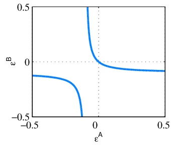
In this equation we have kept the leading non-trivial infinitesimal changes, discarding those of the type $(\epsilon^{{\hskip 0.85358pt\mbox{\tiny$\mathsf{A}$}}})^{2}$ and $(\epsilon^{{\hskip 0.85358pt\mbox{\tiny$\mathsf{B}$}}})^{2}$. This is the correct expansion in the space of jets of regular functions of two vectors with nonvanishing gradients. Equation (28) defines a surface similar to an hyperboloid. In order to visualize it one can simply take ${\epsilon_{i}^{{\hskip 0.85358pt\mbox{\tiny$\mathsf{A}$}},{\hskip 0.85358pt\mbox{\tiny$\mathsf{B}$}}}}=\delta_{1i}\epsilon^{{\hskip 0.85358pt\mbox{\tiny$\mathsf{A}$}},{\hskip 0.85358pt\mbox{\tiny$\mathsf{B}$}}}$. For a simple choice of $\alpha,\beta$, the result is plotted in figure 1. Clearly, connection to the identity implies that only the branch containing the origin has to be considered.

Therefore, the vectors $\epsilon^{{\hskip 0.85358pt\mbox{\tiny$\mathsf{A}$}},{\hskip 0.85358pt\mbox{\tiny$\mathsf{B}$}}}$ are constrained while the matrices $\phi^{{\hskip 0.85358pt\mbox{\tiny$\mathsf{A}$}},{\hskip 0.85358pt\mbox{\tiny$\mathsf{B}$}}}$ are unconstrained.²² 2 We are neglecting here the case $\alpha_{i}^{{\hskip 0.85358pt\mbox{\tiny$\mathsf{A}$}},{\hskip 0.85358pt\mbox{\tiny$\mathsf{B}$}}}=0$, $\beta_{ij}\neq 0$. In this atypical case we need to keep terms of ${\cal O}\left(\epsilon^{2}\right)$ in the transformation law of ${\hat{\mathbb{I}}}^{{\hskip 0.85358pt\mbox{\tiny$\mathsf{A}$}},{\hskip 0.85358pt\mbox{\tiny$\mathsf{B}$}}}$. Once this is done one checks that the codimension is still one. The really degenerate case $\alpha=\beta=0$, instead, corresponds to the class of equivalence of a single point ${\hat{\rho}}={\hat{\mathbb{I}}}^{\hskip 0.85358pt\mbox{\tiny$\mathsf{A}$}}\otimes{\hat{\mathbb{I}}}^{\hskip 0.85358pt\mbox{\tiny$\mathsf{B}$}}/{\mathsf{d}}$, with dimension 0. This point has to be considered as the ‘tip’, the extremal point of the space of states. Assuming that the SC’s are all different (i.e. that ${\hat{\rho}}$ is a ‘typical state’), one finds out that the Schmidt equivalence class $\mathfrak{S}_{\hat{\rho}}$ is locally diffeomorphic to

where the subgroup $\mathrm{SO}(2)$ is generated by the linear combination of the coefficients $\{\epsilon_{i}^{\hskip 0.85358pt\mbox{\tiny$\mathsf{A}$}},\epsilon_{i}^{\hskip 0.85358pt\mbox{\tiny$\mathsf{B}$}}\}_{i=1}^{{\mathsf{d}}-1}$ derived above. Then, the dimension of the manifold $\mathfrak{S}_{\hat{\rho}}$ is

It is easy to see how this counting is consistent with the intuition that changing one of the SC’s $\lambda_{1},\ldots,\lambda_{{\mathsf{d}}}$ of ${\hat{\rho}}$ brings out of the equivalence class $\mathfrak{S}_{\hat{\rho}}$. Indeed, subtracting the number of the SC’s from the number of dimensions — $({\mathsf{d}}^{2}-1)-{\mathsf{d}}={\mathsf{d}}^{2}-{\mathsf{d}}-1$ — we obtain the dimensionality of a typical orbit. For example, take the case of two-qubits: ${N_{\mbox{\tiny$\mathsf{A}$}}}={N_{\mbox{\tiny$\mathsf{B}$}}}=2$. We have: ${\mathsf{d}}=4$ and ${\mathsf{d}}^{2}-1=15$; hence, the manifold $\mathfrak{S}_{\hat{\rho}}$, for a typical bipartite state ${\hat{\rho}}\in\mathcal{D}(\mathcal{H})$, is $(15-4=11)$-dimensional.

If ${\hat{\rho}}\in\mathcal{D}(\mathcal{H})$ is a non-typical state, the dimension of the manifold $\mathfrak{S}_{\hat{\rho}}$ is smaller than ${\mathsf{d}}^{2}-{\mathsf{d}}-1$. In fact, in the case where the ${\mathsf{d}}$ SC’s of ${\hat{\rho}}$ cluster into subsets of $m_{1},...,m_{h}$ identical values — by means of an argument analogous to the one adopted in [24] — one can check that there is a ‘local stabilizer subgroup’ isomorphic to $\mathrm{SO}(m_{1})\times\dots\times\mathrm{SO}(m_{h})$; therefore, in this case, $\mathfrak{S}_{\hat{\rho}}$ is locally diffeomorphic to

Then, the dimension $\mathrm{d}_{{\hat{\rho}}}$ of $\mathfrak{S}_{\hat{\rho}}$ is given, in general, by

In order to make the above argument rigorous, one should actually prove that the Schmidt equivalence classes are actually differentiable manifolds. In that case our previous argument would provide the correct dimension of such manifolds. As we learn from mathematicians [25], a standard tool for characterizing a subset of a differentiable manifold (like the manifold of Hermitian operators in $\mathcal{H}$) as a submanifold is the study of the (possible) Lie groups acting transitively on the given subset and of the associated stabilizer subgroups. Therefore, suitably improving the analysis of subsection 3.1 may allow to achieve such a remarkable result.

References

• [1] Einstein A, Podolsky B, Rosen N 1935 Phys. Rev. 47 777
• [2] Schrödinger E 1935 Naturwissenschaften 23 807, 823, 844
• [3] Schrödinger E 1935 Proc. Camb. Phil. Soc. 31 555; 1936 ibid. 32 446
• [4] Nielsen M A, Chuang I L 2000, Quantum Computation and Quantum Information (Cambridge: Cambridge University Press)
• [5] Bouwmeester D, Ekert A and Zeilinger A (Eds.) 2000, The Physics of Quantum Information: Quantum Cryptography, Quantum Teleportation and Quantum Computation (New York: Springer)
• [6] Werner R F 1989 Phys. Rev.A 40 4277
• [7] Horodecki P 1997 Phys. Lett.A 233 333
• [8] Horodecki M, Horodecki P and Horodecki R 1996 Phys. Lett.A 223 1; Peres A 1996 Phys. Rev. Lett. 77 1413
• [9] Horodecki M, Horodecki P and Horodecki R 2006 Open Sys. Inf. Dyn. 13 103
• [10] Horodecki M, Horodecki P 1999 Phys. Rev.A 59 4206; Cerf N J, Adami C, Gingrich R M 1999 ibid. 60 898
• [11] Nielsen M A, Kempe J 2001 Phys. Rev. Lett. 86 5184
• [12] Chen K, Wu L A 2003 Quant. Inf. Comp. 3 193
• [13] Rudolph O 2002 Further results on the cross norm criterion for separability Preprint quant-ph/0202121; 2005 Quantum Information Processing 4 219
• [14] Sudarshan E C G, Mathews P M and Rau J 1961 Phys. Rev. 121 920
• [15] Jamiołkowski A 1972 Rep. Math. Phys. 3, 275
• [16] Ẑyczkowski K and Bengtsson I 2004 Open Sys. Inf. Dyn. 11 3
• [17] Holevo A S 1998 Coding Theorem for Quantum Channels Preprint quant-ph/9809023
• [18] Peres A 1993 Quantum Theory: Concepts and Methods (Dordrecht: Kluwer Academic Publishers)
• [19] Aniello P, Lupo C 2007 A new class of separability criteria for bipartite quantum systems Preprint quant-ph/0711.3390; to appear on J. Phys. A: Math. Gen.
• [20] Yu S and Liu N 2005 Phys. Rev. Lett. 95 150504
• [21] Gühne O and Lütkenhaus N 2006 Phys. Rev. Lett. 96 170502; Gühne O, Mechler M, Tóth G and Adam P 2006 Phys. Rev.A 74 010301(R); Zhang C J, Zhang Y S, Zhang S and Guo G C 2007 ibid. 76 012334; Zhang C J, Zhang Y S, Zhang S and Guo G C 2007 ibid. 77 060301(R)
• [22] Vidal G 2000 J. Mod. Opt. 47 355
• [23] Kadison R 1951 Annals of Mathematics 54, 325
• [24] Sinołȩcka M M, Ẑyczkowski K, Kuś M 2002 Act. Phys. Pol. B 33 2081
• [25] Varadarajan V S 1984 Lie Groups, Lie Algebras and Their Representations (New York: Springer-Verlag)
• [26] Horodecki M, Shor P W, Ruskai M B 2003 Rev. Math. Phys. 15 629; Ruskai M B 2003 ibid. 15 643
• [27] Wolf M M, Cirac J I 2008 Commun. Math. Phys. 279 147
• [28] Rudolph O 2003 Phys. Rev.A 67 032312