Self-energy renormalization around the flux phase in the $t-J$ model: Possible implications in underdoped cuprates

The pseudogap (PG) phase of high-$T_{c}$ cuprates presents unusual properties in clear contrast to those expected for conventional metals[1] and, in spite of the many scenarios proposed, the problem remains open. A well known phenomenological theory is the $d$-CDW[2] in which a normal state (NS) gap was proposed. Interestingly, $d$-CDW is closely related to the flux phase (FP) which was formerly predicted in the context of the $t-J$ model.[3] In both scenarios the PG coexists and competes with superconductivity, is complex and shows $d$-wave symmetry. FP was also studied by means of different analytical and numerical methods.[4, 5, 6, 7] In the mean field approximation of the $t-J$ model, below a characteristic temperature $T^{*}$, a $d$-wave NS gap opens on the Fermi surface (FS) near the hot spots (${\bf k}\cong(0,\pi)$). This leads to pockets with low spectral weight intensity in the outer section.[8] Thus, these pockets resemble the arcs observed in ARPES experiments.[9] Furthermore, recent progress on the $t-J$ model shows that the competition between FP and superconductivity leads to a phase diagram qualitatively similar to that observed in cuprates.[5] Raman and tunneling spectroscopy results show similarities with the experiment.[10] Very recent ARPES,[11] Raman,[12] specific heat,[13] and femtosecond optical pulses[14] experiments together with some theoretical developments[15] support the competing two-gap scenario. From the above reasons FP may be considered as a good candidate for describing the PG region. Nevertheless there are some drawbacks to be addressed. While in the FP scenario a true phase transition occurs at $T^{*}$, many experiments show a smooth behavior as a function of temperature.[16] In addition, well defined quasiparticle (QP) peaks are predicted everywhere on the Brilloiun zone (BZ), above and below $T^{*}$, while experiments show that the QP exists only near nodal direction.[17] Near hot spots, coherent peaks are observed neither below nor above the PG temperature in apparent contradiction with the FP picture. On the other hand, the PG observed in ARPES, consistently with tunneling experiments,[18] seems to be filling up but is not closing, [19] leading to a smooth evolution of spectral properties.

In spite of the above objections we will assume the point of view that the basic physics of cuprates is contained in the $t-J$ model (see Ref.[20] for discussions). Moreover, to address the above discussion it is necessary to perform a controllable self-energy and spectral function calculation beyond mean field. Recently it was proposed a large-$N$ approach for the $t-J$ model based on the path integral representation for $X$-operators.[6] At mean field level the approach of Ref.[6] agrees with slave boson[3, 4] and the approach of Ref.[5]. Additionally, it can be easily applied beyond mean field allowing the calculation of self-energy and spectral functions.[21] In this paper we discuss spectral functions and self-energy calculations in the NS in the vicinity to the FP instability. We have found that the spectral functions and the corresponding self-energies are very anisotropic on the FS leading to well defined QP near nodal direction and very incoherent features near hot spots.

We study the two dimensional $t-J$ model with hopping $t$ and Heisenberg coupling $J/t=0.3$ between nearest neighbors sites on the square lattice.[22] In the following energy is in units of $t$. Using the formulation described in Ref.[6] the mean field homogeneous Fermi liquid (HFL) becomes unstable when the static ($\omega=0$) flux susceptibility $\chi_{flux}({\bf q},\omega)=(\frac{\delta}{2})^{2}[(8/J)\Delta^{2}-\Pi({\bf q},\omega)]^{-1}$ diverges. $\Pi({\bf q},\omega)$ is an electronic bubble calculated with a form factor $\gamma({\bf q},{\bf k})=2\Delta(sin(k_{x}-q_{x}/2)-sin(k_{y}-q_{y}/2))$.[6, 21, 23] (For definition of $\Delta$ see below). In Fig.1a the phase diagram in the doping-temperature ($\delta-T$) plane is presented where $T^{*}$ indicates the FP instability onset. At $T=0$ a phase transition occurs at the critical doping $\delta_{c}\cong 0.12$ for the incommensurate critical vector ${\bf q}_{c}\cong(1,0.86)\pi$ near $(\pi,\pi)$. At finite $T$ the instability is commensurate (${\bf q}_{c}=(\pi,\pi)$). Therefore, since the instability takes place at, or close to, $(\pi,\pi)$ the form factor $\gamma({\bf q},{\bf k})$ transforms into $\sim(cos(k_{x})-cos(k_{y}))$ which indicates the $d$-wave character of the FP. Since $T^{*}$ falls abruptly to zero at $\delta_{c}$,[24] we associate the FP with the scenario discussed in Fig.1a of Ref.[16]. In Fig.1b we have plotted $Im\chi_{flux}({\bf q}=(\pi,\pi),\omega)$ at $T=0$ which shows that when $\delta\rightarrow\delta_{c}$ a low energy $d$-wave flux mode becomes soft accumulating large spectral weight. This soft mode reaches $\omega=0$ at $\delta=\delta_{c}$ freezing the FP.

In Fig.1c we have plotted the QP weight $Z=1/(1-\partial Re\Sigma/\partial\omega)$ vs $\delta$ for each self-energy contribution. $Z_{R\lambda}$ (black circles) are results at the Fermi crossing momentum in the $(0,0)$-$(0,\pi)$ direction (antinodal-$k_{F}$). $Z_{R\lambda}$ decreases (linearly) with decreasing doping ($Z_{R\lambda}\rightarrow 0$ when $\delta\rightarrow 0$). Due to the fact that $\Sigma_{R\lambda}$ is very isotropic on the FS, results for $Z_{R\lambda}$ at the Fermi crossing momentum in the nodal direction (nodal-$k_{F}$) are very similar to those for the antinodal-$k_{F}$. In contrast, $Z_{flux}$ (red squares) is strongly anisotropic on the FS. For nodal-$k_{F}$ (open red squares) $Z_{flux}\sim 1$ which means that $\Sigma_{flux}$ has no important contribution near nodal direction. For antinodal-$k_{F}$ (closed red squares) $Z_{flux}$ is rapidly decreasing with doping, i.e., $Z_{flux}\rightarrow 0$ when $\delta\rightarrow\delta_{c}$ where the flux instability takes place. In order to show explicitly the anisotropy of $\Sigma_{flux}$, in Fig.1d we have plotted $Z_{flux}$ versus the FS angle $\phi$ from $\phi=0$ (antinodal-$k_{F}$) to $\phi=\pi/4$ (nodal-$k_{F}$), for $\delta=0.13$. The soft $d$-wave mode (Fig.1b), which scatters electrons on the FS with momentum transfer ${\bf q}\sim(\pi,\pi)$, is responsible for the observed anisotropy. Using $Z_{R\lambda}$ and $Z_{flux}$ the total QP weight can be written as $Z_{T}=1/(Z_{R\lambda}^{-1}+Z_{flux}^{-1}-1)$. Blue triangles are the results for $Z_{T}$ at the antinodal-$k_{F}$. While for large $\delta$ self-energy renormalizations are dominated by $\Sigma_{R\lambda}$, $\Sigma_{flux}$ dominates near $\delta_{c}$. Results for $Z_{T}$ at the nodal-$k_{F}$ (not shown) follow the same trend as $Z_{R\lambda}$, i.e., the nodal $Z_{T}$ exhibits a linear behavior with slope similar to that discussed in Ref.[26].

Next we will consider the $\Sigma_{flux}$ contribution to the spectral function $A_{flux}({\bf k},\omega)$. Spectral functions for different $\delta$ values near $\delta_{c}$ at the antinodal-$k_{F}$ are presented for $T=0$ in Fig.2a. When $\delta\rightarrow\delta_{c}$, the area under the QP peak decreases (consistently with the behavior of $Z_{flux}$) and spectral weight is transfered to the incoherent structure at about $\omega\sim 0.05-0.1t$. Fig.2b shows the $\omega$ behavior of the flux scattering rate $Im\Sigma_{flux}$ at the antinodal-$k_{F}$ for several $\delta$ values near $\delta_{c}$. With decreasing doping towards $\delta_{c}$, $Im\Sigma_{flux}$ evolves from a FL-like behavior ($\sim\omega^{2}$) (see solid line for $\delta=0.20$) to a non FL-like behavior ($\sim\omega$) (see double-dotted-dashed line for $\delta=0.13$). At the same time, the structures (marked with arrows) that appear at low energy are correlated with the soft mode discussed in Fig.1b. $Im\Sigma_{flux}$ at the nodal-$k_{F}$ (not shown) is weaker than for the antinodal-$k_{F}$ and, in addition, it shows a FL-like behavior for all $\delta$ values. In summary, as observed in experiments, [27, 28] at low doping the scattering rate is strongly anisotropic on the FS presenting a FL-like ($\sim\omega^{2}$) behavior near the nodal-$k_{F}$ and a non FL-like ($\sim\omega$) behavior near the antinodal-$k_{F}$. In addition, this anisotropy disappears with overdoping where the behavior is more FL-like.

In Figs.2c and 2d spectral functions at the antinodal-$k_{F}$ are presented for $T=0.025$ and $T=0.035$, respectively. For a given temperature the intensity at the FS increases with increasing doping showing, consistently with experiments,[27, 17] a more clearly defined QP peak with overdoping. It is also interesting the following behavior. For instance, for $T=0.035$, with decreasing doping while the peak at the Fermi level loses intensity a broad shoulder appears at positive $\omega$ together with an apparent gap-like (which is not true gap) structure. As suggested by ARPES experiments,[19, 9] with increasing temperature the gap-like features seem to be filling up but are not closing (see results for $\delta=0.10$). Notice that for $\delta=0.10$ the leading edge below the FS is at $\omega=-0.05t$ which, using $t=0.4eV$, is about $20-30meV$ thus, of the order of the observed PG value.[19] Therefore, spectral functions are strongly temperature dependent, even at temperatures much lower than the hopping $t$, showing broad features at the antinodal-$k_{F}$. Spectral functions are nearly doping and temperature independent at the nodal-$k_{F}$ and show well defined QP peaks as in experiments.[27, 17] As mentioned above, at mean field level when the temperature decreases a gap opens at $T^{*}$ near hot spots. However, beyond mean field, spectral functions are very incoherent above $T^{*}$ showing that features expected to occur for $T<T^{*}$ already appear for $T>T^{*}$ due to self-energy renormalizations. For instance, the coherence loss when going from nodal-$k_{F}$ to antinodal-$k_{F}$ may suggest the appearance of arcs. Therefore, we think that self-energy corrections could be masking a likely abrupt change at $T^{*}$ given the appearance, in agreement with observations, of a smooth crossover. In addition, it may probably be that $T^{*}$ determined from the ARPES line-shape is somewhat shifted from the temperature at which PG opens.

The above results are due to the doping and temperature behavior of the self-energy. In Fig.2e we present results for $Im\Sigma_{flux}$ at $T=0.015$ for several $\delta$ values at the antinodal-$k_{F}$. While for $\delta=0.20$ $Im\Sigma_{flux}$ shows, as expected for a FL, the maximum at the Fermi level, with decreasing doping (see for instance double-dotted-dashed line for $\delta=0.13$) the maximum is shifted respect to $\omega=0$. As discussed in Refs.[29, 30], this behavior can damage the quasiparticle FL picture. For nodal-$k_{F}$ the situation is FL-like, e.g., $Im\Sigma_{flux}$ shows, for all doping values, the maximum at $\omega=0$ which increases with $T$ as $\sim T^{2}$. Notice the similarities between our self-energy results in Fig.2e and those discussed in Ref.[30].

In Fig.3 the $\omega=0$ spectral function intensity at the antinodal-$k_{F}$ is presented in the $\delta$-$T$ plane. The spectral intensity distribution suggests a crossover from a strange metal at low doping and high temperature to a FL at high doping and low temperature. Based on different arguments, recent works have proposed a similar picture. [31]

Before closing let us discuss the influence of $\Sigma_{R\lambda}$ on previous results. In Fig.4a self-energy results for $\Sigma_{R\lambda}$, $\Sigma_{flux}$ and $\Sigma_{T}$, at the antinodal-$k_{F}$, are presented for $\delta=0.13$ and $T=0.02$. $Im\Sigma_{R\lambda}$ (solid line) shows a FL-like behavior near $\omega=0$. The dotted-dashed line is the result for $Im\Sigma_{T}$ (eq.(1)). While at large frequency $\Sigma_{T}$ is dominated by $\Sigma_{R\lambda}$, properties near the FS are dominated by $\Sigma_{flux}$. $Im\Sigma_{T}$ at the nodal-$k_{F}$ is very similar to $Im\Sigma_{R\lambda}$ (solid line) because $\Sigma_{flux}$ has not important influence in the nodal direction. In Fig.4b, using $\Sigma_{T}$, the total spectral functions at the nodal-$k_{F}$ (solid line) and at the antinodal-$k_{F}$ (dashed line) are presented for low $\omega$. For the spectral function behavior at large $\omega$ see Ref.[21]. Although $\Sigma_{R\lambda}$ might modify our previous results, it remains the main tendency arising from $\Sigma_{flux}$, i.e., the spectral functions are strongly anisotropic on the FS, losing intensity and becoming broad when going from nodal-$k_{F}$ to antinodal-$k_{F}$.

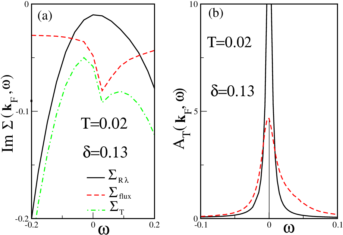
Concluding, in the framework of the $t-J$ model we have computed self-energy corrections in the vicinity of the FP instability. The corresponding spectral functions are anisotropic on the FS and very incoherent near hot spots thus, they show features similar to those observed in experiments. In agreement with recent discussions (see Ref.[28] and references their in) our results show two contributions to the scattering channel. One contribution ($\Sigma_{flux}$) is strongly anisotropic on the FS, the other one ($\Sigma_{R\lambda}$) is very isotropic. $\Sigma_{flux}$ dominates at low doping (near $\delta_{c}$) and low energy being relevant for the PG properties. In contrast, $\Sigma_{R\lambda}$ dominates at large doping and large $\omega$. In Ref.[32], by means of transport measurements, it was found that an isotropic scattering channel dominates in overdoped samples which agrees with our predictions for $\Sigma_{R\lambda}$. In a recent work[33] it was proposed that the high energy features observed in ARPES[34] may be due to the large $\omega$ behavior of $\Sigma_{R\lambda}$. Finally, our results indicate that some problems, which can be interpreted against the FP scenario, may be less serious after including self-energy renormalizations.

The author thanks to M. Bejas, A. Foussats, H. Parent, A. Muramatsu, and R. Zeyher for valuable discussions.

References

- [1] T. Timusk and B. Statt, Rep. Prog. Phys. 62, 61 (1999).
- [2] S. Chakravarty, R. B. Laughlin, D. K. Morr, and C. Nayak, Phys. Rev. B 63, 094503 (2001).
- [3] I. Affleck and J. B. Marston, Phys. Rev. B 37, 3774 (1988). T. C. Hsu, B. J. Marston, and I. Affleck, Phys. Rev. B 43, 28661 (1988)
- [4] D. C. Morse and T. C. Lubensky, Phys. Rev. B 42, 7994 (1990).
- [5] E. Cappelluti and R. Zeyher, Phys. Rev. B 59, 6475 (1999).
- [6] A. Foussats and A. Greco, Phys. Rev. B 70, 205123 (2004).
- [7] P. W. Leung, Phys. Rev. B 43, 6612 (R) (2000).
- [8] S. Chakravarty, C. Nayak, and S. Tewari, Phys. Rev. B 68, 100504 (R) (2003).
- [9] M. R. Norman, H. Ding, M. Randeria, J. C. Campuzano, T. Yokoya, T. Takeuchi, T. Takahashi, T. Mochiku, K. Kadowaki, P. Guptasarma, D. G. Hinks, Nature 392, 157 (1998).
- [10] R. Zeyher and A. Greco, Phys. Rev. Lett. 89, 177004 (2002). A. Greco and R. Zeyher, Phys. Rev. B 70, 024518 (2004).
- [11] T. Kondo, Tsunehiro Takeuchi, Adam Kaminski, Syunsuke Tsuda, and Shik Shin, Phys. Rev. Lett. 98, 267004 (2007). M. Hashimoto, T. Yoshida, K. Tanaka, A. Fujimori, M. Okusawa, S. Wakimoto, K. Yamada, T. Kakeshita, H. Eisaki, and S. Uchida, Phys. Rev. B 75, 140503 (R) (2007).
- [12] M. Le Tacon, A. Sacuto, Y. Gallais, D. Colson, and A. Forget, Phys. Rev. B 76, 144505 (2007).
- [13] H.-H. Wen and X.-G. Wen, Physica C 460, 28 (2007).
- [14] Elbert E. M. Chia, Jian-Xin Zhu, D. Talbayev, R. D. Averitt, and A. J. Taylor, Phys. Rev. Lett. 99, 147008 (2007).
- [15] B. Valenzuela and E. Bascones, Phys. Rev. Lett. 98, 227002 (2007). T. Das, R. S. Markiewicz, and A. Bansil, arXiv:0711.0480.
- [16] J. L. Tallon and J. W. Loran, Physica C 349, 53 (2001).
- [17] C. Kim, P. J. White, Z.-X. Shen, T. Tohyama, Y. Shibata, S. Maekawa, B. O. Wells, Y. J. Kim, R. J. Birgeneau, and M. A. Kastner, Phys. Rev. Lett. 80, 4245 (1998).
- [18] Ch. Renner, B. Revaz, J.-Y. Genoud, K. Kadowaki, and Ø. Fischer, Phys. Rev. Lett. 80, 149 (1998).
- [19] C. Norman, M. Randeria, H. Ding, and J. C. Campuzano, Phys. Rev. B 57, 11093 (R) (1998).
- [20] P. Lee, N. Nagaosa, and X.-G. Wen, Rev. Mod. Phys. 78, 17 (2006).
- [21] M. Bejas, A. Greco, and A. Foussats, Phys. Rev. B 73, 245104 (2006).
- [22] For simplicity and without losing generality we have considered the minimal model. The inclusion of hopping between second, third, etc neighbors sites produces only small quantitative but not qualitative changes.
- [23] This form factor is obtained after projecting the electron-boson vertex (eq.(9) in Ref.[6]) on the corresponding eigenvector for the FP instability.
- [24] The inclusion of a hopping between second neighbors simply shifts to values closer to the experimental[16] (see Ref.[10]).
- [25] is the fluctuation of the charge Hubbard operator () associated to the number of holes. is the fluctuation of the Lagrangian multiplier related to the nondouble occupancy constraint .
- [26] T. Yoshida, X. J. Zhou, T. Sasagawa, W. L. Yang, P. V. Bogdanov, A. Lanzara, Z. Hussain, T. Mizokawa, A. Fujimori, H. Eisaki, Z.-X. Shen, T. Kakeshita, and S. Uchida, Phys. Rev. Lett. 91, 027001 (2003).
- [27] A. Kaminski, H. M. Fretwell, M. R. Norman, M. Randeria, S. Rosenkranz, U. Chatterjee, J. C. Campuzano, J. Mesot, T. Sato, T. Takahashi, T. Terashima, M. Takano, K. Kadowaki, Z. Z. Li, and H. Raffy, Phys. Rev. B 71, 014517 (2005).
- [28] J. Chang, M. Shi, S. Pailhes, M. Maansson, T. Claesson, O. Tjernberg, A. Bendounan, L. Patthey, N. Momono, M. Oda, M. Ido, C. Mudry, J. Mesot, arXiv:0708.2782.
- [29] A. A. Katanin and A. P. Kampf, Phys. Rev. Lett. 93, 106406 (2004).
- [30] L. Dell’Anna and W. Metzner, Phys. Rev. B 73, 045127 (2006).
- [31] H. Castro and G. Deutscher, Phys. Rev. B 70, 174511 (2004). A. Kaminski, S. Rosenkranz, H. M. Fretwell, Z. Z. Li, H. Raffy, M. Randeria, M. R. Norman, and J. C. Campuzano, Phys. Rev. Lett. 90, 207003 (2003).
- [32] S. Nakamae, K. Behnia, N. Mangkorntong, M. Nohara, H. Takagi, S. J. C. Yates, and N. E. Hussey, Phys. Rev. B 68, 100502 (R) (2003).
- [33] A. Greco, Solid State Communications 142, 318 (2007).
- [34] B. Xie, K. Yang, D. W. Shen, J. F. Zhao, H. W. Ou, J. Wei, S. Y. Gu, M. Arita, S. Qiao, H. Namatame, M. Taniguchi, N. Kaneko, H. Eisaki, K. D. Tsuei, C. M. Cheng, I. Vobornik, J. Fujii,5 G. Rossi, Z. Q. Yang, and D. L. Feng Phys. Rev. Lett. 98, 147001 (2007). Z.-H. Pan, P. Richard, A.V. Fedorov, T. Kondo, T. Takeuchi, S.L. Li, Pengcheng Dai, G.D. Gu, W. Ku, Z. Wang, H. Ding cond-mat/0610442.