Geometric Scaling from DGLAP evolution

The observation of geometric scaling [1] in $ep$ deep inelastic scattering (DIS) data has attracted considerable interest because it is widely interpreted as evidence for parton recombination and saturation [2]. Geometric scaling (GS) is the statement that the total $\gamma^{*}p$ cross section $\sigma_{tot}^{\gamma^{*}p}$, which is a priori function of two independent variables — the photon virtuality $Q^{2}$ and the Bjorken variable $x$ — only depends on the variable $\tau=Q^{2}/Q_{s}^{2}(x)$, where the so–called saturation scale $Q_{s}^{2}(x)$ depends nontrivially on $x$, with dimensions given by a fixed reference scale $Q_{0}^{2}$.

The presence of recombination effects in the HERA data would have dramatic effects, because these data dominate the determination of parton distributions, which are necessary for the computation of LHC processes [3]. Available parton fits do not include these effects and would thus fail to provide reliable predictions at the LHC. It is the purpose of this paper to ascertain whether this is actually the case, and more in general, in which kinematic region GS may or may not provide evidence for saturation.

Evidence for GS is provided by the scaling plot of the reduced cross section $\sigma_{tot}^{\gamma^{*}p}$ vs. the scaling variable $\tau$:

where $t=\ln Q^{2}/Q_{0}^{2}$, and the saturation scale $t_{s}\equiv\ln\frac{Q^{2}_{s}(x)}{Q_{0}^{2}}$ was originally [1] chosen as $t_{s}=\lambda\xi$, and more recently [2, 4] also as $t_{s}=\lambda\sqrt{\xi}$, with $\xi=\ln(1/x)$. To test whether this behaviour is compatible with standard DGLAP perturbative evolution, in Figs. 2-3 we show a scaling plot of $\sigma_{tot}^{\gamma^{*}p}$ computed using the double asymptotic scaling (DAS) approximation to leading–order (LO) DGLAP evolution [5] of a constant boundary condition. Namely, we take

where $\sigma\equiv\sqrt{\xi\ln\frac{t+\bar{t}_{0}}{\bar{t}_{0}}}$, $\rho\equiv\sqrt{\xi/\ln\frac{t+\bar{t}_{0}}{\bar{t}_{0}}}$, $\bar{t}_{0}\equiv\ln\frac{Q_{0}^{2}}{\Lambda_{QCD}^{2}}$ and $\beta_{0}=11-\frac{2}{3}n_{f}$, $\gamma=\sqrt{\frac{12}{\beta_{0}}}$.

The DAS approximation to LO DGLAP evolution is quite accurate in a wide kinematic region $Q^{2}\mathrel{\hbox to0.0pt{\raise 2.20013pt\hbox{$>$}\hss}{\lower 2.20013pt\hbox{$\sim$}}}10$ GeV², $x\mathrel{\hbox to0.0pt{\raise 2.20013pt\hbox{$<$}\hss}{\lower 2.20013pt\hbox{$\sim$}}}0.1$, based on approximating the LO anomalous dimension as

We take it as representative of a situation where saturation is certainly absent. The GS properties of the cross section Eq. (2) are compared to those of the data by plotting both vs. $\tau$, with the best–fit phenomenological values of Ref. [4] $\lambda=0.321$ (Fig. 2) or $\lambda=1.621$ (Fig. 3), over the grid of $(x,Q^{2})$ values shown in Fig. 1. The data points are obtained from a very accurate neural network interpolation to world DIS data [6]. The kinematical region is that for which experimental data are available.

Figs. 2-3 show that for $\tau\mathrel{\hbox to0.0pt{\raise 2.20013pt\hbox{$>$}\hss}{\lower 2.20013pt\hbox{$\sim$}}}1$ (Fig. 2) or $\tau\mathrel{\hbox to0.0pt{\raise 2.20013pt\hbox{$>$}\hss}{\lower 2.20013pt\hbox{$\sim$}}}0.1$ (Fig. 3) the GS properties of the DAS solution are almost as good as those of the data, and become as good or better with a minor improvement, to be discussed below. It follows that saturation is by no means necessary for geometric scaling. This may seem surprizing given that the DAS solution Eq. (2) appears to violate GS. However, we now show that approximate GS is in fact a general property of solutions to the DGLAP equation. It is already known that if GS is imposed as a boundary condition at some low scale, it is preserved by both BFKL [2] or DGLAP [7] linear evolution to higher scales. Here, we show instead that GS is generated by linear DGLAP evolution itself, irrespective of the choice of boundary condition.

Consider first the fixed–coupling case. The general DGLAP solution for any anomalous dimension $\gamma$ is

where $G_{0}(N)$ is a suitable boundary condition. For large enough $\xi$, the integral can be evaluated in the saddle point approximation. The saddle condition is

The cross section becomes

up to terms which are not enhanced as $\xi\to\infty$.

Geometric scaling follows expanding $t$ about the saturation scale Eq. (1) $t_{s}=\lambda\xi$:

If we choose a value of $\lambda$ such that $f(\lambda)=0$ the cross section Eq. (8) manifestly displays geometric scaling. It is apparent from Eq. (7) that this value exists if $\gamma$ is the DGLAP anomalous dimension, either at fixed perturbative order or resummed at small $x$ using the BFKL formalism, or indeed for any reasonable shape of $\gamma$.

This argument is in fact quite close to that of Ref. [2], due to the fact that the DGLAP solution can equivalently be written in “dual” form [8] as

where the kernel $\chi$ is related to $\gamma$ by

and $\bar{G}_{0}(M)$ is determined in terms of the boundary condition $G_{0}(N)$ and the anomalous dimension $\gamma$. Evaluating the integral (9) by saddle point and then Taylor expanding reproduces the argument for geometric scaling of Ref. [2]. However, Eq. (8) shows that the “saturation” assumption of Refs. [2, 7] that the boundary condition satisfies GS is redundant: rather, GS follows from the existence of $\lambda$ such that $f(\lambda)=0$ in Eq. (8). This is a generic property of perturbative evolution. Equation (9) can be equivalently viewed as the solution to the BFKL or DGLAP equations, and our conclusion applies to both.

We conclude that GS holds for the solution to the DGLAP equation at the fixed coupling level, which explains the GS properties of the DAS solution Eq. (2), Fig. 2: this solution is derived with running coupling, but in practice (see Fig. 1), the value of $t$ along fixed $\tau$ curves is almost constant in the data region. It follows that $\frac{1}{\beta_{0}}\ln[(t+\bar{t}_{0})/\bar{t}_{0}]\approx\alpha_{s}(Q_{0}^{2})\,t$, which in turn implies that Eq. (3) holds with $\sigma\approx\sqrt{\xi\beta_{0}\alpha_{s}t}$ and $\rho\approx\sqrt{\xi/(\beta_{0}\alpha_{s}t)}$, which coincides with the result found using Eq. (4) in the approximation Eq. (7). Higher order terms in this expansion lead to GS violations, proportional to powers of $\alpha_{s}(Q_{0}^{2})t$. The combined effect of GS violations will be discussed in Fig. 4 below.

A running coupling form of GS can also be derived [9] directly for the cross section Eq. (2-3). At the running coupling level, we can neglect the variation of $\ln t/t_{0}$ in $\sigma$ and $\rho$ in comparison to the scale dependence of $Q^{-2}$ in Eq. (2). Then, the DAS solution (3) only depends on $\sqrt{\xi}$, and the cross section (2), consistently neglecting the variation of $\ln\xi$ in comparison to the variation of $\xi$, is a function of the scaling variable $t-\lambda\sqrt{\xi}$.

Note that, unlike the fixed coupling GS in terms of $t-\lambda\xi$, Eq. (8), which holds for a generic anomalous dimension $\gamma$, this running coupling GS depends on the particular form of the anomalous dimension Eq. (4), and specifically on the fact that it has a simple pole at $N=0$. However, this running coupling GS can also be obtained using the running–coupling version of Eq. (9)  [10, 11]

which holds whenever the kernel $\chi$ Eq. (10) is linear in $\alpha_{s}$. This is the case if we only retain the simple pole in the anomalous dimension $\gamma$ Eq. (4), but also for a generic leading–order BFKL kernel, as discussed in Ref. [12]. The argument leading to GS Eq. (8) can now be repeated: the only difference is that the saddle point depends on $t/\sqrt{\xi}$, which leads to the form $t_{s}=\lambda\sqrt{\xi}$ of the saturation scale.

The arguments so far involved several approximations. To assess their accuracy, we express the cross section as a function of $\ln\tau=t-\lambda\xi$ and the orthogonal combination $\zeta=t+\lambda\xi$. Geometric scaling is the statement that $\sigma_{tot}^{\gamma^{*}p}$ is independent of $\zeta$:

By letting $\lambda$ depend on $\xi$ and $t$, we can view the condition  (12) as an implicit equation for $\lambda(\xi,t)$. Geometric scaling holds to good approximation if the solution $\lambda(\xi,t)$ to Eq. (12) is approximately constant in $\xi$ and $t$ in the kinematic region of interest.

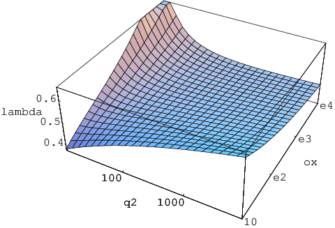
We see from Fig. 4 that the value of $\lambda$ is almost constant everywhere, except at low $Q^{2}\mathrel{\hbox to0.0pt{\raise 2.20013pt\hbox{$<$}\hss}{\lower 2.20013pt\hbox{$\sim$}}}25$ GeV². At low $Q^{2}$, large $x$ there are no data (see Fig. 1); while the low $Q^{2}$, low $x$ region, where the DAS solution is not applicable, shall be discussed below. We would now like to test whether instead in the region $Q^{2}\mathrel{\hbox to0.0pt{\raise 2.20013pt\hbox{$>$}\hss}{\lower 2.20013pt\hbox{$\sim$}}}25$ GeV² the approximate GS displayed in Fig. 4 is sufficient to explain the GS of the data. To this purpose, we use the “quality factor” $Q(\lambda)$ which was introduced in Ref. [4] as a measure of the scaling quality. The optimal value of $\lambda$ is that which maximizes $Q$, and GS is better if $Q(\lambda)$ is larger. In practice, the optimal value of $\lambda$ and the uncertainty on it are determined by fitting a gaussian form to $Q(\lambda)$. The values used to produce Figs. 2-3, taken from Ref. [4], were determined thus.

In Fig. 5 we display the quality factor $Q(\lambda)$, computed for all points with $Q^{2}>25$ GeV², both for the data and the DAS solution, as well as the result of a gaussian fit. We see that GS is actually rather better for the DAS solution than for the data. However, we also see that the optimal value of $\lambda$ for the DAS solution is somewhat larger. This explains why the GS properties of the DAS solution in Fig. 2 actually look a bit worse: the optimal value of $\lambda$ is not quite the same for the data and for the DAS solution.

To explain this difference, we note [13] that for medium-large $Q^{2}$ the DAS approximation can be substantially improved by including the contribution of the smaller eigenvector of the anomalous dimension matrix, whereby in Eq. (2) $F_{2}=(\gamma/\rho)G+\bar{G}$, where $\bar{G}(\xi,t)=k\exp(-\delta\sigma/\rho)$, with $\delta=16n_{f}/(27\beta_{0})$ and $k=0.16$ is determined from a fit to the data. The GS plot for this improved DAS solution is also shown in Fig. 2, and the corresponding quality factor is displayed in Fig. 5: GS deteriorates slightly for $Q^{2}>25$ GeV², but remarkably it now holds for all data of Fig. 2. Also, the optimal value of $\lambda$ extracted from the data and the improved DAS solution now agree. This means that linear leading–order perturbative evolution, as embodied by the (improved) DAS solution, can actually predict the optimal choice of saturation scale Eq. (1). Indeed, a gaussian fit to the quality factor for the improved DAS solution on all points of Fig. 2 ($Q^{2}>10$ GeV²) gives $\lambda=0.32\pm 0.05$, in perfect agreement with the value $\lambda=0.32\pm 0.06$ determined in Ref. [4] from the data. We take this as very strong evidence that GS for $Q^{2}\mathrel{\hbox to0.0pt{\raise 2.20013pt\hbox{$>$}\hss}{\lower 2.20013pt\hbox{$\sim$}}}10$ GeV² follows from purely linear perturbative arguments.

A similar analysis based on Eq. (12), but with the running coupling form of $\ln\tau=t-\lambda\sqrt{\xi}$ and $\zeta=t+\lambda\sqrt{\xi}$ leads to the same conclusion. In particular, in this case we predict $\lambda=1.66\pm 0.34$ to be compared to the experimental value $\lambda=1.62\pm 0.25$ of Ref. [4].

It remains to be understood why the data still display GS even at low $Q^{2}$ where the DAS solution becomes unrealiable. Figure 4 suggests that the effective value of $\lambda$ which characterizes perturbative evolution starts growing significantly for $Q^{2}\mathrel{\hbox to0.0pt{\raise 2.20013pt\hbox{$<$}\hss}{\lower 2.20013pt\hbox{$\sim$}}}10$ GeV². Because GS is nevertheless seen in this data region (see Fig. 2-3), one might conclude that there is some evidence for saturation there.

However, so far we have only used pure leading–order DGLAP evolution, which fails in this region because it does not resum small $x$ logarithms. Before concluding that a saturation-based approach is necessary, we should address the issue of small $x$ resummation in the framework of linear perturbative evolution. The small $x$ resummation of DGLAP evolution has been recently performed, based on a suitable matching of the BFKL and DGLAP solutions [14, 15]. For our present purpose, it is enough to consider the asymptotic small $x$ behaviour of these matched solutions, which is essentially determined [11, 14] by a quadratic approximation to a running–coupling BFKL evolution kernel.

As is well known [16], this leads to a solution written in terms of Airy functions $G_{A}(N,t)$ if the kernel is linear in $\alpha_{s}$ (Bateman functions [14] if the nonlinear dependence is retained). One can then extract [11] an anomalous dimension

The asymptotic small $x$ behaviour of DGLAP evolution at the resummed level is controlled by the rightmost singularity of $\gamma_{A}(\alpha_{s}(t),N)$ Eq. (13). This singularity turns out to be a simple pole, located at $N=N_{0}(t)$.

Neglecting the weak [11] scale dependence of $N_{0}$ the predicted asymptotic small $x$ behaviour at the resummed level is

This behaviour should hold in a region where $Q^{2}$ is large enough for some resummed linear perurbative evolution from a low–scale boundary condition to have taken place, say $5\mathrel{\hbox to0.0pt{\raise 2.20013pt\hbox{$<$}\hss}{\lower 2.20013pt\hbox{$\sim$}}}Q^{2}\mathrel{\hbox to0.0pt{\raise 2.20013pt\hbox{$<$}\hss}{\lower 2.20013pt\hbox{$\sim$}}}10$ GeV². In this region, we thus get GS with $\lambda=N_{0}$. Typical values of $N_{0}$ from resummed linear perturbative evolution are $0.1\mathrel{\hbox to0.0pt{\raise 2.20013pt\hbox{$<$}\hss}{\lower 2.20013pt\hbox{$\sim$}}}N_{0}\mathrel{\hbox to0.0pt{\raise 2.20013pt\hbox{$<$}\hss}{\lower 2.20013pt\hbox{$\sim$}}}0.3$ [14]. The GS properties of the unresummed DAS solution are thereby extended down to scales of order $5\mathrel{\hbox to0.0pt{\raise 2.20013pt\hbox{$<$}\hss}{\lower 2.20013pt\hbox{$\sim$}}}Q^{2}\mathrel{\hbox to0.0pt{\raise 2.20013pt\hbox{$<$}\hss}{\lower 2.20013pt\hbox{$\sim$}}}10$ GeV².

The scale dependence of $N_{0}$ can be kept into account by determining it in an expansion in powers of $\alpha_{s}^{2/3}(t)$ [11]

where $c=\frac{\chi^{q}(\alpha_{s},M_{0})}{\alpha_{s}}$ and $k=\frac{1}{2\alpha_{s}}\frac{\partial^{2}}{\partial M^{2}}\chi^{q}(\alpha_{s},M)|_{M=M_{0}}$ parametrize the quadratic BFKL kernel $\chi^{q}(\alpha_{s},M)$ at its minimum $M=M_{0}$.

Substituting this in Eq. (14) and expanding we see that the asymptotic form of the cross section is constant on the curve

This corresponds to the previously discussed running coupling form of the saturation scale, with $\lambda=\sqrt{\frac{4\pi c}{\beta_{0}}}$. Realistic [14] values $1\mathrel{\hbox to0.0pt{\raise 2.20013pt\hbox{$<$}\hss}{\lower 2.20013pt\hbox{$\sim$}}}c\mathrel{\hbox to0.0pt{\raise 2.20013pt\hbox{$<$}\hss}{\lower 2.20013pt\hbox{$\sim$}}}2$ give $1.2\mathrel{\hbox to0.0pt{\raise 2.20013pt\hbox{$<$}\hss}{\lower 2.20013pt\hbox{$\sim$}}}\lambda\mathrel{\hbox to0.0pt{\raise 2.20013pt\hbox{$<$}\hss}{\lower 2.20013pt\hbox{$\sim$}}}1.7$. This implies GS along this saturation line, and approximate GS in the proximity of it. Of course, if we go very far from this region we end up in the large $Q^{2}$ region which we have already discussed.

Hence, thanks to small $x$ resummation the growth Fig. 4 of $\lambda$ at small $x$ for $5\mathrel{\hbox to0.0pt{\raise 2.20013pt\hbox{$<$}\hss}{\lower 2.20013pt\hbox{$\sim$}}}Q^{2}\mathrel{\hbox to0.0pt{\raise 2.20013pt\hbox{$<$}\hss}{\lower 2.20013pt\hbox{$\sim$}}}10$ GeV² is replaced by the (almost) constant value $N_{0}$, thus extending GS to this region, with $t_{s}=N_{0}\xi$ or $t_{s}=\sqrt{4\pi c/\beta_{0}}\sqrt{\xi}$.

In conclusion, we have shown that for $Q^{2}\mathrel{\hbox to0.0pt{\raise 2.20013pt\hbox{$>$}\hss}{\lower 2.20013pt\hbox{$\sim$}}}10$ GeV² standard linear leading-order DGLAP perturbative evolution explains geometric scaling, and in fact predicts the value of the constant $\lambda$ which characterizes the “saturation” scale Eq. (1). Small $x$ resummation of the linear evolution equation extends the region where GS is expected to values of $Q^{2}$ which are lower, but still within the perturbative region. For yet lower values of $Q^{2}\mathrel{\hbox to0.0pt{\raise 2.20013pt\hbox{$<$}\hss}{\lower 2.20013pt\hbox{$\sim$}}}5$ GeV², geometric scaling, which is observed in the data, cannot be explained using linear perturbation theory. This is the region $\tau\mathrel{\hbox to0.0pt{\raise 2.20013pt\hbox{$<$}\hss}{\lower 2.20013pt\hbox{$\sim$}}}0.1$ (fixed-coupling $t_{s}$, Fig. 2) or $\tau\mathrel{\hbox to0.0pt{\raise 2.20013pt\hbox{$<$}\hss}{\lower 2.20013pt\hbox{$\sim$}}}0.01$ (running-coupling $t_{s}$, Fig. 3), where the GS plot flattens out. In this region, geometric scaling may provide genuine evidence for parton saturation.

Acknowledgements: We thank R. D. Ball and J. Rojo for a critical reading of the manuscript. This work was partly supported by the European network HEPTOOLS under contract MRTN-CT-2006-035505 and by a PRIN2006 grant (Italy).

References

- [1] A. M. Stasto, K. J. Golec-Biernat and J. Kwieciński, Phys. Rev. Lett. 86, 596 (2001).
- [2] See e.g. E. Iancu, K. Itakura and L. McLerran, Nucl. Phys. A 708 (2002) 327 and ref. therein.
- [3] M. Dittmar et al., arXiv:hep-ph/0511119.
- [4] F. Gelis, R. Peschanski, G. Soyez and L. Schoeffel, Phys. Lett. B 647, 376 (2007).
- [5] A. De Rujula et al., Phys. Rev. D 10, 1649 (1974); R. D. Ball and S. Forte, Phys. Lett. B 335, 77 (1994).
- [6] L. Del Debbio et al. [NNPDF Collaboration], JHEP 0503, 080 (2005).
- [7] J. Kwiecinski and A. M. Stasto, Phys. Rev. D 66, 014013 (2002).
- [8] T. Jaroszewicz, Phys. Lett. B 116, 291 (1982); R. D. Ball and S. Forte, Phys. Lett. B 405, 317 (1997); G. Altarelli, R. D. Ball and S. Forte, Nucl. Phys. B 575, 313 (2000).
- [9] E. Avsar and G. Gustafson, JHEP 0704, 067 (2007).
- [10] L. P. A. Haakman, O. V. Kancheli and J. H. Koch, Nucl. Phys. B 518, 275 (1998).
- [11] G. Altarelli, R. D. Ball and S. Forte, Nucl. Phys. B 621, 359 (2002).
- [12] S. Munier and R. Peschanski, Phys. Rev. D 69, 034008 (2004).
- [13] L. Mankiewicz, A. Saalfeld and T. Weigl, Phys. Lett. B 393, 175 (1997).
- [14] See G. Altarelli, R. D. Ball and S. Forte, arXiv:0802.0032 [hep-ph] and ref. therein.
- [15] See M. Ciafaloni, D. Colferai, G. P. Salam and A. M. Stasto, JHEP 0708, 046 (2007) and ref. therein.
- [16] L. N. Lipatov, Sov. Phys. JETP 63, 904 (1986).