The conjugacy problem in right-angled Artin groups and their subgroups

We start by recalling the following classical lemma.

Now we introduce our main tool, the notion of a piling.

The word associated with the generator $a_{i}$ will be called the $a_{i}$-stack of the abstract piling. The product of two abstract pilings is defined as the piling obtained by concatenation of the corresponding stacks.

We define a function $\pi^{\star}$ on the set $\{a_{1}^{\pm 1},\ldots,a_{N}^{\pm 1}\}^{*}$ of words on the $2n$ letters $a_{1},a_{1}^{-1},\ldots,a_{N},a_{N}^{-1}$ that associates an abstract piling to every word in the following way: starting with the empty piling, we read the word from left to right. When a letter $a_{i}^{\epsilon}$ is read, we check what the last letter of the $a_{i}$-stack of the piling is. If this letter is different from $-\epsilon$ (the no-cancellation cases: the $a_{i}$-stack is empty, or finishes either with $0$ or $\epsilon$), then we append a letter $+$ or $-$ at the end of the $a_{i}$-stack of the piling (the sign of $\epsilon$). Moreover, we also append a letter $0$ at the end of each of the $a_{j}$-stacks associated with a generator $a_{j}$ that does not commute with the generator $a_{i}$. On the other hand, if the last letter of the $a_{i}$-stack is $-\epsilon$ (the cancellation case), then we erase this last letter, and we also erase the terminal letter of each of the $a_{j}$-stacks of the piling associated with a generator $a_{j}$ that does not commute with the generator $a_{i}$ – note that the terminal letter of the $a_{j}$-stack is necessarily “$0$”.

We observe that the number of letters $+$ and $-$ occuring in the piling $\pi^{\star}(w)$ is at most equal to the length of the word $w$. Moreover, it is immediate from the description of the function $\pi^{\star}$ that, given a word $w$ of length $\ell$, the piling $\pi^{\star}(w)$ can be calculated in time $O(\ell)$ (linear-time).

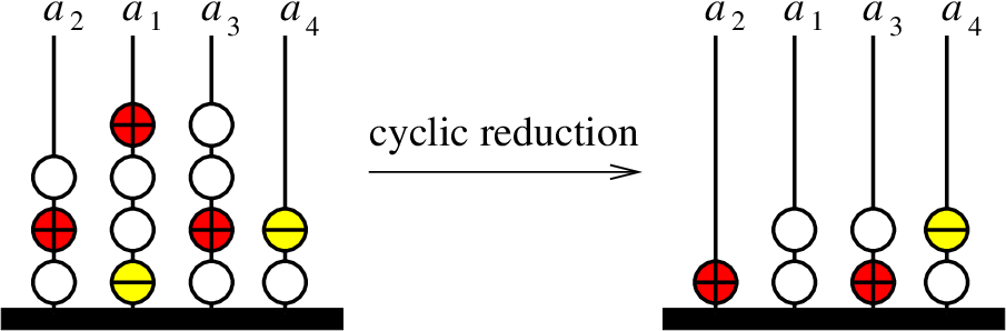
It may be helpful to keep in mind the following physical interpretation of a piling: we have $N$ vertical sticks, labelled by the generators $a_{1},\ldots,a_{n}$, with beads on it; the beads are labelled by $+$, $-$ or $0$ such that when reading from bottom to top the sequence of labels of the beads on the $a_{i}$-stick, we obtain the $a_{i}$-stack of the piling. A letter $a_{i}$ or $a_{i}^{-1}$ of the word $w$ corresponds to a set of beads (which we call a tile), consisting of one bead labelled $+$ or $-$ on the corresponding stick, and one bead labelled $0$ on each of the sticks corresponding to generators of $A$ which do not commute with $a_{i}$; each $0$ labelled bead is connected to the $\pm$ labelled bead by a thread. The rule is: on a stick, adjacent $0$-beads can commute with (“slide through”) each other, but $0$-beads do not commute with $\pm$-beads. In this physical model, we construct the image of a word by adding beads from the top, and removing opposed tiles when one obtains on a stick two adjacent $\pm$-beads with opposite signs. In fact, when we are dealing with the word problem we can forget about the threads between the beads, but they are helpful for thinking about the conjugacy problem.

The map $\pi^{\star}$ induces a well-defined function $\pi\colon\thinspace A\to\Pi$ because words representing the same element of $A$ have the same image under $\pi^{\star}$: the image of a word is unchanged by applying a commutation relation, and by inserting or deleting a trivial pair $a_{i}a_{i}^{-1}$ or $a_{i}^{-1}a_{i}$. Now, from the definitions it is immediate that no cancellation occurs during the construction of the piling $\pi^{\star}(w)$ of a reduced word $w$. Then, the identity of $A$ is the unique element of $A$ whose image by $\pi$ is the trivial piling, and therefore the word problem is solved in linear-time: a word $w$ represents the identity if and only if its piling $\pi^{\star}(w)$ is trivial; this piling can be built in linear-time.

The following notion will be extremely useful in the next section when we consider the conjugacy problem.

We remark that all the factors of a normal word are normal words.

We are now ready to attack the conjugacy problem.

The centralizer of a cyclically reduced element of $A$ has a canonical finite generating set: suppose that $w$ is a cyclically reduced word, written as a product of cyclically reduced non-split words $w=w_{1}\cdots w_{k}$, c.f. Section 2.2.2. Then, according to [6], for each $i$ in $\{1,\ldots,k\}$ there exists a unique maximal infinite-cyclic subgroup of $A$ containing $[w_{i}]$, generated by some cyclically reduced element $[z_{i}]$, and by [25] the centralizer of $[w]$ in $A$ is generated by

1. 1.

   the elements $[z_{i}]$, and

2. 2.

   the generators of $A$ which commute with all the generators occurring in $w$.

In the next section we will need to algorithmically determine explicit representatives of these generators, in the special case where the words $w_{i}$ are cyclic normal forms.

Every right-angled Artin group $A$ admits a finite $K(A,1)$, called the Salvetti complex of $A$, which we shall denote $Y$ and which can be constructed explicitely from the presentation of $A$. It is a cubed complex which has one single vertex, and one edge of length $1$ for every generator of $A$. Moreover, for every $n$-tuple of mutually commuting generators of $A$, there is one $(n+1)$-torus in $Y$. We equip every cell, of any dimension, of this complex with the flat metric, in the sense that in the universal cover $\widetilde{Y}$ every cell is a Euclidean cube of sidelength $1$. Then the complex is locally CAT(0), and its universal cover $\widetilde{Y}$ is CAT(0). For instance, for the group $A=\mathbb{Z}^{2}=\langle a_{1},a_{2}\ |\ [a_{1},a_{2}]=1\rangle$, the complex $Y$ is a torus, constructed out of one vertex, two edges, and one square which glued to the 1-skeleton according to the commutation relation. See [11] for details. The reader should note that as soon as an orientation is chosen on each edge (i.e. simple loop) of $Y$, one obtains an explicit isomorphism between $A$ and $\pi_{1}(Y)$ such that the image of each generator $a_{i}$ of $A$ is represented by the simple loop labelled by $a_{i}$ traversed in the positive direction.

Now, suppose that $X$ is a finite locally $CAT(0)$ cubed complex, and consider a cubical map $\Phi\colon\thinspace X\to Y$, sending each open cube of $X$ bijectively and locally isometrically to a cell of the same dimension in $Y$. (Here $Y$ still denotes the Salvetti complex of some right-angled Artin group.) If one of the vertices of $X$ is designated as its basepoint, then such a mapping induces a homomorphism $\Phi_{*}\colon\thinspace\pi_{1}(X)\to\pi_{1}(Y)$. See Figure 7 for an example where $X$ and $Y$ are 1-dimensional complexes.

We need some more notation: for any vertex $x$ of $X$, we denote by $\Phi_{lk}\colon\thinspace lk(x,X)\to lk(\Phi(x),Y)$ the induced map from the link of $x$ in $X$ to the link of $\Phi(x)$ in $Y$ We shall be interested in the following two properties which our map $\Phi$ may have:

• •

  The convexity property: for any vertex $x$ of $X$, and any two vertices of $lk(\Phi(x),Y)$ which belong to the image  $\Phi_{lk}(lk(x,X))$ and which are connected by an edge, the connecting edge belongs to the image  $\Phi_{lk}(lk(x,X))$, as well.

• •

  The injectivity property: the map of universal covers  $\widetilde{\Phi}\colon\thinspace\widetilde{X}\to\widetilde{Y}$ is injective. In particular,  $\Phi_{*}\colon\thinspace\pi_{1}(X)\to\pi_{1}(Y)$ is a monomorphism.

We remark that a map $\Phi$ satisfying the two hypotheses is a local isometry. Now, the subgroups of the right-angled Artin group $A\cong\pi_{1}(Y)$ for which we shall solve the conjugacy problem are the fundamental groups $\pi_{1}(X)$ of cubical complexes $X$ which admit a cubical map $\Phi\colon\thinspace X\to Y$ with the convexity and injectivity property.

The reader unfamiliar with the geometrical language used in stating the conditions should remember that the convexity and injectivity properties are satisfied by all the subgroups of right-angled Artin groups discussed in Theorem 1 of [11]. So some typical examples to keep in mind are those given in this paper. More generally, in order to get a mental image of the class of subgroups satisfying the two hypotheses, one can think of a subgroup whose Cayley graph sits in the Cayley graph of $A$ in a “flat” way. Moreover, as proven by Haglund and Wise ([19], Theorem 4.2), for a cubed complex $X$, the property of admitting map $\Phi$ to a RAAG with the convexity and injectivity property can be characterized purely in terms of certain combinatorial conditions on the complex $X$ – they call such complexes special.

General Notation and Conventions for the rest of the section

• •

  We fix once and for all a right-angled Artin group $A$ given by a presentation with generators $a_{1},\ldots,a_{N}$, and we denote by $Y$ the cubed complex associated with $A$. We fix an orientation on every edge of $Y$ and identify $A$ with $\pi_{1}(Y)$, using the chosen orientations.

• •

  We also fix a finite cubed complex $X$ and $\Phi\colon\thinspace X\to Y$ a cubical map satisfying the convexity and injectivity condition. Finally, we fix a label $x_{1},x_{2},x_{3},\ldots$ for each vertex of $X$.

Roughly speaking, our main result is the following

Claim: Using the General Notation and Conventions of this section, the conjugacy problem in the group $\pi_{1}(X)$, with respect to any finite set of generators of $\pi_{1}(X)$, is solvable in linear-time.

Phrased in this way, however, this statement is somewhat dissatisfying, because we have not even stated how the generators of $\pi_{1}(X)$ are specified. A more precise statement will be given in Theorem 25 below.

In fact, we will not directly solve the conjugacy problem in the fundamental group of $X$, but a more general problem, namely the conjugacy problem in the fundamental groupoid of $X$, in linear-time. First, we explain what precisely that means.

Let us fix a (positive) orientation for each edge of the complex $X$ by pulling back along $\Phi$ the orientation of edges in $Y$. An element of the fundamental groupoid is, by definition, a homotopy class of paths (with fixed endpoints) from some vertex $x_{i}$ to some vertex $x_{j}$. Such an element of the fundamental groupoid can be represented by a finite sequence of successive directed edges, which may be traversed in the positive or in the negative direction. We shall call such a sequence an edge path from $x_{i}$ to $x_{j}$. Similarly in $Y$ we have an analogue notion of an edge path as a homotopy class of path specified as a sequence of positively or negatively directed edges.

We shall use the following very convenient way of coding edge paths in $X$ and $Y$: in $Y$, we shall simply identify closed edge paths with words in the letters $a_{1}^{\pm 1},\ldots,a_{N}^{\pm 1}$. As for $X$, the map $\Phi$ gives rise to a coding of edge paths in $X$ by based words.

In other words, the edge path $x_{i}wx_{j}$ is by definition the pullback to $X$ of the path $w$ in $Y$ which starts at $x_{i}$ and ends at $x_{j}$. Notice that not every word of the form $x_{i}wx_{j}$, with $x_{i}$ and $x_{j}$ vertices of $X$ and $w$ a word with letters in $\{a_{1}^{\pm 1},\ldots,a_{N}^{\pm 1}\}$, is a based word. However, when it is, then it uniquely determines an edge path in $X$, because of the injectivity property. For instance, if $x_{i}wx_{j}$ is a based word, and if the word $w$ can be written as a concatenation $w=w_{1}w_{2}$, then there exists a unique vertex $x_{k}$ such that $x_{i}w_{1}x_{k}$ and $x_{k}w_{2}x_{j}$ are based words. For an example of based words, see again Figure 7.

Two elements of the fundamental groupoid of $X$ can be multiplied if the terminal vertex of the first coincides with the initial vertex of the second. In terms of based words, $(x_{i}w_{1}x_{j})\cdot(x_{j}w_{2}x_{k})=x_{i}w_{1}w_{2}x_{k}$. Two loops in $X$ are freely homotopic if and only if they represent conjugate elements of the fundamental groupoid. If the loops are represented by based words $x_{1}wx_{1}$ and $x_{2}vx_{2}$, then this equivalent to the existence of a based word $x_{1}ux_{2}$ such that the elements of the fundamental groupoid represented by $x_{1}uvu^{-1}x_{1}$ and $x_{1}wx_{1}$ coincide.

Our main result can now be stated precisely. The proof will occupy the whole rest of the paper:

Why did we pass to the fundamental groupoid, rather than sticking to the fundamental group? In other words, why do we pay so much attention to basepoint issues? By the way of motivation, let us look at a wrong “proof” of Theorem 25, and see how how we get into trouble if we don’t make basepoints explicit at every step.

Wrong Claim Let $\alpha$, $\beta$ be two closed edge paths in $X$ based at a common vertex $x$. Then the loops $\alpha$ and $\beta$ represent conjugate elements of $\pi_{1}(X)$ if and only if the words $\Phi(\alpha)$ and $\Phi(\beta)$ represent conjugate elements of $A$.

Wrong proof of the Wrong Claim The implication “$\Rightarrow$” is obvious. For “$\Leftarrow$”, we suppose that the words $\Phi(\alpha)$ and $\Phi(\beta)$ represent conjugate elements of $\pi_{1}(Y)$, so the loops $\Phi(\alpha)$ and $\Phi(\beta)$ in $Y$ are freely homotopic. Thus we can apply sequences of free reductions, cyclings, and commutation relations (homotopies across squares) in $Y$ to each of the two loops so as to transform both of them into some loop $\Gamma$ in $Y$. By the injectivity- and convexity hypothesis, these transformations can be pulled back to free homotopies of the original loops $\alpha$ and $\beta$ in $X$. Therefore $\alpha$ and $\beta$ are both freely homotopic to some loop $\gamma$ in $X$, i.e. they are freely homotopic.       

This proof is almost correct, and our real proof of Theorem 25 shall follow this outline. The mistake, however, is the conclusion in the very last sentence: we can only conclude that $\alpha$ and $\beta$ are freely homotopic to some loops $\gamma$ and $\gamma^{\prime}$, respectively, where $\Phi(\gamma)=\Gamma=\Phi(\gamma^{\prime})$. Intuitively, the loops $\gamma$ and $\gamma^{\prime}$ in $X$ may look like two different “liftings” of $\Gamma$, we did not pay attention to basepoints!

An explicit counterexample to the Wrong Claim illustrating the base point problem is given in Figure 7.

In order to prepare the proof of Theorem 25, let us study what homotopies of paths in $X$ look like.

If $\alpha$ is an edge path in $X$ giving rise to a based word $x_{i}wx_{j}$, and if $x_{i}\widetilde{w}x_{j}$ is a based word obtained from $x_{i}wx_{j}$ by one application of a commutation relation (corresponding to a homotopy of a path in $Y$ across a square) then there exists an edge path $\widetilde{\alpha}$ in $X$, starting from the same vertex as $\alpha$ and homotopic to $\alpha$, which gives rise to the based word $x_{i}\widetilde{w}x_{j}$ – this is an immediate consequence of the convexity condition. Similarly, free cancellations in $w$ can be realised by cancellations of backtracking path segments in $\alpha$.

Let us summarize the situation in even more geometric language. Given a vertex $x$ of $X$, it is in general not true that every loop in $Y$ is the image under $\Phi$ of a path in $X$ starting at $x$. However, when such a pullback of the loop exists, then it is unique. Moreover, in that case all homotopies of the loop in $Y$, except length-increasing ones, can be pulled back to based homotopies of the path in $X$.

Let us now look more generally at free homotopies of loops in $X$, i.e., homotopies that move the basepoint.

Geometrically, this move corresponds to replacing a closed path based at $x$ by a parallel one based at $x^{\prime}$, where $x$ and $x^{\prime}$ are joined by an edge $e$. The two paths together bound an annulus-shaped region of $X$. Notice that, under $\Phi$, the two paths have the same image $w$ in $Y$. Another way of moving the basepoint of a loop is to push it along the loop:

Geometrically, if $\alpha$ is a loop in $X$ based at a vertex $x$, and described by a based word $xy_{1}y_{2}\ldots y_{\ell}x$, and if we apply a cycling operation (in the sense of section 2) to the word $y_{1}y_{2}\ldots y_{\ell}$, then this cycling can be pulled back to $X$ to a based cycling of the based word, yielding a loop $\widetilde{\alpha}$, which looks exactly like $\alpha$, except that it based at a different vertex $x^{\prime}$, “one notch further along the loop”.

References

- [1] A Abrams, Configuration spaces of colored graphs, Geometriae Dedicata 92 (2002) 185–194.
- [2] A Abrams, R Ghrist, Finding topology in a factory: configuration spaces, Amer. Math. Monthly 109(2) (2002) 140–150.
- [3] A Abrams, R Ghrist, State Complexes for Metamorphic Robots, The International Journal of Robotics Research 23 (2004) 809–824.
- [4] A V Aho, J E Hopcroft, J D Ullman, The design and analysis of computer algorithms, Addison-Wesley (1974).
- [5] A Baudisch, Kommutationsgleichungen in semifreien Gruppen, Acta Math. Acad. Sci. Hungar. 29 (1977) 235–249.
- [6] A Baudisch, Subgroups of semifree groups, Acta Math. Acad. Sci. Hungar. 38 (1981) 19–28.
- [7] R S Boyer, J S Moore, A fast string searching algorithm, Comm. of the ACM 20 (1977) 762–772.
- [8] M R Bridson, A Haefliger, Metric spaces of non-positive curvature, Springer Grundlehren Series, Vol. 319 (1999).
- [9] P Cartier, D Foata, Problèmes combinatoires de commutation et réarrangements, Lecture Notes in Math. 85, Springer-Verlag (1969).
- [10] R Charney, An introduction to right-angled Artin groups, Geometriae Dedicata 125 (2007) 141–158.
- [11] J Crisp, B Wiest, Embeddings of graph braid and surface groups in right-angled Artin groups and braid groups, Algebr. Geom. Toplogy 4 (2004) 439–472.
- [12] J Crisp, B Wiest, Quasi-isometrically embedded subgroups of braid and diffeomorphism groups, Trans. A.M.S. 359 (2007) 5485–5503.
- [13] C Duboc, Commutation dans les monoïdes libres, un cadre théorique pour l’étude du parallélisme, Thèse de doctorat, Paris (1986).
- [14] D B A Epstein, D Holt, The linearity of the conjugacy problem in word-hyperbolic groups preprint 2005.
- [15] D Farley, L Sabalka, Discrete Morse theory and graph braid groups, Alg. and Geom. Topology 5 (2005) 1075–1109.
- [16] D Farley, L Sabalka, On the cohomology rings of tree braid groups, preprint arXiv:math.GR/0602444.
- [17] R Grist, V Peterson, The geometry and topology of reconfiguration, Advances in Applied Mathematics 38 (2007) 302–323.
- [18] D Gusfield, Algorithms on Strings, Trees, and Sequences: Computer Science and Computational Biology, Cambridge University press (1997).
- [19] F Haglund, D Wise, Special cube complexes, to appear in Geom. Funct. Anal.
- [20] D E Knuth, J H Morris, V R Pratt, Fast pattern-matching algorithms, SIAM J Computing 6(2) (1977) 323–350.
- [21] D Krob, J Mairesse, and I Michos, Computing the average parallelism in trace monoids, Discrete Math. 273 (2003) 131–162.
- [22] F Lalonde, Contribution à l’étude des empilements, Doctoral thesis, Montréal (1990).
- [23] H-N Liu, C Wrathall, K Zeger, Efficient solution of some problems in free partially commutative monoids, Information and Computation 89 (1990) 180–198.
- [24] L Sabalka, Embedding right-angled Artin groups into graph braid groups, preprint arXiv:math.GR/0506253.
- [25] H Servatius, Automorphisms of Graph Groups, J. Algebra 126 (1987) 34–60.
- [26] G Steven, String searching algorithms, World Scientific (1994).
- [27] L Van Wyk, Graph groups are biautomatic, J. Pure Appl. Algebra 94 (1994) 341–352.
- [28] X Viennot, Algèbres de Lie libre et monoïdes libres, Lecture Notes in Math. 691, Springer-Verlag (1978).
- [29] C Wrathall, Free partially commutative groups, in “Combinatorics, computing and complexity” (Ed. D-Z Du and G Hu) 195–216, Kluwer academic/Science press, Norwell, MA (1989).