Boundary layer on the surface of a neutron star
Abstract
In an attempt to model the accretion onto a neutron star in low-mass X-ray binaries, we present two-dimensional hydrodynamical models of the gas flow in close vicinity of the stellar surface. First we consider a gas pressure dominated case, assuming that the star is non-rotating. For the stellar mass we take and for the gas temperature K. Our results are qualitatively different in the case of a realistic neutron star mass and a realistic gas temperature of K, when the radiation pressure dominates. We show that to get the stationary solution in a latter case, the star most probably has to rotate with the considerable velocity.
Keywords:
accretion, accretion disks – hydrodynamics – stars: neutron1 Introduction
Low-mass X-ray binaries (LMXB) are luminous X-ray sources composed of a late-type optical companion (mass less than about 1 solar mass) and a neutron star. About 100 low-mass X-ray binaries are known now. Neutron stars in such objects are most probably old and have a rather weak magnetic field so that an accretion disk can extend down to the neutron star surface. The rapidly rotating gas is decelerating due to viscous friction. The gas then spreads over the stellar surface and forms a boundary layer. Here most of the energy is emitted in the form of X-rays, whilst its amount is comparable with the energy generated in the accretion disk (Sunyaev & Shakura, 1986; Sibgatullin & Sunyaev, 1998).
LMXBs can be divided into two different classes. Very luminous Z-sources ( 0.1 1) have relatively soft, two-component spectra, while both components can be approximated by black bodies with color temperatures of about 1 keV and 2.5 keV, respectively (Gilfanov et al., 2003). The other less luminous sources ( 0.01 0.05) are observed in two states: the high/soft and low/hard states. The radiation spectra in the soft state are similar to those of the Z-sources, while in the hard state they are close to the spectra of the Galactic black holes in the hard states (Barret et al., 2000).
The soft component can be associated with the radiation from the accretion disk, while the hard one is produced in the boundary layer (Mitsuda et al., 1984; Gilfanov et al., 2003). On the other hand, the spectra from the spreading layer depend on the neutron star compactness (mass/radius ratio), which determines the gravitational field at the surface. Therefore, one can get independent constraints on the equation of state of the matter at extreme densities, calculating the spectra and comparing them with the observational data (Suleimanov & Poutanen, 2006).
A study of the motion of the matter very close to the neutron star is also important for understanding the production of quasi-periodic oscillations (QPOs) observed in the kHz range from a number of accreting neutron stars in LMXBs (van der Klis, 2000). These QPOs may provide direct ways of measuring effects that are unique to the strong gravitational-field regime. However, the question about the nature of QPOs is still open, partly because of the complexity of hydrodynamical flows in close vicinity of a neutron star surface. Thus, detailed studies of the structure of the boundary layer plays the key role in understanding the physics in the vicinity of a compact object.
The first model of the boundary layer was proposed by Pringle (1977), who considers it as part of the accretion disk. In his model the gas is moving parallel to the disk mid-plane and is decelerating due to differential rotation and viscous forces. The effective temperature of the boundary layer appears to be higher than the maximum accretion disk temperature, because the size of the BL is smaller than that of the disk, whereas their luminosities are comparable. Popham & Narayan (1992) identified non-physical aspects of the standard -viscosity prescription and developed a more physically realistic model of viscosity. Narayan & Popham (1993) proposed a self-consistent model of a boundary layer on the surface of a white dwarf and accounted for the hard X-rays observed in cataclysmic variables. Medvedev (2004) studied the radiative accretion onto a rapidly spinning neutron star. They considered a quasi-spherical hot settling accretion flow and presented an analytical self-similar solution describing the boundary layer.
Inogamov & Sunyaev (1999) considered the boundary layer as a spreading layer on the surface of the neutron star. They proposed that matter spirals along the neutron star surface toward the poles due to turbulent friction between matter and stellar surface. They used a 1D approach, averaging all values in the radial direction and assuming azimuthal symmetry. To describe the turbulent viscosity they used the Prandtl-Karman universal logarithmic dependence of the mean velocity on the distance from the stellar surface and introduced a turbulent viscosity to characterize turbulent velocity and turbulent pressure fluctuations. They also assumed that the dissipation of rotational kinetic energy causes a strong energy release near the bottom of the boundary layer. With these simplifications they constructed a semi-analytical model and showed that the kinetic energy of the gas is mostly liberated in two belts above and below the equator of the neutron star.
In order to solve the 1D spreading layer problem, Inogamov & Sunyaev (1999) assumed that the initial rotational velocity in the equatorial plane is very close to Keplerian. However, because of the presence of the boundary layer associated with the accretion disk, this velocity can significantly deviate from the Keplerian value. There is no doubt that the behavior of the gas at higher latitudes in the spreading layer strongly depends on the conditions in the equatorial plane. Therefore it is important to describe the gas flow near the equatorial point more accurately. As a first step we present here two-dimensional numerical hydrodynamic solutions in the neighborhood of the equatorial point.
2 Equations and coordinates
The full non-stationary system of the hydrodynamical equations is as follows. The continuity equation is solved in the form
| (1) |
where and are density and velocity of the gas, and is the advective derivative. The conservation of momentum can be written in the form
| (2) |
where is the gravitational force (where is a stellar mass, is a radius-vector), is the viscous force, is the turbulent viscosity, is a radiative flux, is the opacity, and is the speed of light. The energy equation is formulated in terms of specific entropy ,
| (3) |
where is the temperature and is the trace-less rate of strain tensor and commas denote partial differentiation. In the following we assume that the gas is optically thick and can therefore treat radiation in the diffusion approximation, so the radiative flux is given by
| (4) |
where is the radiative conductivity.
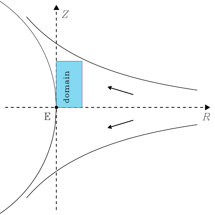
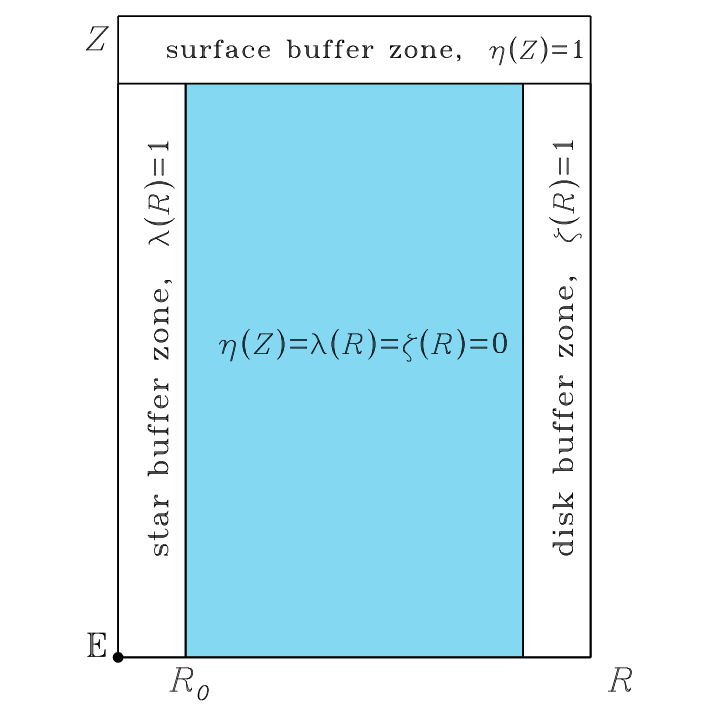
A sketch of the boundary layer on the surface of the neutron star is presented in Fig. 1. The gas is accreting in the disk mostly in the radial direction and turns in the -direction near the equatorial point . Since the purpose of this paper is to study the gas flow in the vicinity of , we use cylindrical coordinates, and neglect the curvature of the stellar surface. We consider a 2D domain limited in the radial direction by the surface of the star and the disk zone, where the rotational velocity is close to the Keplerian value (see Fig. 2).
| quantity | case 1 | case 2 | |
|---|---|---|---|
| cm | cm | ||
| M⊙ | 1.4 M⊙ | ||
| K | K | ||
| K | K | ||
| g cm-3 | g cm-3 | ||
| 107, 108 cm2 s | 1010 cm2 s-1 | ||
| 0 | 1 |
is a stellar radius, is stellar mass, and are temperatures of the star surface and the gas in the disk zone, is the gas density at the mid-plane in the disk zone, is a turbulent viscosity.
3 Boundary conditions and buffer zones
The boundary conditions represent an integral part of the overall solution in that the values on the boundaries both determine and depend themselves on the final solution. They must allow the accretion onto the stellar surface and the emission of energy. They must also simulate the compression of gas near the surface and allow this gas to become part of the surface, while the gas settling depends itself on the input parameters of incoming gas and conditions on the stellar surface. The rotational velocity of the gas in the disk part is close to Keplerian, but cannot be exactly Keplerian, because otherwise accretion would stop and the boundary layer would disappear. On the other hand, the deviation from the Keplerian velocity is determined by the conditions on the stellar surface. To cope with these complications we use so-called buffer zones, which are narrow regions just outside the domain (of the size of typically 5 grid-points; see Fig. 2), where additional terms are added to the hydrodynamical equations. This type of approach has proven to be useful in earlier simulations of disk outflows and star-disk coupling (von Rekowski et al., 2003). We use three different buffer zones that are characterized by the three profile functions for the disk buffer zone, for the star buffer zone, and for the surface buffer zone. In the following we describe the properties of these three zones separately.
In the disk buffer zone, where , the gas is accelerated close to the Keplerian speed due to an additional source term in the equation for , while adjusts itself to the conditions inside the domain. Thus, the and components of equation (2) are modified by additional terms on their right hand sides,
| (5) | |||
| (6) |
where denotes the meshpoint in the direction, is total number of the grid points in the -direction, and dots indicate the presence of terms that where already specified in equation (2). We take , where is the length of the time step.
In the buffer zone near the star, where , the radial gas velocity goes down to zero at the stellar surface. To describe the rotation of the star we introduce the parameter , which equals zero if the star is non-rotating one, and unity if it rotates with the corresponding Keplerian velocity. Thus the and components of equation (2) are modified further by the terms
| (7) | |||
| (8) |
where in the buffer zone, and zero outside.
The surface buffer zones will be discussed separately in the following two sections, because they have to be treated differently for gas and radiation pressure dominated regimes.
The temperatures on the stellar surface and the disk (left and right boundaries of the domain) are fixed by and , respectively, while the gas density is extrapolated on both sides. On the lower boundary of the domain (mid-plane of the disk) we use antisymmetric boundary conditions for the -component of the velocity and symmetric boundary conditions for all other quantities, while on the upper domain boundary all quantities are extrapolated. The turbulent viscosity is assumed to be constant everywhere in the domain.
For all simulations presented here we use the Pencil Code,11 1 http://www.nordita.dk/software/pencil-code which is a high-order finite-difference code (sixth order in space and third order in time) for solving the compressible hydrodynamic equations (Brandenburg & Dobler, 2002).
4 Gas pressure dominated case
As a first test we consider a gas pressure dominated case and choose the gas temperature in the disk to be K. This means that the radiation pressure is about two orders of magnitude smaller than the gas pressure. Also, we take the stellar mass to be so as to balance the gravity force near the surface by the gas pressure force. In addition, we assume that the star does not rotate (). We consider two cases with and cm2 s-1.
Since initially the disk is assumed to be in vertical hydrostatic equilibrium, the vertical velocity should be close to zero. In addition, we let the gas density approach a certain vertical profile , where the value at the disk mid-plane is g cm-3, and assume that decreases exponentially with . However, since the temperature profile results from a thermal balance between viscous heating and radiative cooling, the local sound speed in Eq. (9) is recalculated at each time step. This allows the vertical density profile to adjust to the conditions inside the domain. Thus, we have in the disk buffer zone
| (9) | |||
| (10) |
where
| (11) |
where in the disk buffer zone, and zero outside.
In the surface buffer zone, where , we assume vanishing first derivatives for all three velocity components () and for the specific entropy. We also correct the density profile to account for the resulting artificial pressure force which works against the vertical gravity. Due to this term, the gas flows out through the surface boundary rather than coming into the domain at the beginning of the calculation. Thus, we add the terms
| (12) | |||
| (13) | |||
| (14) |
We consider two runs with and cm2 s-1 and show in Fig. 3 two cross-sections respectively for m and 2 m, cm2 s-1 and cm2 s-1, and m in both cases. In Fig. 4 we show velocity and density. One can see that the accreting gas comes to the stellar surface and turns toward the poles of the neutron star.

.
We find that the size of the boundary layer, where the rotational velocity of the gas decreases from the Keplerian value down to zero, strongly depends on the value of the turbulent viscosity. The boundary layer becomes 3.5 times thicker if one increases by a factor of 10. This is consistent with the classical theory of a boundary layer, according to which the thickness of the boundary layer is inversely proportional to the square root of the Reynolds number, (Shih-I Pai, 1962, see, for example, ). The increase of viscosity also leads to a growth of the gas temperature, resulting from a balance between turbulent viscous friction and radiative cooling. One can see that the temperature achieves its maximal value in the middle of the boundary layer, where the velocity gradient and therefore the heating rate are maximum.
Note, that the solution for our test case looks similar to the spreading layer model for the white dwarf case. We find that the -component of the gas velocity cm s-1 is very close to that obtained by Piro & Bildsten (2004). Unfortunately, we cannot compare other quantities because the values in the spreading layer model are averaged along the -direction.
5 Radiation pressure dominated case


Let us now consider a realistic neutron star mass, . We find that, in order to balance the gravity force by the gas pressure gradient near the stellar surface, the gas temperature must attain a value of K, which is unrealistic. Therefore, in the case of a non-rotating star, the only force which can work against gravity is the radiation pressure gradient. Indeed, if one takes the gas temperature to be K and g cm-3, the radiation pressure force becomes comparable to the gravitational force (i.e. , where is the Stefan-Boltzmann constant).
Using standard disk theory, we estimate the turbulent viscosity near the stellar surface cm2 s-1, where is a viscosity parameter, , and cm s-1. Note, that the radiative viscosity cm2 s-1 (where is a proton mass) is much smaller than the turbulent one, and can be neglected.
We find that the description of buffer zones must be modified in the radiation pressure dominated case. For simplicity we use a similar density profile in the disk buffer zone as it was in the gas pressure dominated case. However, we now take g cm-3 and fix the gas temperature to avoid large radiation pressure gradients and therefore the generation of large velocities, which lead to strongly non-stationary behavior in the buffer zone and eventually to numerical instability. Also, we use a softer condition for the -velocity by assuming vanishing first derivatives. Thus, we set
| (15) | |||
| (16) | |||
| (17) |
In the course of the calculation we find that inside the domain cold low-density patches surrounded by denser hot gas appear sporadically. Such patches are dispersed due to motion of the gas from the core of the patch outward through the radiation pressure gradient. However, if we were to fix the and velocities in the star buffer zone to zero, such a patch cannot disappear, while the density inside this patch is going to decrease together with the temperature, and a numerical instability develops. To avoid this we use symmetry conditions relative to the inner boundary of the buffer zone (see Fig. 2) for , and . In addition we assume at . Thus, we have in the star buffer zone
| (18) | |||
| (19) | |||
| (20) |
Since the main goal of this paper is to consider the gas flow in the vicinity of the equatorial point , we consider a domain located inside the disk with a vertical size smaller than the height where the gas becomes cold and optically thin. To imitate a disk photosphere in the surface buffer zone we include an additional cooling term to create a vertical temperature gradient and to allow gas to escape through the surface boundary.
First, we attempt to consider a non-rotating star. It turns out that in this case the initial distribution of the main quantities (temperature, density, and velocity) have to be close to the final state, because otherwise inhomogeneities in the temperature result in large radiation pressure gradients which, in turn, generate large local velocities. Such velocity perturbations may produce a local decrease of density, which will lead to a decrease in radiative cooling, and hence to an increase in temperature. The resulting radiation pressure gradient will decrease the density even further, which leads therefore to an instability. (Note that this does not happen in the case of a smaller gas temperature because then the gas pressure dominates over the radiation pressure.)
Finding suitable initial conditions is a difficult task. It turns out that it is easier to consider first a rotating star, and then to decrease its rotational velocity down to the necessary value. However, the final rotational velocity still has to be considerable so that centrifugal and gravitational forces are of the same order of magnitude. In the opposite case, i.e. when the star is almost non-rotating, the gravity force has to be balanced by the radiation pressure gradient, which, in turn, should be negative near the stellar surface. However, it is not clear how to realize this, because the main heating mechanism is due to viscous friction which is maximum in the middle of the boundary layer rather than at the stellar surface.
At the current stage we assume that the rotational velocity of the star corresponds to the Keplerian velocity at the stellar radius (i.e. ). Also, we take a uniform initial distribution of temperature in the direction. In that case, at the beginning of the calculation, the huge gravitational force near the stellar surface is balanced by the centrifugal force. Depending on the temperature gradient, the -component of the radiation pressure force nearly vanishes and the resulting component of the velocity appears to be small.
While the component of the gravitational force is much smaller than the component, its influence on the gas motion in the direction is crucial and leads to strong flow of gas into the domain through the surface boundary and to an accumulation of gas near the equatorial point . To avoid numerical problems, we assume that initially the component of gravitational force is balanced by the corresponding component of the radiation pressure force. Therefore, the initial distribution of temperature takes the form
| (21) |
where is the size of the mesh in the direction. We use the same initial density distribution as in the gas pressure dominated case (see Sec. 4).
In Fig. 5 we present temperature and velocity fields (see also the sketch in Fig. 1). Here we show temperature rather than density (as was done in Fig. 4), because in the radiation pressure dominated case the flow of the gas is mostly determined by the radiation pressure force and hence by the temperature distribution. In addition, we take a larger domain size because the thickness of the boundary layer now appears to be an order of magnitude larger than that in Sec. 4.
The results of the calculation are also presented in Fig. 6, where density, temperature, and velocity of the gas are shown as functions of for three different distances from the mid-plane, , 50 and 110 m. We find that at higher latitudes the gas rotates with a velocity that is comparable to the rotational velocity of the star, while in the equatorial plane its rotational velocity is smaller than the stellar surface speed. This means that in the equatorial plane the centrifugal force is larger than the gravitational force, while at the higher latitudes the centrifugal force is smaller than the gravitational force. Such a relation between the main forces would result in accretion in the equatorial plane and excretion at higher latitudes, provided the gas pressure was much larger than the radiation pressure. However, since now the radiation pressure dominates, we obtain the opposite result: the gas accretes only at higher latitudes, while in the equatorial plane it is excreting.
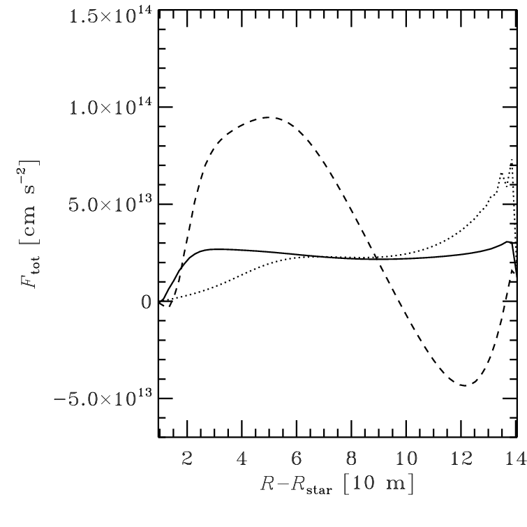
In Fig. 7 we present, as a function of , the sum of the components of gravitational, centrifugal, and radiation pressure forces, . One can see that at a higher latitudes the total force is at some radius negative, , so the generated radial velocity is negative (), which means accretion, while in the equatorial plane and , so the gas is excreting. The dominant role of the radiation pressure in driving the velocity field is also clear from analyzing the temperature in Fig. 5. One can see that the temperature decreases outward in the equatorial plane and increases outward at m near the disk buffer zone. Note that along the stellar surface the temperature is almost constant, so the component of the gravitational force dominates here, and causes the gas to sink toward the equatorial plane.
6 Conclusions
We have studied the gas flow in close vicinity of a neutron star in a low mass X-ray binary and have assumed that the magnetic field is negligible. The main purpose of this work was to investigate the flow near the equatorial plane between disk and star, so the curvature of the stellar surface in the latitudinal direction was neglected and cylindrical coordinates were used.
In the unrealistic, gas pressure dominated case the gas temperature is K (which is about an order of magnitude smaller than the observed value). If the star does not rotate, the gravitational force at a radius close to the stellar surface should be balanced by the gas pressure force. To have gas pressure and gravitational forces of the same order of magnitude, the stellar mass was chosen to be about two orders of magnitude smaller than the real mass of a neutron star. In this case the maximum release of energy occurs in the middle of the boundary layer, where the gas velocity gradient (and hence the viscous heating) reaches a maximum, while the radiation pressure force at the stellar surface is directed inward.
For a realistic neutron star mass, , the gas pressure gradient at the stellar surface becomes negligible compared with the gravitational force. The latter is balanced by the radiation pressure, so the gas temperature is about K. Unlike the gas pressure dominated case, the radiation pressure force is directed outward rather than inward. Thus, the maximum energy release occurs directly at the stellar surface. However, it is not clear how to realize such a scenario, where the gas is heated by viscous friction between the differentially rotating gas layers.
The picture becomes crucially different if one considers a rotating neutron star: the gravitational force can now be balanced by the centrifugal force. Here we have assumed that the neutron star rotates with the Keplerian velocity at the stellar radius. Alternatively, one might find a solution for smaller rotational velocities by gradually decreasing it down to the required value, using the result of calculating it for a larger velocity as an initial approximation for calculation with the smaller value.
We find that at higher latitudes the centrifugal force is larger than the gravitational force, while at the equatorial plane the gas rotates with a velocity that is considerably smaller than the corresponding Keplerian value. It would be reasonable to assume that the gas is accreting near the equator and excreting at higher latitudes. However, we find the opposite: the accretion occurs only at higher latitudes, while in the equatorial plane the gas is excreting. This is related to the temperature distribution, and therefore, to the radiation pressure force, which is now dominant. We find that near the equatorial plane the temperature decreases outward, so the gas is pushed away from the surface by radiation pressure. At higher latitudes, some distance away from the surface, the temperature decreases inward, resulting in accretion. The circulation of the gas is closed by a flow along the stellar surface from high to low latitudes, because the temperature is almost constant in this direction and the gas flow is controlled only by the tangential component of gravity.
Finally, one should note that, since we have considered only a laminar two-dimensional model of the boundary layer at the neutron star surface, we have assumed that the turbulent viscosity is constant everywhere and that it can be treated as an input parameter. Future three-dimensional simulations will allow us to model turbulent processes more accurately. However, even the results of the two-dimensional simulations give us some clues for understanding the physical processes near the neutron star surface. These results can in principle be used for a more detailed description of the vertical structure of the boundary layer and for calculating spectra of neutron star radiation. Furthermore, the presented results may be useful for understanding the nature of quasi-periodic oscillations.
Acknowledgments
This work was supported by the Academy of Finland grant 110792 and the Magnus Ehrnrooth Foundation. We acknowledge the allocation of computing resources provided by the Center for Scientific Computing in Finland.
References
- Barret et al. (2000) Barret D., Olive J. F., Boirin L., Done C., Skinner G. K., Grindlay J. E., 2000, ApJ, 533, 329
- Brandenburg & Dobler (2002) Brandenburg A., Dobler W., 2002, Comp. Phys. Comm., 147, 471
- Inogamov & Sunyaev (1999) Inogamov N. A., Sunyaev R. A., 1999, Astron. Lett., 25, 269
- Medvedev (2004) Medvedev, 2004, ApJ, 613, 506
- Gilfanov et al. (2003) Gilfanov M., Revnivtsev M., Molkov S., 2003, A&A, 410, 217
- Mitsuda et al. (1984) Mitsuda K. et al., 1984, PASP, 36, 741
- Narayan & Popham (1993) Narayan R., Popham R., 1993, Nature, 362, 820
- Piro & Bildsten (2004) Piro A. L., Bildsten L., 2004, ApJ, 610, 977
- Popham & Narayan (1992) Popham R., Narayan R., 1992, ApJ, 394, 255
- Pringle (1977) Pringle J. E., 1977, MNRAS, 178, 195
- van der Klis (2000) van der Klis M., 2000, ARA&A, 38, 717
- Shih-I Pai (1962) Shih-I Pai, 1962, Introduction to the theory of compressible flow. Van Nostrand, Princeton
- Sibgatullin & Sunyaev (1998) Sibgatullin N. R., Sunyaev R. A., 1998, Astron. Lett., 24, 774
- Suleimanov & Poutanen (2006) Suleimanov V., Poutanen J., 2006, MNRAS, 369, 2036
- Sunyaev & Shakura (1986) Sunyaev R. A., Shakura N. I., 1986, Sov. Astron. Lett., 12, 117
- von Rekowski et al. (2003) von Rekowski B., Brandenburg A., Dobler W., Shukurov A., 2003, A&A, 398, 825