$p$-wave phase shift and scattering length of ⁶Li

In this region, we can neglect the $k^{2}$ term

and hence, the solution is independent of $k$. At large distances from the scattering center, van der Waal’s potential $U(R)=-2m\alpha/(R^{6})=-\gamma^{2}/R^{6}$ is the dominant inter-atomic interaction. Here, $\alpha$ is the van der Waal’s coefficient. For low energy collisions $k\rightarrow 0$, the interatomic potential approaches the asymptotic form within the $kR\ll 1$ region. Then,

Substituting $\chi(R)=\xi(R)\sqrt{R}$ and $R=\sqrt{\gamma/2x}$, we obtain the Bessel differential equation of order $(2l+1)/4$

The general solution of Eq.(3) is

Considering the $p(l=1)$ partial wave

In the limit $R\rightarrow\infty$ or $x\rightarrow 0$, where $kR<1$, the leading terms in the series expansion of $J_{3/4}(x)$ and $J_{-3/4}(x)$ are dominant and the remaining terms are negligible

where $\Gamma(\ldots)$ are the gamma functions.

In this region, we can neglect the interatomic interaction potential $U(R)$, if it approaches zero faster than $1/R^{2}$. In addition, as in the $kR\ll 1$ region, the $k^{2}$ term can be neglected

The most general solution of this equation is

For $l=1$, comparing the solutions in Eq. (5) and Eq. (7)

The comparison is possible as $\chi$ in the $R\rightarrow\infty$ of Eq.(4) has the same form as the solution in the $kR<1$ region.

Increasing $R$ further, we enter the $kR\approx 1$ region. In this region, we can neglect $U(R)$ in comparison to the other terms in Eq. (1), then

This is the Schrödinger equation in the asymptotic region and the solution is a plane wave of wave number $k$. However, the interatomic potential introduces a phase shift ($\eta_{l}$)[15] to the plane wave

Expanding the Bessel’s functions $J_{l+1/2}(kR)$ and $J_{-l-1/2}(kR)$, the solution when $kR<1$ is

Equating the solutions in Eq. (7) and  (10)

Since $b/a$ is independent of $k$, $\tan\eta_{l}$ varies as $k^{2l+1}$. It should also be mentioned that, though the entire radial range is divided into three domains, the solutions are in the asymptotic region. This defines the phase shift $\eta_{l}$ in terms of the $b/a$ and it is strictly applicable for $k\rightarrow 0$. For the $p$-partial wave

In the above expression, to calculate $\eta_{1}$, the ratio $b/a$ should be determined. From the Eq.(8), the phase shift can also be defined in terms of $A/B$ as

Here the actual values of $\Gamma(3)$ and $\Gamma(4)$ are used. Now onwards this definition of $\eta_{1}$ is used. As the phase shift $\eta_{1}$ has functional dependence on $\tan^{-1}$, which has a domain of $[-\infty,\infty]$, its accuracy is sensitive to the value of $A/B$.

For partial waves other than $s$, the centrifugal potential is nonzero. Combining the the interatomic potential and centrifugal term, the effective interatomic potential

Then the local momentum of the scattered atom $p(R)=\sqrt{-U_{\rm eff}(R)}$, and the de Broglie wavelength $\lambda(R)=2\pi/\sqrt{-U_{\rm eff}(R)}$. The WKB approximation is applicable when

In above relation $F=-dU_{\rm eff}/(2mdR)$ is the net force acting on the atom. At large distances, when the interatomic potential approaches the asymptotic form, the above inequality for $l=1$ is

This inequality is in general valid up to large radial distances. As an example Fig.1 shows that for Cs the inequality is satisfied up to $\approx 30$. Then the WKB solution at $R$ which satisfies the inequality and larger then the classical turning point $R_{o}$ is

and the logarithmic derivative is

An analytic expression of $\zeta(R)$ for $l=1$ is obtained if only the van der Waal’s potential is considered

This approximation neglects the well and inner wall part of the interatomic potential. It is appropriate for model potentials comprising of the van der Waal’s and hard core potential. The above expression is reduced to that of $s$ case when $l=0$, which is used implicitly in ref. [12].

From the inequality (16), it is evident that when $\gamma$ is sufficiently large, WKB solution is valid up to radial distances where the asymptotic form of the potential begins to dominate. Choose a point $R^{*}$ in this region, such that the $2$ in the inequality can be neglected. Then the inequality is modified to

At this point, as the interatomic potential has the asymptotic form, Eq. (4) is a solution of the Schrödinger equation Eq.(1). This is discussed in Section.II.1.

From the definition, at $R^{*}$ and around it $x=\gamma/(2R^{*2})\gg 1$. Where $x$ is the variable first used in Section II.1. We can then use the asymptotic expression expression of the Bessel’s function

and the solution in Eq. (4) is

This is the inner limit of the asymptotic solution. Whereas the solution in Eq.(5), in the $x\rightarrow 0$, is the outer limit of the asymptotic solution. To determine $A/B$ we match the logarithmic derivatives of the analytical solution in Eq. (21) and WKB solution in Eq. (17). The ratio is

here $\phi_{1}=\gamma/(2R^{*2}-5\pi/8)$, $\phi_{2}=\gamma/2R^{*2}+\pi/8$. It is evident from the above expression that $A/B$ depends on the choice of the matching point $R^{*}$. This implies that $\eta_{1}$ and hence the scattering length, to be defined later, depend on $R^{*}$. This radial dependence arises from the centrifugal part in the expression of the effective potential $U_{\rm eff}(R)$. Neglecting the terms arising from the centrifugal potential in the expression of $\zeta(R)$, logarithmic derivative of the WKB solution is

For the obvious reason, large value of $R/\gamma$, this expression is not valid at very large values of $R$. Assuming that the maximum radial distance at which the above expression is valid, the interatomic potential has the asymptotic form. If $A/B$ is calculated using Eq. (23) as the WKB solution, it is then independent of the choice of matching point

where $\phi=\gamma/(2R_{o}^{2})$. This is however a crude estimate as the outer solution includes the effect of centrifugal term but the inner solution, the WKB solution, does not. Still, it is a useful estimate, as it is an analytic expression and not difficult to evaluate.

For any arbitrary potential which vary as $R^{-n}$, the scattering length ($a_{l}$) and phase shift ($\eta_{l}$) are related as [15]

This relation is valid provided $l<(n-3)/2$ and is applicable for $p$ partial wave when $n=6$ or higher. From Eq. (13) and (25) scattering length of the $p$ partial wave is

Using the value of $A/B$ in Eq.(22), the $p$-wave scattering length $a_{1}$ can be evaluated. A rough estimate of $a_{1}$ is to use the analytical expression in Eq.(24). The quantity $a_{1}^{3}$ is referred to as the $p$wave scattering volume. It is an important parameter in the three-body recombination of identical, spin polarized fermions in low tempertures [16].

Consider the scattering of two Cesium atoms in the ${}^{3}\Sigma_{u}$ state . The form of interaction potential is [17]

where $B=0.0016$, $\alpha=5.53$ and $\beta=1.072$. These are given in ref [12] and $f_{c}(R)$ is the cut-off function and has the expression

where $\Theta(\ldots)$ is the step function which is equal to $1$ or $0$, depending on whether its argument is greater or less than zero. Here $R_{c}$ is the cut off parameter.

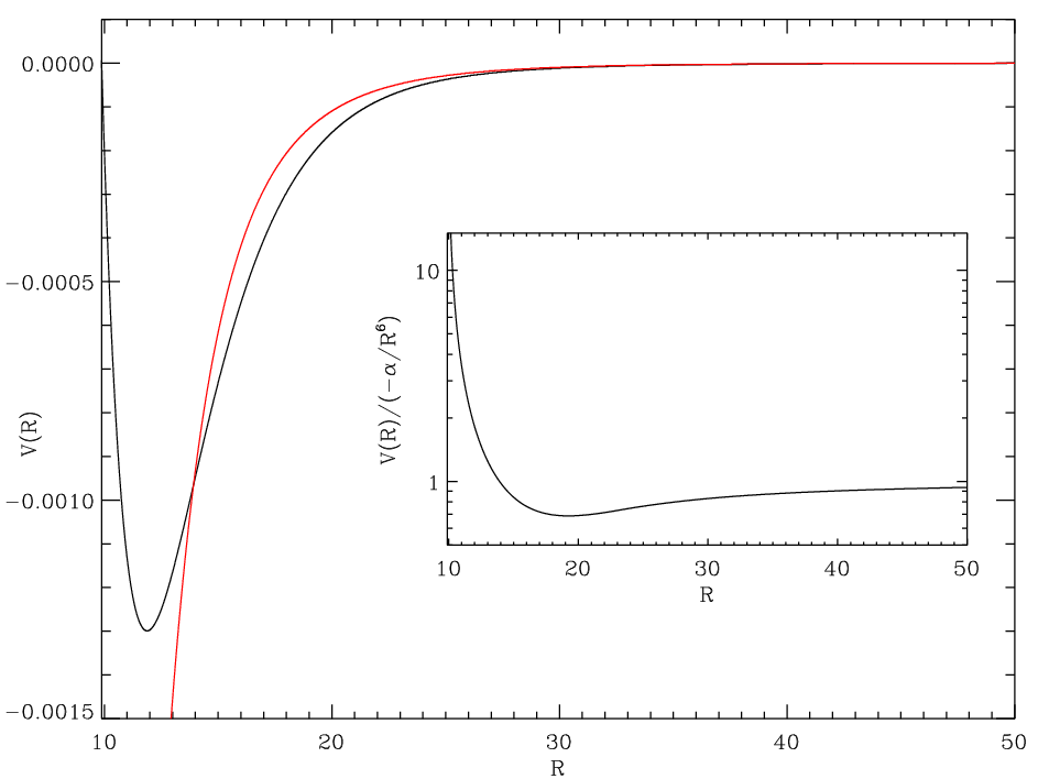
For comparison, the total interatomic potential $V(R)$ and van der Waal’s potential are shown in Fig.3. The ratio of the two are also shown as an inset plot. The figure shows that $V(R)$ approaches the asymptotic form at around $R=24$, where the ratio of the two is $0.8$. Beyond $R=30$, the two are indistinguishable. Using this potential, the phase shift and scattering lengths are calculated for the ¹³²Cs and ¹³⁴Cs fermionic isotopes. As test calculations, we evaluated the $s$ wave phase shifts for the ¹³³Cs isotope. It is to be mentioned that, the value of $\gamma$ is 41240.1. However, in ref. [12] the value of $\gamma$ is defined as 41200. Using the later, the results of the test calculations are in good agreement with that of ref. [12].

From Eq .(24), which provides a rough estimate, the value of $a_{1}$ is $137$a.u and $-108$ a.u. for ¹³²Cs and ¹³²Cs respectively.

The $\eta_{1}$ calculated from the variable phase method, for different $R_{c}$ for a range of $k$ close to zero are shown in Fig.4. Our calculations show that, the value of $\eta_{1}$ at higher values of $k$ are sensitive to $\gamma$, the dependence is nonlinear as the equation of phase function is a nonlinear differential equation. Consequently, small change in $\gamma$ could result in significant change of $\eta_{1}$. The dependence $\eta_{1}$ on $\gamma$ for larger difference is evident from Fig.4, which shows $\eta_{1}$ for ¹³²Cs and ¹³⁴Cs. The difference in the interatomic potential of the two isotopes is the mass, which manifests as unequal values of $\gamma$. There are two distinct differences in the results for the two isotopes: for the $R_{c}=23.215$ case $\eta_{1}$ converges to $179.08$ and $182.21$ for ¹³²Cs and ¹³⁴Cs respectively; and for the $R_{c}=23.115$ case $\eta_{1}$ converges to $182.22$ and $185.35$ respectively. The phase function in the neighborhood of $k=0$ is also sensitive to the accuracy of the integration.

In the present calculations, the phase function equation is integrated till $\eta_{1}$ converges to the order of $10^{-6}$, which is consistent with the choice of tolerance. For Cs, this requires integration up to radial distances of $\sim 500$. The large radial distance is necessary as the phase shift is an asymptotic property. In addition, for the $p$ wave scattering the centrifugal potential, which has $R^{-2}$ dependence, vanishes at a slower rate compared to the van der Waal’s potential at large radial distances. This slows the convergences of the phase shift. A calculation of the $s$ wave phase shift confirms this. The $s$ wave phase shift $\eta_{0}$ converges to the order of $10^{-6}$ when the phase equation is integrated to a radial distance of $\approx 100$.

The values of $-\tan(\eta_{1}(k))/k^{3}$ for ¹³⁴Cs within a range of $k$ for different $R_{c}$ are shown in Fig.5. As discussed in ref. [12], the $R_{c}=23.165$ is a physically reasonable choice. For this the scattering length calculated as the slope of $-\tan(\eta_{1})/k^{2}$ in the $k\rightarrow 0$ are $53$ and $-113$ in atomic units for ¹³²Cs and ¹³⁴Cs respectively. This differs from the analytic values mentioned earlier by 61% and 4.4% for ¹³²Cs and ¹³⁴Cs respectively. It shows that the analytic expression though crude provides a good estimate for ¹³⁴Cs, which has higher $\gamma$ .

The evaluation of $\eta_{1}$ from the numerically calculated $A/B$ poses some difficulty. This is to do with the choice of appropriate $R^{*}$, the matching point, the dependence is shown in the Fig.6. The over all trend of the variation is rather complicated for the actual interatomic potential but less when only the van der Waal’s potential is considered. However, it is possible to calculate $A/B$ from the value of $a_{1}$ calculated earlier, which is obtained from the variable phase method. The value of $A/B$ obtained from such a calculation are $\approx-0.109$ and $\approx 1.042$ for ¹³²Cs and ¹³⁴Cs respectively.

The value of $R^{*}$ around which $A/B$ is close to this value occurs around the radial range of $23-24$ atomic units. This is not surprising, as mentioned earlier, this is the radial range where the interatomic potential approaches the asymptotic form.

For the $a^{3}\Sigma^{+}_{u}$ state of ${}^{6}\rm{Li}_{2}$, we use the interatomic potential suggested by Zemke and Stwalley [18]. The long range part of the interaction potential, for ⁷Li in particular, are discussed in ref. [14]. For the $R\leq 6.388674$ and $R\geq 18.0$ regions, the analytic expressions recommended in ref. [18] are used. Then, for the $6.388674<R<18.0$ region, the interatomic potential is approximated as the cubic spline fitted to the potential values given by Zemke and Stwalley. A plot of the interatomic potential obtained is shown in Fig.7.

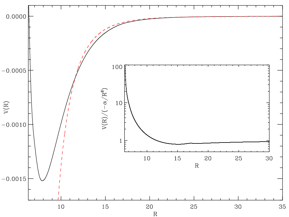
As to be expected, the potential approaches the asymptotic form, van der Waal’s potential, at smaller radial distance compared to Cs. This is evident from a visual comparison of the two potentials shown in Fig.7 and Fig.3. This implies that, the phase shift calculation of lithium can have better convergence properties. Consequently, the methods adopted for the Cs calculations are applicable to Li and provide results with higher accuracy.

To optimize the calculations, we use the RKF method to solve Eq.(28) with relative tolerance varied as a function of $k$. The relative tolerance is set to $10^{-5}$ for $k>0.01$ and it is lowered as $k$ is decreased. This is essential as the scattering length depends on the nature of the phase shift in the neighborhood of $k=0$. Based on extensive test calculations, the optimal choice of the relative tolerance is $10^{-6}$ for $0.01\leq k<0.005$ and $10^{-7}$ for $k\leq 0.005$. With this choice it is possible to get reliable results for phase shift up to $k=0.0005$. We find that phase shift stabilizes to $31.46$ as $k\rightarrow 0$ which is shown in Fig.8.

The sensitivity of the phase shift to the relative tolerance at low $k$ is not very prominent from the values of $\eta_{1}$. However, it is not so with the $-\tan(\eta_{1})/k^{3}$, which is the scattering length in the $k\rightarrow 0$ limit. The small value of $k$ and the transcendental function $\tan$ enhances variations in $\eta_{1}$. This is evident when $-\tan(\eta_{1})/k^{3}$ as a function of $k$ is compared at low $k$ values for two different relative tolerances. The plot of such a comparison is shown as the inset plot in Fig.9. With improved tolerance, the lowest $k$ value up to which the reliable phase shift can be calculated is decreased. There is however a limitation to decreasing the value of $k$, up to which the phase shift is calculated, by decreasing the value of relative tolerance. Below a certain value of relative tolerance, the RKF method fails to perform the integration of the phase equation up to the cut off point.

From the calculations, we find that $-\tan(\eta_{1})/k^{3}$ stabilizes to $\approx-92660$ , this is evident from the plot in Fig.9). The cube root of this is the $a_{1}$. Another equivalent way to calculate the scattering length is to evaluate the slope of $-\tan(\eta_{1})/k^{2}$ in the $k\rightarrow 0$ limit. We calculate this by least square fitting the data points for $-\tan(\eta_{1})/k^{2}$ between $0.005\leq k\leq 0.0005$ with an additional point corresponding to zero phase shift at $k=0$.

As is evident from Fig.(10) there is very good fitting of straight line over the data points. The slope of the least square fitted line is $-92600$, the cube root of which is $-45$ and can be considered as a reliable value of the $p$-wave scattering length. If we compare it with the analytic approximation of $a_{1}$ obtained by using Eq .(24) as the value of $A/B$, we find that percentage error incurred by using analytic approximation is $43.74$ percent.

References

- [1] B. DeMarco and D. S. Jin, Science 285, 1703 (1999).
- [2] H. T. Stoof, M. Houbiers, C. A. Sackett, and R. G. Hulet, Phys. Rev. Lett. 76, 10 (1996); M. Houbiers, R. Ferwerda, H. T. C. Stoof, W. I. McAlexander, C. A. Sackett, and R. G. Hulet, Phys. Rev. A 56, 4864 (1997).
- [3] J. Kinast, S. L. Hemmer, M. E. Gehm, A. Turlapov, and J. E. Thomas, Phys. Rev. Lett. 92, 150402 (2004).
- [4] M. Bartenstein, A. Altmeyer, S. Riedl, S. Jochim1, C. Chin, J. H. Denschlag, and R. Grimm, Phys. Rev. Lett. 92, 203201 (2004).
- [5] M. W. Zwierlein, J. R. Abo-Shaeer, A. Schirotzek, C. H. Schunck and W. Ketterle, Nature 435, 1047 (2005).
- [6] M. M. Parish, F. M. Marchetti, A. Lamacraft and B. D. Simons, Nature Phys. 3, 124 (2007).
- [7] Y. Shin, C. H. Schunck, A. Schirotzek and W. Ketterle, Nature bf 451, 689 (2008).
- [8] M. Taglieber, A.-C. Voigt, T. Aoki, T. W. Hänsch, and K. Dieckmann, Phys. Rev. Lett. 100, 010401 (2008).
- [9] M. M. Parish, F. M. Marchetti, A. Lamacraft, and B. D. Simons, Phys. Rev. Lett. 98, 160402 (2007).
- [10] Z. Idziaszek and T. Calarco, Phys. Rev. Lett. 96, 013201 (2006).
- [11] K. Kanjilal and D. Blume, Phys. Rev. A 70, 042709 (2004).
- [12] G. F. Gribakin and V. V. Flambaum, Phys. Rev. A 48, 546, (1993).
- [13] F. Calogero, Variable phase approach to potential scattering (Academic Press, New York, 1967).
- [14] R. Côté, A. Dalgarno and M. J. Jamieson, Phys. Rev. A 50, 399 (1994).
- [15] N. F. Mott and H. S. W. Massey, The theory of atomic collisions (Oxford University Press, 1965).
- [16] H. Suno, B. D. Esry and C. H. Greene, Phys. Rev. Lett. 90, 053202 (2003).
- [17] A. A. Radstig and B. M. Smirnov, Parameters of Atoms and Atomic Ions Handbook, (Energoatomizdat, Moscow, 1986).
- [18] W. T. Zemke and W. C. Stwalley, J. Phys. Chem. 97,2053-2058, (1993)
- [19] W. T. Zemke and W. C. Stwalley, J. Chem. Phys. 100, 2661 (1994).
- [20] W. T. Zemke, C-C. Tsai and W. C. Stwalley, J. Chem. Phys. 101, 10382 (1994).