Massive Charged Scalar Quasinormal Modes of Reissner-Nördstrom Black Hole Surrounded by Quintessence
Abstract
We evaluate the complex frequencies of the normal modes for the massive charged scalar field perturbations around a Reissner-Nördstrom black hole surrounded by a static and spherically symmetric quintessence using third order WKB approximation approach. Due to the presence of quintessence, quasinormal frequencies damp more slowly. We studied the variation of quasinormal frequencies with charge of the black bole, mass and charge of perturbating scalar field and the quintessential state parameter.
1 Introduction
It is now well understood that different kinds of perturbations in the geometry of a black hole can excite certain combination of its characteristic complex frequencies of the normal mode, called quasinormal modes(QNMs), whose real part represents the ring down frequency and imaginary part, the decay time and they are independent of the initial perturbation, but depends only on the parameters of black hole. The concept of QNM is put forward by Vishweshwara[2] and since then the quasinormal spectrum of black holes has been extensively studied for a great verity of black hole back grounds and perturbation fields because of its astrophysical and other theoretical interests. Astrophysical interests are associated with their relevance in gravitational wave analysis[3]. The QNMs of black hole are expected to be detected by the future gravitational wave detectors such as LISA[15], and give an opportunity to explore the properties of black holes directly. Apart from the observational interest of detection of quasinormal ringing by gravitational wave detectors, study of QNM found significance in AdS/CFT correspondence[17], black hole area quantization and Loop Quantum Gravity[16].
The idea that our universe is in a phase of accelerated expansion rather than holding steady, is strongly supported by a set of recent interlocking observations such as studies of distant supernovae[1], type 1a supernova[4] and cosmic microwave background radiation anisotropy[5], indicating the presence of some mysterious form of repulsive gravity called dark energy. In order to explain the nature of dark energy several models were proposed(for a recent review see[6]). The simplest option for this dark energy is Einstein’s cosmological constant[7] with a constant equation of states(EOSs) but it needs extreme fine tuning to account for the observations. The second is the dynamical scalar field models like quintessence[8], k-essence[9] and phantom[10], in which the EOSs of dark energy changes with time. Among them, the quintessence is the most natural model, and can give the EOSs with .
Because of relevance of the two topics, some studies of QNMs of black hole were started in the presence of quintessence, after Kiselev[18] derived the exact solution of Einstein equation for quintessential matter surrounding a black hole. QNMs of Schwarzschild black hole is studied for scalar[11], gravitational[12], electromagnetic[13] and massless Dirac field[14] perturbations in the presence of quintessence. Our work extend the studies to charged black hole space times. Charged scalar QNMs of Reissner-Nordstrom black hole were studied in[23, 24]. In this paper we considered the perturbation of Reissner-Nordstrom black hole encircled by quintessence for massive charged scalar field perturbations and study the dependence of quasinormal spectrum upon different parameters of the problem such as charge of the black bole, mass and charge of perturbating scalar field and the quintessential state parameter.
2 Massive charged scalar field around a Reissner-Nordstrom black hole surrounded by quintessence
Kiselev derived a static spherically symmetric exact solution of Einstein equations for quintessential matter surrounding a charged black hole under the condition of additivity and linearity in energy momentum tensor[18]. The metric can be expressed in the form
| (1) |
where
with and mass and charge of the black hole. is the quintessential state parameter and is the normalization factor which depends on ,the density of quintessence. The Klein-Gordon equation describing the evolution of massive charged scalar perturbation field outside a charged black hole is given by[19]
| (2) |
where is the electromagnetic potential and is the charge of the scalar field. Representing the charged scalar field in to spherical harmonics
| (3) |
the wave equation becomes
| (4) |
where we used the coordinate transformation defined by
| (5) |
The electromagnetic potential ,where is a constant. We define
| (6) |
to avoid the physically unimportant quantity . where is the radial part of perturbation variable taken to have time dependence . Now the radial perturbation equation can be written as
| (7) |
where and is the scattering potential, which is a function of frequency of perturbation, and is given by
| (8) |
3 Evaluation of Quasinormal modes
We use the third order WKB approximation method to determine the complex normal mode frequencies of black hole, a semi analytic method originally developed by Schutz and Will[20] for the lowest order. Later Iyer and Will[21] carried this approach to third WKB order and Konoplya[22] to sixth order to get more accurate results.
It gives a simple condition which will lead to discreet, complex values for the normal mode frequencies.
| (9) |
where and are higher order terms given by
| (10) |
| (11) | |||||
where
denotes the nth derivatives of evaluated at , the value of at which attains maximum. Here a complexity arises from the fact that the potential is a function of frequency . This makes difficult to calculate the value of . We make use of the procedure suggested by Konoplya[23] to find by fixing all the parameters other than for which the depends and then find the value of at which attains maximum as a numerical function of . Substitute for and then find the value of which satisfies the condition (9) by trial and error way.
4 Results and Discussion
We take all the values of parameters in black hole mass(M) units. It is a general experience that the imaginary part of quasinormal frequencies decreases with increase in mode number, , means that the quasinormal frequencies with lower mode number will decay slowly and are relevant to the description fields around black hole. So we consider frequencies for lower mode number for our study. The dependence of real and imaginary parts of on the charge of the black hole, is plotted in Figure1 for fixed and for different values of with . The case with absence of quintessence is also plotted (dotted line).
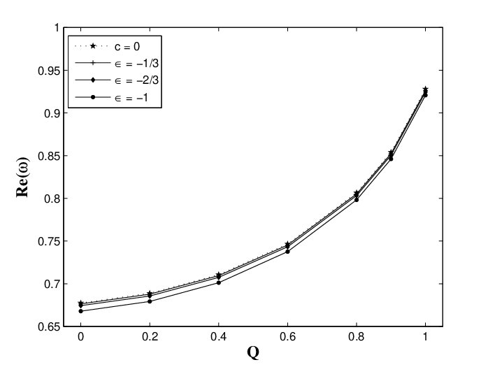
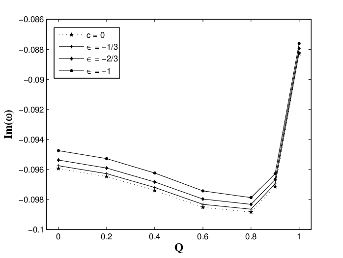
The quasinormal frequencies for scalar field in charged black hole is influenced by quintessence. The magnitudes of real and imaginary parts of is lower in the presence of quintessential field. This implies due to the presence of quintessence, the quasinormal frequencies for scalar field in RN black hole damps more slowly. As in the absence of quintessence[23, 24], increases monotonically with the increase in while the magnitude of first decreases, falling to a minimum around and thereafter increases sharply. For larger values of , the modification with quintessence decreases.
Figure2 shows the variation of and with quintessential state parameter with for fixed . As the value of increases increases slowly but the magnitude of increases more fast, means damping is less for lower values of .
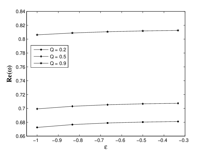
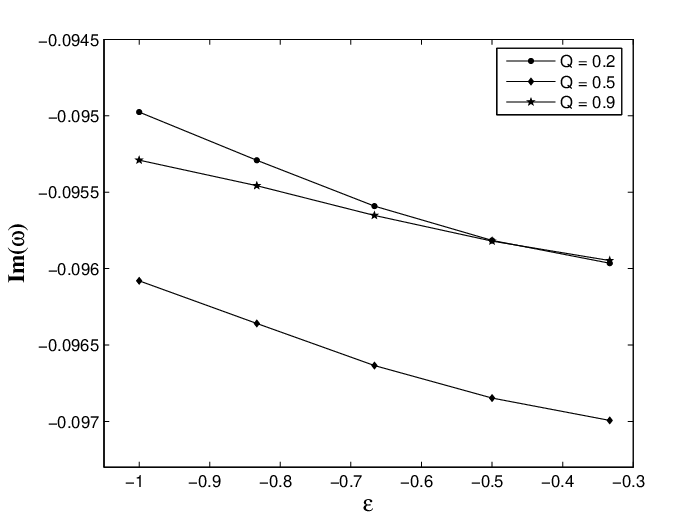
In Figure3 and are plotted as functions of with for and different values of . Dotted line represents absence of quintessence(c=0). The variation is almost linear. In the presence of quintessence, the magnitude of and increases with imitating the no quintessence case but with lower values of and . The modification with becomes larger for higher values of .
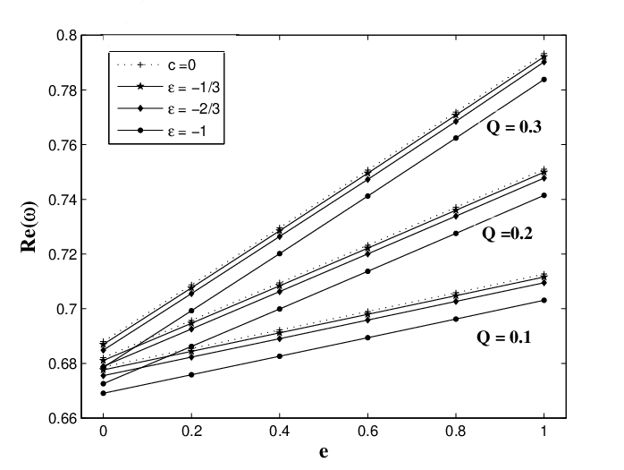
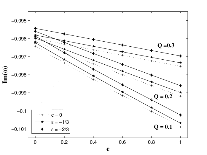
Finally, we study the role of mass of scalar field on quasinormal frequencies. Quasinormal modes occur only when the peak value of the potential is larger than and of the field is smaller than this peak value[25]. This means that there exists a maximum value for mass, beyond which there will be no quasinormal modes. can be estimated from the condition for the existence of quasinormal modes,
| (12) |
The values of obtained for different values of is tabulated in Table1. In the presence of quintessence decreases because quintessence lowers the height of the potential barrier as shown in Figure5 and when , it has the lowest value.
| 0 | – | 0.88516 | 0.001 | -2/3 | 0.87815 |
|---|---|---|---|---|---|
| 0.001 | -1/3 | 0.88366 | 0.001 | -1 | 0.85864 |
The values of and evaluated using WKB method with the variation of mass is plotted in Figure4.
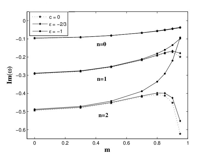
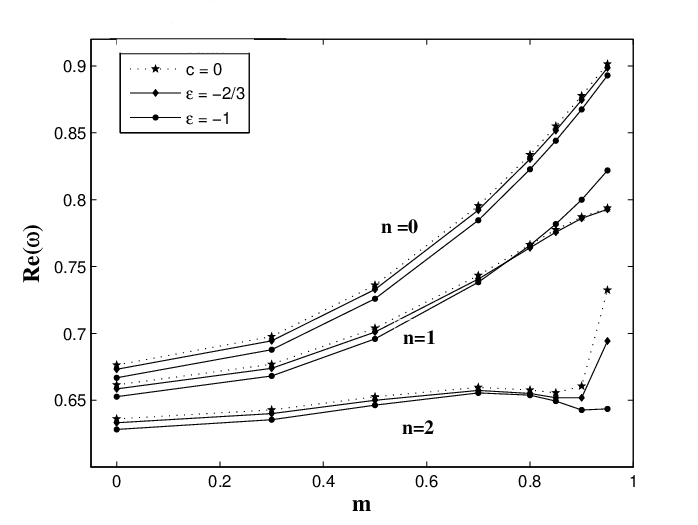

increases with increase in mass while decreases with mass, which indicates that QNMs of fields with lower mass damp slowly. But they behave abnormally near . This is due to the fact that, for larger mass of the field the potential looses its barrier shape by broadening the potential peak as shown in Figure5 and WKB method gives inaccurate results. Lower modes show less abnormality showing that WKB method is more accurate for fundamental modes.
Another thing we noticed is that this abnormal behavior is lower in the presence of quintessence and even when we can get satisfactory curve because the peak of effective potential broaden much less in the presence of quintessence comparing with the normal case(c=0) as understood from Figure5 and quintessence helps to retain barrier shape and give more accurate results at larger mass range.
5 Acknowledgment
VCK is thankful to U.G.C, New Delhi for financial support through a Major Research Project and wishes to acknowledge Associateship of IUCAA, Pune, India.
References
References
- [1] Guzzo L et al 2008 Nature 451 541.
- [2] Vishveshwara C V 1970 Nature 229 936.
- [3] Kokkotas K D and Schmidt B G 1999 Living Rev. Relativity 2 2.
- [4] Perlmutter S et al 1999 Astropphys. J. 517 565. Zhang X and Wu F Q 2005 Phys. Rev. D 72 043524.
- [5] Lamon R and Durrer R 2006 Phys. Rev. D 73 023507. Halverson N W et al 2002 Astropphys. J. 568 38. De Bernardis Pet al 2000 Nature 404 955.
- [6] E J Copeland, M Sami and Tsujikawa S 2006 Int. J. Mod. Phys. D 15 1753.
- [7] Padmanabhan T 2003 Phys. Rep. 380 235.
- [8] Ratra B and Peebles P J E 1988 Phys. Rev. D 37 3406. Sahni V and Wang L M 2000 Phys. Rev. D 62 103517. Caldwell R R, Dave R and Steinhardt P J 1998 Phys. Rev. Lett. 80 1582.
- [9] Chiba T, Okabe T and Yamaguchi M 2000 Phys. Rev. D 62 023511. Scherrer R J 2004 Phys. Rev. Lett. 93 011301.
- [10] Caldwell R R 2002 Phys. Lett. B 545 23. Vikman A 2005 Phys. Rev. D 71 023515.
- [11] Chen S and Jing J 2005 Class. Quantum Grav.22 4651. Ma C, Guy Y, Wnag W and Wang F 2006 arXiv:gr-qc 0611146v2.
- [12] Zhang Y and Gui Y X 2006 Class. Quantum Grav.23 6141.
- [13] Zhang et al 2007 Gen. Rel. Grav. 39 1003.
- [14] Zhang Y, Gui Y X and Yu F 2007 arXiv: 0710.5064v1. arXiv:0710.5064v1.
- [15] Berti E, Cordoso V and Will C M 2006 Phys. Rev. D 73 064030
- [16] Dreyer O 2003 Phys. Lett. 90 081301. Hod S 1998 Phys. Rev. Lett. 81 4293.
- [17] Cordoso V and Lemos J P S 2001 Phys. Rev. D 63 124015. Birmingham D, Sachs I and Solodukhin S N 2002 Phys. Rev. Lett. 88 151301. Whang B et al 2004 Phys. Rev. D 70 064025.
- [18] Kiselev V V 2003 Class. Quantum Grav.20 1187.
- [19] Hod S and Piran T 1998 Phys. Rev. D 58 024017.
- [20] Schutz B F and Will C M 1985 Astropphys. J. 291 L33-6.
- [21] Iyer S and Will C M 1987 Phys. Rev. D 35 3621.
- [22] Konoplya R A 2002 Phys. Rev. D 68 024018.
- [23] Konoplya R A 2002 Phys. Rev. D 66 084007.
- [24] Chang J F and Shen Y G 2007 Int. J. Theor. Phys. 46 1570.
- [25] Cho H T 2003 Phys. Rev. D 68 024003.