Learning Balanced Mixtures of Discrete Distributions
with Small Sample

\nameShuheng Zhou \emailszhou@cs.cmu.edu Affiliation: \addrComputer Science Department Affiliation: Carnegie Mellon University Affiliation: Pittsburgh, PA 15213, USA

Abstract

We study the problem of partitioning a small sample of $n$ individuals from a mixture of $k$ product distributions over a Boolean cube $\{0,1\}^{K}$ according to their distributions. Each distribution is described by a vector of allele frequencies in $\mathbb{R}^{K}$ . Given two distributions, we use $\gamma$ to denote the average $\ell_{2}^{2}$ distance in frequencies across $K$ dimensions, which measures the statistical divergence between them. We study the case assuming that bits are independently distributed across $K$ dimensions. This work demonstrates that, for a balanced input instance for $k=2$ , a certain graph-based optimization function returns the correct partition with high probability, where a weighted graph $G$ is formed over $n$ individuals, whose pairwise hamming distances between their corresponding bit vectors define the edge weights, so long as $K=\Omega\left(\ln n/\gamma\right)$ and $Kn=\tilde{\Omega}\left(\ln n/\gamma^{2}\right)$ . The function computes a maximum-weight balanced cut of $G$ , where the weight of a cut is the sum of the weights across all edges in the cut. This result demonstrates a nice property in the high-dimensional feature space: one can trade off the number of features that are required with the size of the sample to accomplish certain tasks like clustering.

Keywords: Mixture of Discrete Distributions, Graph-based Clustering, Max-Cut

1 Introduction

We explore a type of classification problem that arises in the context of computational biology. The problem is that we are given a small sample of size $n$ , e.g., DNA of $n$ individuals, each described by the values of $K$ features or markers, e.g., SNPs (Single Nucleotide Polymorphisms), where $n\ll K$ . Features have slightly different frequencies depending on which population the individual belongs to, and are assumed to be independent of each other. Given the population of origin of an individual, the genotype (represented as a bit vector in this paper) can be reasonably assumed to be generated by drawing alleles independently from the appropriate distribution. The objective we consider is to minimize the number of features $K$ , and thus total data size $D=nK$ , to correctly classify the individuals in the sample according to their population of origin, given any $n$ . We describe $K$ and $nK$ as a function of the “average quality” $\gamma$ of the features. Throughout the paper, we use $p_{i}^{j}$ and $x_{i}^{j}$ as shorthands for $p_{i}^{(j)}$ and $x_{i}^{(j)}$ respectively. We first describe a general mixture model that we use in this paper. The same model was previously used in Zhou (2006) and Blum et al. (2007).

Statistical Model: We have $k$ probability spaces $\Omega_{1},\ldots,\Omega_{k}$ over the set $\{0,1\}^{K}$ . Further, the components (features) of $z\in\Omega_{t}$ are independent and $\text{{\bf Pr}${}_{\Omega_{t}}\left[z_{i}=1\right]$}=p_{t}^{i}$ ( $1\leq t\leq k$ , $1\leq i\leq K$ ). Hence, the probability spaces $\Omega_{1},\ldots,\Omega_{k}$ comprise the distribution of the features for each of the $k$ populations. Moreover, the input of the algorithm consists of a collection (mixture) of $n=\sum_{t=1}^{k}N_{t}$ unlabeled samples, $N_{t}$ points from $\Omega_{t}$ , and the algorithm is to determine for each data point from which of $\Omega_{1},\ldots,\Omega_{k}$ it was chosen. In general we do not assume that $N_{1},\ldots,N_{t}$ are revealed to the algorithm; but we do require some bounds on their relative sizes. An important parameter of the probability ensemble $\Omega_{1},\ldots,\Omega_{k}$ is the measure of divergence

\displaystyle\gamma=\min_{1\leq s<t\leq k}\frac{\sum_{i=1}^{K}(p^{i}_{s}-p^{i}_{t})^{2}}{K}

(1)

between any two distributions. Note that $\sqrt{K\gamma}$ provides a lower bound on the Euclidean distance between the means of any two distributions and represents their separation.

Further, let $N=n/k$ (so if the populations were balanced we would have $N$ of each type). This paper proves the following theorem which gives a sufficient condition for a balanced ( $N_{1}=N_{2}$ ) input instance when $k=2$ .

Theorem 1

(Zhou, 2006, Chapter 9) Assume $N_{1}=N_{2}=N$ . If $K=\Omega(\frac{\ln N}{\gamma})$ and $KN=\Omega(\frac{\ln N\log\log N}{\gamma^{2}})$ then with probability $1-1/\operatorname{poly}(N)$ , among all balanced cuts in the complete graph formed among $2N$ sample points, the maximum weight cut corresponds to the partition of the $2N$ points according to their distributions. Here the weight of a cut is the sum of weights across all edges in the cut, and the edge weight equals the Hamming distance between the bit vectors of the two endpoints.

Variants of the above theorem, based on a model that allows two random draws at each dimension for all points, are given in Chaudhuri et al. (2007, Theorem 3.1) and Zhou (2006, Chapter 8). The cleverness there is the construction of a diploid score at each dimension, given any pair of individuals, under the assumption that two random bits can be drawn from the same distribution at each dimension. In expectation, diploid scores are higher among pairs from different groups than for pairs in the same group across all $K$ dimensions. In addition, Chaudhuri et al. (2007, Lemma 2.2) shows that when $K>\Omega(\ln n/\gamma^{2})$ , given two bits from each dimension, one can always classify for any size of $n$ , for unbalanced cases with any number of mixtures, using essentially connected component based algorithms, given the weighted graph as in described in Theorem 1.

The key contribution of this paper is to show new ideas that we use to accomplish the goal of clustering with the same amount of features, while requiring only one random bit at each dimension. While some ideas and proofs for Theorem 1 in Section 4 have appeared in Chaudhuri et al. (2007), modifications for handling a single bit at each dimension are ubiquitous throughout the proof. Hence we contain the complete proof in this paper nonetheless to give a complete exposition.

Finding a max-cut is computationally intractable; a hill-climbing algorithm was given in Chaudhuri et al. (2007) to partition a balanced mixture, with a stronger requirement on $K$ , given any $n$ , as the middle green curve in Figure 1 shows. Two simpler algorithms using spectral techniques were constructed in Blum et al. (2007), attempting to reproduce conditions above. Both spectral algorithms in Blum et al. (2007) achieve the bound established by Theorem 1 without requiring the input instances being balanced, and work for cases when $k\geq 2$ is a constant; However, they require $n=\Omega(1/\gamma)$ , even when $k=2$ and the input instance is balanced, as the vertical line in Figure 1 shows. Note that when $N=\tilde{\Omega}(1/\gamma)$ , i.e., when we have enough sample from each distribution, $K=\Omega(\frac{\ln N}{\gamma})$ becomes the only requirement in Theorem 1. Exploring the tradeoffs between $n$ and $K$ , when $n$ is small, as in Theorem 1 in algorithmic design is both of theoretical interests and practical value.

Refer to caption — Figure 1: This figure illustrates results from three papers. Top and middle curves are algorithmic results from Chaudhuri et al. (2007). Bottom red curve are non-algorithm results from this paper with single random draw and Chaudhuri et al. (2007) with two random draws at each dimension. For $n>\Omega(1/\gamma)$ , to the right of the vertical dashed line, spectral algorithms Blum et al. (2007) achieve bounds given in the red curve. The curves are generated using a biased distribution in terms of the $\ell_{1}$ distances in allele frequencies: for $9/10$ of features, $\left\lvert p_{1}^{i}-p_{2}^{i}\right\rvert=10^{-5}$ ; and for the rest, it is $0.1265$ ; for this mixture, $\gamma=0.0016$ .

1.1 Related Work

In a seminal paper, Pritchard et al. (2000) presented a model-based clustering method to separate populations using genotype data. They assume that observations from each cluster are random from some parametric model. Inference for the parameters corresponding to each population is done jointly with inference for the cluster membership of each individual, and $k$ in the mixture, using Bayesian methods.

Applying spectral techniques by McSherry (2001) on graph partitioning, and an extension due to Coja-Oghlan (2006) from their original setting on graphs to the asymmetric $n\times K$ matrix of individuals/features yields a polynomial time algorithm for this problem when $k$ is given as a constant, as analyzed by Blum et al. (2007). For $k=2$ , an extremely simple algorithm based on examining values in the top two left singular vectors of the random matrix can cluster samples efficiently. However, spectral techniques require a lower bound on the sample size $n$ to be at least $1/\gamma$ as shown in Figure 2.

There are two streams of related work in the learning community. The first stream is the recent progress in learning from the point of view of clustering: given samples drawn from a mixture of well-separated Gaussians (component distributions), one aims to classify each sample according to which component distribution it comes from, as studied in Dasgupta (1999); Dasgupta and Schulman (2000); Arora and Kannan (2001); Vempala and Wang (2002); Achlioptas and McSherry (2005); Kannan et al. (2005); Dasgupta et al. (2005). This framework has been extended to more general distributions such as log-concave distributions by Achlioptas and McSherry (2005); Kannan et al. (2005), and heavy-tailed distributions by Dasgupta et al. (2005), as well as to more than two populations. These results focus mainly on reducing the requirement on the separations between any two centers $P_{1}$ and $P_{2}$ . In contrast, we focus on the sample size $D$ . This is motivated by previous results (Chaudhuri et al., 2007; Zhou, 2006) stating that by acquiring enough attributes along the same set of dimensions from each component distribution, with high probability, we can correctly classify every individual.

While our aim is different from those results, where $n>K$ is almost universal and we focus on cases $K>n$ , we do have one common axis for comparison, the $\ell_{2}$ -distance between any two centers of the distributions. In earlier works of Dasgupta and Schulman (2000); Arora and Kannan (2001), the separation requirement depended on the number of dimensions of each distribution; this has recently been reduced to be independent of $K$ , the dimensionality of the distribution for certain classes of distributions in Achlioptas and McSherry (2005); Kannan et al. (2005). This is comparable to our requirement in Theorem 1 and that of Blum et al. (2007) for discrete distributions. For example, according to Theorem $7$ in Achlioptas and McSherry (2005), in order to separate the mixture of two Gaussians, $\left\lVert P_{1}-P_{2}\right\rVert_{2}=\Omega\left(\frac{\sigma}{\sqrt{\omega}}+\sigma\sqrt{\log n}\right)$ is required.

Besides Gaussian and Logconcave, a general theorem in Achlioptas and McSherry (2005, Theorem 6) is derived that in principle also applies to mixtures of discrete distributions. The key difficulty of applying their theorem directly to our scenario is that it relies on a concentration property of the distribution (Achlioptas and McSherry, 2005, Eq (10)) that need not hold in our case. In addition, once the distance between any two centers is fixed, that is, once $\gamma$ is fixed in the discrete distribution, the sample size $n$ in their algorithms is always larger than $\Omega\left(\frac{K}{\omega}\log^{5}K\right)$ (Achlioptas and McSherry, 2005; Kannan et al., 2005) for log-concave distributions (in fact, in Theorem $3$ of Kannan et al. (2005), they discard at least this many individuals in order to correctly classify the rest in the sample), and larger than $\Omega(\frac{K}{\omega})$ for Gaussians (Achlioptas and McSherry, 2005), whereas $n<K$ always holds when $n<\frac{1}{\gamma}$ in the present paper.

The second stream of work is under the PAC-learning framework, where given a sample generated from some target distribution $Z$ , the goal is to output a distribution $Z_{1}$ that is close to $Z$ in Kullback-Leibler divergence: $KL(Z||Z_{1})$ , where $Z$ is a mixture of product distributions over discrete domains or Gaussians (Kearns et al., 1994; Freund and Mansour, 1999; Cryan, 1999; Cryan et al., 2002; Mossel and Roch, 2005; Feldman et al., 2005; Feldman et al., 2006). They do not require a minimal distance between any two distributions, but they do not aim to classify every sample point correctly either, and in general require much more data.

2 Preliminaries and Definitions

Let us first formally define a product distribution over a Boolean cube $\{0,1\}^{K}$ .

Definition 2

A product distribution ${\mathbf{D}}_{m},\forall m=1,2$ , over a Boolean cube $\{0,1\}^{K}$ is characterized by its expected value ${\vec{p}}_{m}=(p^{1}_{m},\ldots,p^{K}_{m})\in[0,1]^{K}$ , which we refer to as the center of ${\mathbf{D}}_{m}$ .

We then restate our problem as a fundamental problem of learning mixtures of two product distributions over discrete domains, in particular, over the $K$ -dimensional Boolean cube $\{0,1\}^{K}$ , where $K$ is a variable whose value we need to resolve. We use $X=\vec{x}=(x^{1},x^{2},\ldots,x^{K})$ to represent a random $K$ -bit vector, given a set of $K$ attributes. Sometimes we also use $x^{i}_{j}$ to represent the $i^{th}$ coordinate of point $X_{j}$ .

Definition 3

A random vector $\vec{x}$ from the distribution ${\mathbf{D}}_{m}$ , which we denote as $\vec{x}\sim{\mathbf{D}}_{m}$ or $\vec{x}\sim{\vec{p}}_{m}$ , where ${\vec{p}}_{m}$ is the center of ${\mathbf{D}}_{m}$ , is generated by independently selecting each coordinate $x^{i}$ to be $1$ with probability $p^{i}_{m}$ and thus $\forall i,\forall m$ , $\text{{\bf E}${}_{\vec{x}\sim{\mathbf{D}}_{m}}\left[\vec{x}\right]$}=\vec{p}_{m}.$

We next use the inner-product of two $K$ -dimensional vectors $\vec{x}$ and $\vec{y}$ as the score between $X$ and $Y$ , as in Definition 4, and define a complete graph, where nodes are sample points and each edge weight is the score between the two endpoints.

Definition 4

$\textsf{score}(X,Y)=<\vec{x},\vec{y}>=\sum_{i=1}^{K}x^{i}y^{i}$ .

Definition 5

Let $X$ be a sample point from distribution ${\mathbf{D}}_{1}$ and $Y$ be a sample point from ${\mathbf{D}}_{2}$ . Let $X^{\prime}$ , $Y^{\prime}$ be points randomly drawn from ${\mathbf{D}}_{1}$ and ${\mathbf{D}}_{2}$ respectively,

	$\displaystyle\textsf{diff}(X)$	$\displaystyle=$	$\displaystyle\text{{\bf E}${}_{\vec{x^{\prime}}\sim\vec{p}_{1}}\left[\textsf{score}(X,X^{\prime})\right]$}-\text{{\bf E}${}_{\vec{y^{\prime}}\sim\vec{p}_{2}}\left[\textsf{score}(X,Y^{\prime})\right]$},$
	$\displaystyle\textsf{diff}(Y)$	$\displaystyle=$	$\displaystyle\text{{\bf E}${}_{\vec{y^{\prime}}\sim\vec{p}_{2}}\left[\textsf{score}(Y,Y^{\prime})\right]$}-\text{{\bf E}${}_{\vec{x^{\prime}}\sim\vec{p}_{1}}\left[\textsf{score}(Y,X^{\prime})\right]$},$

where expectations are taken over all possible realizations of $X^{\prime}$ , $Y^{\prime}$ respectively.

3 The Approach

Our goal is to show that the perfect partition ${\mathcal{T}}=(P_{1},P_{2})$ is the minimum cut (min-cut) in terms of score among all balanced cut $(S,\bar{S})$ , both in expectation and with high probability. Let us first define these objects formally. In this complete graph, let $P_{1}$ represent the set of points $X_{1},X_{2},\ldots,X_{N}$ from a product distribution ${\mathbf{D}}_{1}$ , and $P_{2}$ represent the set of points $Y_{1},Y_{2},\ldots,Y_{N}$ from a product distribution ${\mathbf{D}}_{2}$ .

Definition 6

Consider a balanced cut $(S,\bar{S})$ , as in Figure 2, where $L\in[1,N/2]$ is the number of nodes that have been swapped from one side of ${\mathcal{T}}$ to the other, let $S=\{X_{i}\in P_{1},i=1,\ldots,N-L,V_{j}\in P_{2},j=1,\ldots,L\}$ , and $\bar{S}=\{Y_{i}\in P_{2},i=1,\ldots,N-L,U_{j}\in P_{1},j=1,\ldots,L\}$ . Let $\textsf{score}(S,\bar{S})=\sum_{i=1}^{N-L}\sum_{j=1}^{N-L}\textsf{score}(X_{i},Y_{j})+$
$\sum_{i=1}^{L}\sum_{j=1}^{L}\textsf{score}(U_{i},V_{j})+\sum_{i=1}^{N-L}\sum_{j=1}^{L}\textsf{score}(X_{i},U_{j})+\textsf{score}(Y_{i},V_{j}),$ which defines $\textsf{score}({\mathcal{T}})$ when $L=0$ , i.e., $\textsf{score}({\mathcal{T}})=\sum_{i=1}^{N}\sum_{j=1}^{N}\textsf{score}(X_{i},Y_{j}).$

It is easy to verify that in expectation, the perfect partition has the minimum score, i.e., $\forall$ balanced $(S,\bar{S})$ other than ${\mathcal{T}}$ , that is, $\text{{\bf E}$\left[\textsf{score}({\mathcal{T}})\right]$}<\text{{\bf E}$\left[\textsf{score}(S,\bar{S})\right]$}$ ). The following theorem says that this is true with high probability, given a large enough $K$ .

Theorem 7

For a balanced mixture of two distributions, with probability $1-1/\operatorname{poly}(N)$ , $\textsf{score}({\mathcal{T}})<\textsf{score}(S,\bar{S})$ , for all other balanced cut $(S,\bar{S})$ , given $K=\Omega(\frac{\ln N}{\gamma})$ and $KN=\Omega(\frac{\ln N\log\log N}{\gamma^{2}})$ , and $N\geq 4$ .

Corollary 8

Following steps in Theorem 7, one can show that if scores are replaced with pairwise Hamming distances, i.e., $\forall X,Y,$ $H(\vec{x},\vec{y})=\sum_{i=1}^{K}x^{i}\oplus y^{i}$ , the max-cut will identify the perfect partition with high probability, given the same order of number of attributes as stated in Theorem 1.

The key technicality in this paper and Chaudhuri et al. (2007) is that, instead of showing that each balanced cut $(S,\bar{S})$ has score that is close to its expected value, we show that, for each balanced cut $(S,\bar{S})$ , the following random variable $\textsf{diff}({\mathcal{T}},(S,\overline{S}),L)$ as in (2), which captures the difference between the present cut and the unique perfect partition ${\mathcal{T}}$ , stays close to its expected value, which is a positive number, given a large enough $K$ . Note that for a particular balanced cut $(S,\bar{S})$ , $\textsf{diff}({\mathcal{T}},(S,\overline{S}),L)>0$ immediately implies that $\textsf{score}({\mathcal{T}})<\textsf{score}(S,\bar{S})$ . Figure 2 shows the edges whose weight contribute to:

	$\displaystyle\textsf{diff}({\mathcal{T}},(S,\overline{S}),L)=\textsf{score}(S,\bar{S})-\textsf{score}({\mathcal{T}})=$				(2)
			$\displaystyle\sum_{j=1}^{L}\sum_{i=1}^{N-L}\textsf{score}(V_{j},Y_{i})-\textsf{score}(V_{j},X_{i})+\textsf{score}(U_{j},X_{i})-\textsf{score}(U_{j},Y_{i}).$		(2)

The random variable $\textsf{diff}({\mathcal{T}},(S,\overline{S}),L),\forall N/2\geq L\geq 1$ , comprises exactly of scores over the set of edges that differ between those in ${\mathcal{T}}$ and those in $(S,\bar{S})$ , which is exactly the set of $4L(N-L)$ edges between swapped nodes and unswapped nodes, among which $4(N-L)$ edges are shown in Figure 2. Hence we only need to consider the influence of $2NK$ random bits over these two sets of edges contributing to (2), $\forall(S,\bar{S})$ . It is not hard to verify the following:

\text{{\bf E}$\left[\textsf{diff}({\mathcal{T}},(S,\overline{S}),L)\right]$}=(N-L)L\left(\text{{\bf E}${}_{\vec{x}\sim\vec{p}_{1}}\left[\textsf{diff}(X)\right]$}+\text{{\bf E}${}_{\vec{y}\sim\vec{p}_{2}}\left[\textsf{diff}(Y)\right]$}\right).

(3)

3.1 Key Idea in the One-bit Construction

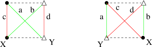
The difference from Chaudhuri et al. (2007) is that we require only a single bit at each dimension for score in the present paper. The idea that makes an inner-product based score work is that although from an individual, e.g., $Y$ ’s perspective, $\textsf{diff}(Y)$ may not be significantly positive due to the definition of our score, the sum of diffs over a pair of swapped nodes, e.g., $\textsf{diff}(X)+\textsf{diff}(Y)$ as in Figure 3, can be shown to be positive with high probability, given $K=\Omega(\ln N/\gamma)$ . Hence we prevent the sum of $\textsf{diff}(X)+\textsf{diff}(Y)$ from deviating too much from its expected value $K\gamma$ (Proposition 13), by excluding those bad node events (Definition 9), whose probability we bound in Lemma 16 and 17.

Definition 9

(Bad Node Event) Let a bad node event ${\mathcal{E}}(Z)$ be the event that $\{\textsf{diff}(Z)<\text{{\bf E}$\left[\textsf{diff}(Z)\right]$}-K\gamma/4\}$ , where $Z$ is a sample point in the mixture. Note this is an event in an individual probability space $(\Omega_{Z},\mathbb{F}_{Z},{\bf Pr}_{Z})$ , where $(\Omega_{Z},\mathbb{F}_{Z},{\bf Pr}_{Z})$ is defined over all possible outcomes of $K$ random bits for sample point $Z$ .

Note that all bad node events are mutually independent. From now on, we use $(\Omega_{i},\mathbb{F}_{i},{\bf Pr}_{i})$ to refer to $(\Omega_{Z_{i}},\mathbb{F}_{Z_{i}},{\bf Pr}_{Z_{i}})$ for the input $2N$ nodes, assuming a certain ordering.

Definition 10

(Bad Event ${\mathcal{E}}^{N}_{1}$ ) ${\mathcal{E}}^{N}_{1}$ is the same as ${\mathcal{E}}(Z_{1})\cup\ldots\cup{\mathcal{E}}(Z_{2N})$ in the product probability space $(\Omega,\mathbb{F},{\bf Pr})$ composed of distinct probability spaces $(\Omega_{1},\mathbb{F}_{1},{\bf Pr}_{1}),\ldots$ , $(\Omega_{2N},\mathbb{F}_{2N},{\bf Pr}_{2N})$ as in Definition 9. Let $\bar{\mathcal{E}}^{N}_{1}$ denote the product probability space $(\Omega,\mathbb{F},{\bf Pr})$ excluding ${{\mathcal{E}}}^{N}_{1}$ .

For each balanced cut $(S,\overline{S})$ , conditioned upon fixing a subset of random bits on all swapped nodes, as shown in Figure 2, to behave nicely in the sense of Lemma 16 and 17, we show that the conditional expectations, in the sense of Definition 20, for random variables $\textsf{diff}({\mathcal{T}},(S,\overline{S}),L)$ , $\forall L>0$ , are significantly positive, so that the perfect partition can almost always win over all other balanced cuts, in terms of the particular measure (minimum total score here), despite the large deviation events that we handle in Section 4. This idea has been explored in the proof of Chaudhuri et al. (2007) for diploid scores.

The key difference between this score and the “diploid score” (see Chaudhuri et al., 2007, Section 2.1) is that the corresponding diploid $\textsf{diff}(Y)$ is always significantly positive in expectation, i.e., $\text{{\bf E}${}_{\vec{y}\sim{\mathbf{D}}_{m}}\left[\textsf{diff}(Y)\right]$}>0$ , $\forall m=1,2$ , and thus remains so with high probability given $K=\Omega(\ln N/\gamma)$ . That is, an individual is almost always more similar to a randomly chosen peer from its population, than a randomly chosen individual from another population given a large enough $K$ based on “diploid scores”. The cost of this nice property is: two random bits from the same distribution are required at each dimension from all sample. In the present paper, we provide a similar positiveness guarantee, for a pair of scores $\textsf{diff}(X)+\textsf{diff}(Y)$ , where $\vec{x}\sim{\mathbf{D}}_{1}$ and $\vec{y}\sim{\mathbf{D}}_{2}$ , as illustrated in Figure 3. This property is due to Proposition 13, Lemma 16 and 17. We like to point out that the requirement on the input instance being balanced is due to the fact that we need pairing up two individuals such that one comes from each distribution, in order to obtain the initial expected minimality for ${\mathcal{T}}$ as defined in Proposition 18.

3.2 The Expected Difference of Two Edges

We first show that the perfect partition ${\mathcal{T}}$ has the minimum value among all balanced cuts in expectation, when summing up scores over all edges across the cut in Proposition 18. The inspiration for using an inner-product based score and pairing up $\textsf{diff}(X)$ and $\textsf{diff}(Y)$ , for $X\sim{\mathbf{D}}_{1}$ and $Y\sim{\mathbf{D}}_{2}$ , comes from Freund and Mansour (1999). We first show that the sum of expected differences over $X\sim{\mathbf{D}}_{1}$ and $Y\sim{\mathbf{D}}_{2}$ is significant.

Proposition 11

$\forall a,b=1,2,\text{{\bf E}${}_{\vec{x}\sim{\mathbf{D}}_{a},\vec{y}\sim{\mathbf{D}}_{b}}\left[<\vec{x},\vec{y}>\right]$}=<\vec{p}_{a},\vec{p}_{b}>$ .

Proof We have $\forall a,b=1,2$ , $\text{{\bf E}${}_{\vec{x}\sim{\mathbf{D}}_{a},\vec{y}\sim{\mathbf{D}}_{b}}\left[<\vec{x},\vec{y}>\right]$}=\text{{\bf E}$\left[\sum_{i=1}^{K}x^{i}y^{i}\right]$}=\sum_{i=1}^{K}\text{{\bf E}$\left[x^{i}y^{i}\right]$}=\sum_{i=1}^{K}p^{i}_{a}p^{i}_{b}=<\vec{p}_{a},\vec{p}_{b}>.$

Proposition 12

Let $X$ be a sample point from ${\mathbf{D}}_{1}$ and $Y$ be a point from ${\mathbf{D}}_{2}$ , $\textsf{diff}(X)=\sum_{i=1}^{K}x^{i}(p^{i}_{1}-p^{i}_{2}),$ and $\textsf{diff}(Y)=\sum_{i=1}^{K}y^{i}(p^{i}_{2}-p^{i}_{1})$ .

Proposition 13

(Freund and Mansour, 1999) $\text{{\bf E}${}_{\vec{x}\sim\vec{p}_{1}}\left[\textsf{diff}(X)\right]$}+\text{{\bf E}${}_{\vec{y}\sim\vec{p}_{2}}\left[\textsf{diff}(Y)\right]$}=\left\lVert\vec{p}_{1}-\vec{p}_{2}\right\rVert_{2}^{2}=K\gamma$ .

Proof By Proposition 12, $\text{{\bf E}${}_{\vec{x}\sim\vec{p}_{1}}\left[\textsf{diff}(X)\right]$}+\text{{\bf E}${}_{\vec{y}\sim\vec{p}_{2}}\left[\textsf{diff}(Y)\right]$}=\sum_{i=1}^{K}p^{i}_{1}(p^{i}_{1}-p^{i}_{2})+\sum_{i=1}^{K}p^{i}_{2}(p^{i}_{2}-p^{i}_{1})=<\vec{p}_{1},\vec{p}_{1}-\vec{p}_{2}>+<\vec{p}_{2},\vec{p}_{2}-\vec{p}_{1}>=K\gamma.$

Before we proceed, we first state the following theorem and its corollary on Hoeffding Bounds.

Theorem 14

(Hoeffding, 1963) If $X_{1},X_{2},\ldots,X_{K}$ are independent and $a_{i}\leq X_{i}\leq b_{i},\forall i=1,2,\ldots,K$ , and if $\bar{X}=(X_{1}+\ldots+X_{K})/K$ and $\mu=\text{{\bf E}$\left[\bar{X}\right]$}$ , then for $t>0$ , $\text{{\bf Pr}$\left[\bar{X}-\mu\geq t\right]$}\leq e^{-2K^{2}t^{2}/\sum_{i=1}^{K}(b_{i}-a_{i})^{2}}.$

Corollary 15

(Hoeffding, 1963) If $Y_{1},\ldots,Y_{n}$ , $Z_{1},\ldots,Z_{m}$ are independent random variables with values in the interval $[a,b]$ , and if $\bar{Y}=(Y_{1}+\ldots+Y_{m})/m$ , $\bar{Z}=(Z_{1}+\ldots+Z_{n})/n$ , then for $t>0$ ,

\text{{\bf Pr}$\left[\bar{Y}-\bar{Z}-(\text{{\bf E}$\left[\bar{Y}\right]$}-\text{{\bf E}$\left[\bar{Z}\right]$})\geq t\right]$}\leq e^{-2t^{2}/(m^{-1}+n^{-1})(b-a)^{2}}.

Let us denote w.l.o.g. $\eta=\text{{\bf E}${}_{\vec{x}\sim\vec{p}_{1}}\left[\textsf{diff}(X)\right]$}\geq K\gamma/2$ , and thus $\text{{\bf E}${}_{\vec{y}\sim\vec{p}_{2}}\left[\textsf{diff}(X)\right]$}=K\gamma-\eta$ , and show the following two lemmas.

Lemma 16

Given that $K\geq\frac{8\ln{1/\tau}}{\gamma}$ , $\text{{\bf Pr}${}_{X}\left[\textsf{diff}(X)<\eta-K\gamma/4\right]$}<\tau$ .

Proof Let us define $\gamma_{k}=(p_{1}^{k}-p_{2}^{k})^{2},\forall k=1,\ldots,K$ . Given that $x^{1},\ldots,x^{K}$ are independent Bernoulli random variables and $(p^{k}_{1}-p^{k}_{2})x^{k}$ is either in $[0,\sqrt{\gamma_{k}}]$ or $[-\sqrt{\gamma_{k}},0]$ , $\forall k=1,\ldots,K$ , we apply Hoeffding bound as in Theorem 14 with $t=K\gamma/4K=\gamma/4$ :

	Pr ${}_{X}\left[-\sum_{k=1}^{K}(p^{k}_{1}-p^{k}_{2})x^{k}+\eta\geq K\gamma/4\right]$	$\displaystyle=$	Pr ${}_{X}\left[\sum_{k=1}^{K}(p^{k}_{1}-p^{k}_{2})x^{k}-\eta\leq-K\gamma/4\right]$
		$\displaystyle\leq$	$\displaystyle e^{-2K^{2}(\gamma/4)^{2}/\sum_{k=1}^{K}{(\sqrt{\gamma_{k}})^{2}}}\leq\tau.$

Thus we have that $\text{{\bf Pr}${}_{X}\left[\sum_{k=1}^{K}(p^{k}_{1}-p^{k}_{2})x^{k}\geq\eta-K\gamma/4\right]$}\geq 1-\tau$ .

Lemma 17

Given that $K\geq\frac{8\ln{1/\tau}}{\gamma}$ , $\text{{\bf Pr}${}_{Y}\left[\textsf{diff}(Y)<(K\gamma-\eta)-K\gamma/4\right]$}<\tau$ .

Proof Similar to proof of Lemma 16, we have $\text{{\bf Pr}${}_{Y}\left[\sum_{k=1}^{K}(p^{k}_{2}-p^{k}_{1})y^{i}-(K\gamma-\eta)\leq-K\gamma/4\right]$}\leq\tau$ , where $K\gamma-\eta=\text{{\bf E}${}_{\vec{y}\sim\vec{p}_{2}}\left[\textsf{diff}(Y)\right]$}$ . Hence $[\text{{\bf Pr}${}_{Y}\left[\sum_{k=1}^{K}(p^{k}_{2}-p^{k}_{1})y^{i}\geq(K\gamma-\eta)-K\gamma/4\right]$}\geq 1-\tau.$

In particular, combining $(\ref{eq:exp-diff})$ and Proposition 13, we have the following.

Proposition 18

$\text{{\bf E}$\left[\textsf{diff}({\mathcal{T}},(S,\overline{S}),L)\right]$}=(N-L)LK\gamma$ .

Proof By Definition 5, we have

$\displaystyle\textsf{diff}(X)=\text{{\bf E}${}_{\vec{x^{\prime}}\sim\vec{p}_{1}}\left[\textsf{score}(X,X^{\prime})\right]$}-\text{{\bf E}${}_{\vec{y^{\prime}}\sim\vec{p}_{2}}\left[\textsf{score}(X,Y^{\prime})\right]$}$
	$\displaystyle=$	$\displaystyle\text{{\bf E}${}_{\vec{x^{\prime}}\sim\vec{p}_{1}}\left[<\vec{x},\vec{x^{\prime}}>\right]$}-\text{{\bf E}${}_{\vec{y^{\prime}}\sim\vec{p}_{2}}\left[<\vec{x},\vec{y^{\prime}}>\right]$}=<\vec{x},\vec{p}_{1}-\vec{p}_{2}>=\sum_{i=1}^{K}x^{i}(p^{i}_{1}-p^{i}_{2}),$
$\displaystyle\textsf{diff}(Y)=\text{{\bf E}${}_{\vec{y^{\prime}}\sim\vec{p}_{2}}\left[\textsf{score}(Y,Y^{\prime})\right]$}-\text{{\bf E}${}_{\vec{x^{\prime}}\sim\vec{p}_{1}}\left[\textsf{score}(Y,X^{\prime})\right]$}$
	$\displaystyle=$	$\displaystyle\text{{\bf E}${}_{\vec{y^{\prime}}\sim\vec{p}_{2}}\left[<\vec{y},\vec{y^{\prime}}>\right]$}-\text{{\bf E}${}_{\vec{x^{\prime}}\sim\vec{p}_{1}}\left[<\vec{y},\vec{x^{\prime}}>\right]$}=<\vec{y},\vec{p}_{2}-\vec{p}_{1}>=\sum_{i=1}^{K}y^{i}(p^{i}_{2}-p^{i}_{1}).$

Given such a positiveness guarantee on the conditional expectations of $\textsf{diff}({\mathcal{T}},(S,\overline{S}),L)$ described above, the rest of the proof focus on bounding large deviation events; a sketch of the key ideas has appeared in Chaudhuri et al. (2007, Section 3), based on “diploid scores”. We need to show that, with high probability, all of $O(2^{n})$ random variables, in the form of $\textsf{diff}({\mathcal{T}},(S,\overline{S}),L)$ , stay positive all simultaneously, given enough number of features and total number of random bits. We describe the important ideas of this proof in next three sections, which contain key lemmas for each step; more proofs are contained in the appendix for completeness of presentation.

4 Proof Techniques for Concentration

We first introduce some notation regarding the sample probability space $(\Omega,\mathbb{F},{\bf Pr})$ . The set $\Omega$ is the set of all possible outcomes for $2NK$ random bits, where we denote each bit as $b^{k}_{j}$ for a point $j$ at dimension $k$ . The $\sigma$ -field $\mathbb{F}$ of events is the set $\Sigma(\Omega)$ of all subsets of $\Omega$ ; and the probability measure ${\bf Pr}$ is based on the product of probabilities of each random bit $b^{k}_{j},\forall k,j$ , corresponding to Bernoulli( $p^{k}_{a}$ ), where $a\in\{1,2\}$ depends on the population of origin for individual $j$ . Formally,

Definition 19

The elementary events in the underlying sample space $(\Omega,\mathbb{F},{\bf Pr})$ are all possible $2^{2NK}$ choices of $D=2NK$ bits. For $0\leq i\leq D$ and $w\in\{0,1\}^{i}$ , let $B_{w}$ denote the event that the first $i$ bits equal to the bit string $w$ . Let $\mathbb{F}_{i}$ be the $\sigma$ -field generated by the partition of $\Omega$ into blocks $B_{w}$ , for $w\in\{0,1\}^{i}$ . Then the sequence $\mathbb{F}_{0},\ldots,\mathbb{F}_{D}$ forms a filter. In the $\sigma$ -field $\mathbb{F}_{i}$ , the only valid events are the ones that depend on the values of the first $i$ bits, and all such events are valid within.

The events that we define next and their interactions are shown in Figure 5. We show that, with high probability, all of the $O(2^{2N})$ random variables $\textsf{diff}({\mathcal{T}},(S,\overline{S}),L)$ , as in (2), one corresponding to each balanced $(S,\bar{S})$ , are positive. We initially confine ourselves into a good subspace $\bar{{\mathcal{E}}}^{N}_{1}$ by excluding any bad node event (Definition 9). This subspace has the nice property in the sense of Theorem 23. We then use union bound to bound the probability of any bad score event in this subspace, where a single bad score event occurs when $\textsf{diff}({\mathcal{T}},(S,\overline{S}),L)\leq 0$ for a particular balanced $(S,\bar{S})$ . We use the bounded differences method to bound probabilities of such events.

Each time we examine $\textsf{diff}({\mathcal{T}},(S,\overline{S}),L)$ for a particular balanced $(S,\bar{S})$ , we let vector $(H_{1},\ldots,H_{2KN})$ record the entire history of random bits, where $(H_{1},\ldots,H_{2KL})$ record the partial history of bits on the $2L$ swapped nodes corresponding to $(S,\bar{S})$ . Let $\ell=2KL$ be a positive integer. We denote this $2KL$ -history with $\underline{H}^{(\ell)}$ . For a balanced $(S,\bar{S})$ , let $\underline{h}$ be a fixed possible $\ell$ -history: $\underline{h}=\{\tilde{U_{1}},\ldots,\tilde{U_{L}},\tilde{V_{1}},\ldots,\tilde{V_{L}}\}$ denotes a vector of $2KL$ random bits on $2L$ swapped nodes as shown in Figure 2, where $\tilde{X}$ is the outcome of a particular point $X$ in our sample. Let $\Omega_{\underline{h}}$ denote that event that we observe this particular $2KL$ -history: $\Omega_{\underline{h}}=\{\pi\in\Omega:H^{(\ell)}(\pi)=\underline{h}\}$ . Given that $\Omega_{\underline{h}}$ occurs, we are concerned about the following probability space $(\Omega_{\underline{h}},\Sigma(\Omega_{\underline{h}}),{\bf Pr}_{\underline{h}})$ , we have the following definition and proposition.

Definition 20

$\text{{\bf E}${}_{\underline{h}}\left[\textsf{diff}({\mathcal{T}},(S,\overline{S}),L)\right]$}=\text{{\bf E}$\left[\textsf{diff}({\mathcal{T}},(S,\overline{S}),L)|\mathbb{F}_{2KL}\right]$}$ is the expected value of $\textsf{diff}({\mathcal{T}},(S,\overline{S}),L)$ conditioned on an event $\underline{h}\in\mathbb{F}_{2KL}$ . This conditional expectation E $\left[\textsf{diff}({\mathcal{T}},(S,\overline{S}),L)|\mathbb{F}_{2KL}\right]$ is a random variable that can be viewed as a function into ${\mathbb{R}}$ from the blocks in the partition of $\mathbb{F}_{2KL}$ .

Hence E ${}_{\underline{h}}\left[\textsf{diff}({\mathcal{T}},(S,\overline{S}),L)\right]$ is an evaluation at a particular outcome $\underline{h}\in\mathbb{F}_{2KL}$ .

Proposition 21

For a particular outcome $\underline{h}\in\mathbb{F}_{2KL}$ , $\text{{\bf E}${}_{\underline{h}}\left[\textsf{diff}({\mathcal{T}},(S,\overline{S}),L)\right]$}=(N-L)\sum_{j=1}^{L}\textsf{diff}(\tilde{U}_{j})+(N-L)\sum_{j=1}^{L}\textsf{diff}(\tilde{V}_{j})=(N-L)\sum_{j=1}^{L}\sum_{k=1}^{K}(p^{k}_{1}-p^{k}_{2})(\tilde{u}^{k}_{j}-\tilde{v}^{k}_{j}).$

Our starting point for using the bounded differences method to bound a single bad score event over $(S,\bar{S})$ is when we have revealed the $2KL$ bits and obtained a $2KL$ -history $\underline{h}$ in $\bar{{\mathcal{E}}}^{N}_{1}$ . Given a fixed history $\underline{h}$ , we call the remaining $2K(N-L)$ bits on unswapped nodes as the $2K(N-L)$ -future. Let $\bar{f}=(H_{2KL+1},\ldots,H_{2KN})$ be a fixed possible $2K(N-L)$ -future. For simplicity of analysis, given $\underline{h}$ , we first expand the confined subspace $\bar{{\mathcal{E}}}^{N}_{1}$ by dropping constraints on the $2(N-L)$ unswapped nodes.

In this expanded subspace, we only require the first $2L$ swapped nodes to be good nodes, a condition that we denote with $\bar{{\mathcal{E}}}^{L}_{1}(S,\bar{S})$ , while leaving bits on the $2(N-L)$ unswapped nodes unconstrained; that is, these nodes can be bad nodes. Thus $(\Omega_{\underline{h}},\Sigma(\Omega_{\underline{h}}),{\bf Pr}_{\underline{h}})$ corresponds to the expanded subspace of $\bar{{\mathcal{E}}}^{N}_{1}$ given $\underline{h}$ , where we can apply the bounded differences method to analyze probability for $\{\textsf{diff}({\mathcal{T}},(S,\overline{S}),L)\leq 0\}$ in a clean manner applying Azuma’s Inequality as in Lemma 36. In fact, our starting point of the bounded differences analysis is E ${}_{\underline{h}}\left[\textsf{diff}({\mathcal{T}},(S,\overline{S}),L)\right]$ , where $\underline{h}$ is a fixed possible $2KL$ -history on the $2L$ swapped nodes for $(S,\bar{S})$ , subject to $\underline{h}\in\bar{{\mathcal{E}}}^{L}_{1}(S,\bar{S})$ :

Definition 22

${\mathcal{E}}^{L}_{1}(S,\bar{S})$ is the same as ${\mathcal{E}}(U_{1})\cup\ldots\cup{\mathcal{E}}(U_{L})\cup{\mathcal{E}}(V_{1})\cup\ldots\cup{\mathcal{E}}(V_{L})$ in the product probability space composed of distinct probability spaces defined over nodes $U_{1},\ldots,U_{L},V_{1},\ldots,V_{L}$ as in Definition 9.

This immediately indicates that the conditional expected value $\text{{\bf E}${}_{\underline{h}}\left[\textsf{diff}({\mathcal{T}},(S,\overline{S}),L)\right]$}\geq(N-L)LK\gamma/2$ , which is our “advantageous base point” given that $\Omega_{\underline{h}}$ occurs. The proof of the following theorem appears in Section 5.

Theorem 23

Give that all points are drawn from $\bar{{\mathcal{E}}}^{N}_{1}$ , the probability space $(\Omega,\mathbb{F},{\bf Pr})$ excluding ${{\mathcal{E}}}^{N}_{1}$ , we have $\forall$ balanced $(S,\bar{S})$ , where $\underline{h}$ is a particular $2KL$ -history corresponding to the $2L$ swapped nodes specified over $(S,\bar{S})$ with respect to ${\mathcal{T}}$ ,

\displaystyle\text{{\bf E}${}_{\underline{h}}\left[\textsf{diff}({\mathcal{T}},(S,\overline{S}),L)\right]$}\geq(N-L)LK\gamma/2,

(4)

where the conditional expectation is over each of the individually expanded probability space $(\Omega_{\underline{h}},\Sigma(\Omega_{\underline{h}}),{\bf Pr}_{\underline{h}})$ given $\underline{h}\in\bar{{\mathcal{E}}}^{L}_{1}$ , where ${\mathcal{E}}^{L}_{1}$ is defined in Definition 22. This statement remains true after we require that $\underline{h}\in\bar{{\mathcal{E}}}^{L}_{2}$ in addition, where ${\mathcal{E}}^{L}_{2}$ is defined in Definition 26.

Now as we reveal one by one the future $2K(N-L)$ random bits, the conditional expected values $\text{{\bf E}${}_{\underline{h}}\left[\textsf{diff}({\mathcal{T}},(S,\overline{S}),L)|\underline{H}^{(\ell^{\prime})}\right]$},\forall\ell^{\prime}\geq 2KL$ form a martingale that is amenable to the bounded differences analysis as shown in Theorem 37 in Section 6. However, in order to obtain a concentration bound as tight as that in Theorem 37, we need to exclude one more event ${\mathcal{E}}^{L}_{2}$ as in Definition 26, from the $2KL$ -history $\underline{h}$ , while examining a balanced $(S,\bar{S})$ . We first give some definitions regarding ${\mathcal{E}}^{L}_{2}$ . Nodes are shown in Figure 2.

Definition 24

Given vectors $\vec{u_{1}},\ldots,\vec{u_{L}}$ and $\vec{v_{1}},\ldots,\vec{v_{L}}$ , where $u^{k}_{j},v^{k}_{j}$ are the $k^{th}$ bit of $U_{j}$ and $V_{j}$ respectively, $f_{2}^{k}(\underline{h})=\sum_{j=1}^{L}u^{k}_{j}-\sum_{j=1}^{L}v^{k}_{j}.$

Definition 25

(Deviation Values) $\forall k=1,\ldots,K$ , let $t_{k}\sqrt{L}$ be the exact deviation on $f_{2}^{k}(\underline{h})$ , i.e., $f^{k}_{2}(\underline{h})-\text{{\bf E}$\left[f^{k}_{2}(\underline{h})\right]$}=t_{k}\sqrt{L},\forall k$ .

Definition 26

(Bad Deviation Event ${\mathcal{E}}^{L}_{2}$ ) In probability space $(\Omega,\mathbb{F},{\bf Pr})$ , given a balanced $(S,\bar{S})$ and its corresponding $2KL$ -history $\underline{h}$ , ${\mathcal{E}}^{L}_{2}$ is the event such that the set of random variables $t_{1},\ldots,t_{k}$ regarding $2KL$ random bits recorded in $\underline{h}$ , as defined in Definition 25, are simultaneously large and satisfy $\sum_{k=1}^{K}{t}^{2}_{k}\geq\Delta=8N\ln 2+4K\ln 2(\log\log N+1)+3\ln N/2$ .

Using Definition 26 and 25, we immediately have the following lemma.

Lemma 27

Given that $\underline{h}\in\bar{{\mathcal{E}}}_{2}^{L}$ , we have $\forall k$ ,

\displaystyle\left|f^{k}_{2}(\underline{h})\right|\leq\left|\text{{\bf E}$\left[f^{k}_{2}(\underline{h})\right]$}\right|+\left|t_{k}\sqrt{L}\right|,

and $\sum_{k=1}^{K}{t}^{2}_{k}\leq\Delta$ , where $t_{k}$ is in Definition 25, and ${\mathcal{E}}^{L}_{2}$ is in Definition 26.

Proof By definition of $t_{k},\forall k$ , we have that $f^{k}_{2}(\underline{h})=\text{{\bf E}$\left[f^{k}_{2}(\underline{h})\right]$}+t_{k}\sqrt{L}$ , where $t_{k}\in[\frac{-L-\text{{\bf E}$\left[f^{k}_{2}(\underline{h})\right]$}}{\sqrt{L}},\frac{L-\text{{\bf E}$\left[f^{k}_{2}(\underline{h})\right]$}}{\sqrt{L}}]$ . Thus the lemma holds given that $\underline{h}\in\bar{{\mathcal{E}}}_{2}^{L}$ .

Excluding ${\mathcal{E}}^{L}_{2}$ from $\underline{h}$ is crucial in bounding the difference that each of the $2(N-L)K$ -future random bits causes when we work in probability space $(\Omega_{\underline{h}},\Sigma(\Omega_{\underline{h}}),{\bf Pr}_{\underline{h}})$ , where the difference refers to

\left|\text{{\bf E}${}_{\underline{h}}\left[\textsf{diff}({\mathcal{T}},(S,\bar{S}),L)|\underline{H}^{(\ell^{\prime})}\right]$}-\text{{\bf E}${}_{\underline{h}}\left[\textsf{diff}({\mathcal{T}},(S,\overline{S}),L)|\underline{H}^{(\ell^{\prime}-1)}\right]$}\right|,

where $2KN\geq\ell^{\prime}>2KL$ depends on the bit, such that the square sum of all these differences is not too big as in Lemma 27. This is illustrated in the second graph in Figure 2. This allows us to bound the probability on a bad score event, i.e., $\textsf{diff}({\mathcal{T}},(S,\overline{S}),L)\leq 0,$ using Azuma’s inequality in probability space $(\Omega_{\underline{h}},\Sigma(\Omega_{\underline{h}}),{\bf Pr}_{\underline{h}})$ as in Section 6. The proof of the following lemma is rather long and shown in Section A.1.

Lemma 28

Let $\underline{h}$ be the specific $2KL$ -history that we record for a balanced cut $(S,\bar{S})$ such that $\underline{h}\in\bar{{\mathcal{E}}}^{L}_{1}\cap\bar{{\mathcal{E}}}^{L}_{2}$ . Let $\rho^{L}_{3}=\frac{2}{N^{4L}}$ . Then for $K=\Omega(\frac{\ln N}{\gamma})$ and $KN=\Omega(\frac{\ln N\log\log N}{\gamma^{2}})$ , for all $N\geq 4$ ,

\text{{\bf Pr}$\left[\textsf{diff}({\mathcal{T}},(S,\overline{S}),L)\leq 0|\underline{h}\in\bar{{\mathcal{E}}}^{L}_{2}\cap\bar{{\mathcal{E}}}^{L}_{1},\bar{f}\mbox{ at random}\right]$}\leq\rho^{L}_{3}.

Eventually we compute the probability of events $\{\textsf{diff}({\mathcal{T}},(S,\overline{S}),L)\leq 0\}$ in $\bar{{\mathcal{E}}}^{N}_{1}$ for all balanced $(S,\overline{S})$ in Section 7.

5 Proof of Theorem 23

This section is dedicated to prove Theorem 23. We first give another definition.

Definition 29

${\mathcal{E}}^{N-L}_{1}(S,\bar{S})$ is the same as ${\mathcal{E}}(X_{1})\cup\ldots\cup{\mathcal{E}}(X_{N-L})\cup{\mathcal{E}}(Y_{1})\cup\ldots\cup{\mathcal{E}}(Y_{N-L})$ in the product probability space composed of distinct probability spaces defined over nodes $X_{1},\ldots,X_{N-L}$ and $Y_{1},\ldots,Y_{N-L}$ as in Definition 9.

Hence $\bar{{\mathcal{E}}}^{L}_{1}$ and $\bar{{\mathcal{E}}}^{N-L}_{1}$ imply that no bad node event happens in the appropriate product spaces thus defined. We omit $(S,\bar{S})$ from ${\mathcal{E}}^{L}_{1}(S,\bar{S})$ and ${\mathcal{E}}^{N-L}_{1}(S,\bar{S})$ when it is clear from the context. Given a balanced cut $(S,\bar{S})$ , $\underline{h}$ records a history on the $2KL$ bits on swapped nodes $U_{1},\ldots,U_{L},V_{1},\ldots,V_{L}$ .

Proposition 30

Given all nodes are drawn from $\bar{{\mathcal{E}}}^{N}_{1}$ , for any balanced cut $(S,\bar{S})$ and its particular $2KL$ -history $\underline{h}$ that we record must satisfy the following: $\underline{h}\in\bar{{\mathcal{E}}}^{L}_{1}(S,\bar{S})$ .

Proof Given $\bar{{\mathcal{E}}}^{N}_{1}$ , we know that for all nodes $Z_{1},\ldots,Z_{2N}$ ,

\displaystyle\textsf{diff}(Z_{i})\geq\text{{\bf E}$\left[\textsf{diff}(Z_{i})\right]$}-K\gamma/4,

(5)

simultaneously in the product probability space $(\Omega,\mathbb{F},{\bf Pr})$ , where $\textsf{diff}(Z_{i})$ is a random variable solely determined by node $Z_{i}$ ’s bit vector. In particular, for each balanced $(S,\bar{S})$ , we focus on the product probability space that is composed of distinct probability spaces defined over swapped nodes $U_{1},\ldots,U_{L},V_{1},\ldots,V_{L}$ as in Definition 22. After we reveal these $2L$ bit vectors on $U_{j},V_{j},\forall j=1,\ldots,L$ , by (5),

	$\displaystyle\textsf{diff}(U_{j})$	$\displaystyle\geq$	$\displaystyle\text{{\bf E}$\left[\textsf{diff}(U_{j})\right]$}-K\gamma/4,\forall j=1,\ldots,L,$		(6)
	$\displaystyle\textsf{diff}(V_{j})$	$\displaystyle\geq$	$\displaystyle\text{{\bf E}$\left[\textsf{diff}(V_{j})\right]$}-K\gamma/4,\forall j=1,\ldots,L.$		(7)

Thus we have $\underline{h}\in\bar{{\mathcal{E}}}^{L}_{1}(S,\bar{S})$ .

Definition 31

We use $\bar{f}$ to denote the future of the $2(N-L)K$ random bits that we are going to reveal for the unswapped nodes on a given balanced cut $(S,\bar{S})$ . Recall that once we are fixed to the probability space such that ${\mathcal{E}}^{N}_{1}$ does not happen, we know that both $\underline{h}$ and $\bar{f}$ are confined; the following two notation are equivalent:

	$\displaystyle(\underline{h}\in\bar{{\mathcal{E}}}^{L}_{1}(S,\bar{S}))$	$\displaystyle\cap$	$\displaystyle(\bar{f}\in\bar{{\mathcal{E}}}^{N-L}_{1}(S,\bar{S})),$
	$\displaystyle(\underline{h},\bar{f})$	$\displaystyle\in$	$\displaystyle\bar{{\mathcal{E}}}^{N}_{1}.$

Remark 32

Another way of seeing $\bar{{\mathcal{E}}}^{L}_{1}(S,\bar{S})$ (with respect to a particular balanced cut $(S,\bar{S})$ ) is to view it as an event in the simple probability space $(\Omega,\mathbb{F},{\bf Pr})$ , such that we put constraints only on the specific $2L$ swapped nodes defined on $(S,\bar{S})$ while leaving the $\bar{f}$ at random. Hence we have $\bar{{\mathcal{E}}}^{N}_{1}\subset\bar{{\mathcal{E}}}^{L}_{1}(S,\bar{S})$ in $(\Omega,\mathbb{F},{\bf Pr})$ .

We leave this confined space given $\bar{{\mathcal{E}}}^{N}_{1}$ for now and explore the following expanded subspace, where we require $\underline{h}\in\bar{{\mathcal{E}}}^{L}_{1}$ while leaving the future $\bar{f}$ at random. $(\Omega_{\underline{h}},\Sigma(\Omega_{\underline{h}}),{\bf Pr}_{\underline{h}})$ corresponds to this expanded subspace, where $\underline{h}\in\bar{{\mathcal{E}}}^{L}_{1}$ . This immediately implies the following lemma.

Lemma 33

For a balanced cut $(S,\bar{S})$ , given a particular $2KL$ -history $\underline{h}\in F_{2KL}$ on the $2L$ swapped nodes such that $\underline{h}\in\bar{{\mathcal{E}}}^{L}_{1}$ ,

\displaystyle\text{{\bf E}${}_{\underline{h}}\left[\textsf{diff}({\mathcal{T}},(S,\overline{S}),L)|\underline{h}\in\bar{{\mathcal{E}}}^{L}_{1},\bar{f}\mbox{ at random}\right]$}\geq L(N-L)K\gamma/2,

(8)

where expectation is over all possible outcomes of the $2(N-L)K$ random bits in $\bar{f}$ in probability space $(\Omega_{\underline{h}},\Sigma(\Omega_{\underline{h}}),{\bf Pr}_{\underline{h}})$ .

Proof For a balanced cut $(S,\bar{S})$ , given $\underline{h}\in\bar{{\mathcal{E}}}^{L}_{1}$ , where $\underline{h}$ records $2KL$ bits over swapped nodes $U_{j},V_{j},\forall j=1,\ldots,L$ , by Definition 9,

	$\displaystyle\textsf{diff}(U_{j})$	$\displaystyle\geq$	$\displaystyle\text{{\bf E}$\left[\textsf{diff}(U_{j})\right]$}-K\gamma/4,\forall j=1,\ldots,L,$		(9)
	$\displaystyle\textsf{diff}(V_{j})$	$\displaystyle\geq$	$\displaystyle\text{{\bf E}$\left[\textsf{diff}(V_{j})\right]$}-K\gamma/4,\forall j=1,\ldots,L,$		(10)

and hence $\textsf{diff}(U_{j})+\textsf{diff}(V_{j})\geq K\gamma/2,\forall j=1,\ldots,L$ by Proposition 13. Thus, in $(\Omega_{\underline{h}},\Sigma(\Omega_{\underline{h}}),{\bf Pr}_{\underline{h}})$ , where $\bar{f}$ is at random and $\underline{h}\in\bar{{\mathcal{E}}}^{L}_{1}$ , we have from Proposition 21,

	E ${}_{\underline{h}}\left[\textsf{diff}({\mathcal{T}},(S,\bar{S}),L)\right]$	$\displaystyle=$	$\displaystyle(N-L)\sum_{j=1}^{L}\textsf{diff}(U_{j})+(N-L)\sum_{j=1}^{L}\textsf{diff}(V_{j})$
		$\displaystyle\geq$	$\displaystyle(N-L)\sum_{j=1}^{L}(\textsf{diff}(U_{j})+\textsf{diff}(V_{j}))\geq(N-L)LK\gamma/2.$

Recall that $\bar{{\mathcal{E}}}^{L}_{2}$ is the event that no simultaneously large deviation happens across $2L$ individuals over their $2KL$ random bits.

Corollary 34

Given that $\underline{h}\in\bar{{\mathcal{E}}}^{L}_{1}\cap\bar{{\mathcal{E}}}^{L}_{2}$ , and $\bar{f}$ is at random:

\displaystyle\text{{\bf E}${}_{\underline{h}}\left[\textsf{diff}({\mathcal{T}},(S,\overline{S}),L)|\underline{h}\in\bar{{\mathcal{E}}}^{L}_{1}\cap\bar{{\mathcal{E}}}^{L}_{2},\bar{f}\mbox{ at random}\right]$}\geq L(N-L)K\gamma/2,

(11)

which holds so long as $\underline{h}\in\bar{{\mathcal{E}}}^{L}_{1}$ .

We next bound E ${}_{\underline{h}}\left[\textsf{diff}({\mathcal{T}},(S,\overline{S}),L)\right]$ for all balanced $(S,\bar{S})$ , where $\underline{h}$ is confined in $\bar{{\mathcal{E}}}^{N}_{1}$ and $\bar{{\mathcal{E}}}^{L}_{2}$ . We now prove Theorem 23.

Proof of Theorem 23. By Proposition 30, for each balanced cut $(S,\bar{S})$ , we have

\displaystyle\underline{h}\in\bar{{\mathcal{E}}}^{L}_{1}(S,\bar{S}).

(12)

Now apply Corollary 34, given that $\underline{h}\in\bar{{\mathcal{E}}}^{L}_{1}(S,\bar{S})\cap\bar{{\mathcal{E}}}^{L}_{2}$ , we immediately have the theorem.

Remark 35

$\textsf{diff}(Z)$ is determined by node $Z$ ’s bit pattern, which is the same when we observe it from every balanced cut, where it acts as a swapped node. Hence although we do have $O(2^{n})$ balanced cuts, E ${}_{\underline{h}}\left[\textsf{diff}({\mathcal{T}},(S,\bar{S}),L)\right]$ for all balanced cuts are just determined by the $2N$ random variables $\textsf{diff}(Z_{1}),\ldots,$ $\textsf{diff}(Z_{2N})$ , each of which is determined by the bit vector of an individual in our sample.

6 Bounded Differences

In order to show Lemma 28 (actual proof see Section A.1), we prove Theorem 37 in this section, where we bound the deviation of random variable $\textsf{diff}({\mathcal{T}},(S,\overline{S}),L)$ for a particular balanced cut $(S,\bar{S})$ . Recall that we let bit vector $(H_{1},\ldots,H_{2KN})$ record the entire history of random bits that we see, where $(H_{1},\ldots,H_{2KL})$ record the $2KL$ -history $\underline{H}^{(\ell)}$ on $2L$ swapped nodes. First it is convenient to introduce some more notation: For $\ell^{\prime}\geq 2KL$ , we begin to reveal the random bits on unswapped nodes in $(S,\bar{S})$ . The random variable E ${}_{\underline{h}}\left[\textsf{diff}({\mathcal{T}},(S,\overline{S}),L)|\underline{H}^{(\ell^{\prime})}\right]$ depends on the random extension $\underline{H}^{(\ell^{\prime})}$ of $\underline{h}$ observed. By definition $\text{{\bf E}${}_{\underline{h}}\left[\textsf{diff}({\mathcal{T}},(S,\overline{S}),L)|\underline{H}^{(\ell^{\prime})}\right]$}(\pi)=\text{{\bf E}${}_{\underline{h}}\left[\textsf{diff}({\mathcal{T}},(S,\overline{S}),L)|\underline{H}^{(\ell^{\prime})}=\underline{h}^{\prime}\right]$}$ for $\pi\in\Omega_{\underline{h}}$ , where $\underline{h}^{\prime}=\underline{H}^{(\ell^{\prime})}(\pi)$ ; another notation for this is E ${}_{\underline{h}}\left[\textsf{diff}({\mathcal{T}},(S,\overline{S}),L)|\mathbb{F}\right]$ where $\mathbb{F}$ is the $\sigma$ -field generated by $\underline{H}^{(\ell^{\prime})}$ restricted to $\Omega_{\underline{h}}$ . To prove the theorem, we introduce the following.

Lemma 36

(Azuma’s Inequality) Let $Z_{0},Z_{1},\ldots,Z_{m}=f$ be a martingale on some probability space, and suppose that $|Z_{i}-Z_{i-1}|\leq c_{i}$ , $\forall i=1,2,\ldots,m$ , then

\text{{\bf Pr}$\left[|f-\text{{\bf E}$\left[f\right]$}|\geq t\right]$}\leq 2e^{-t^{2}/2\sigma^{2}},

where $\sigma^{2}=\sum_{i=1}^{m}c_{i}^{2}$ .

We are now ready to use bounded differences approach in $(\Omega_{\underline{h}},\Sigma(\Omega_{\underline{h}}),{\bf Pr}_{\underline{h}})$ and prove Theorem 37.

Theorem 37

Let $\underline{h}$ be a possible $2KL$ -history that we record for a balanced cut $(S,\bar{S})$ such that $\underline{h}\in\bar{{\mathcal{E}}}^{L}_{2}\cap\bar{{\mathcal{E}}}^{L}_{1}$ . Then, for $t>0$ , in probability space $(\Omega_{\underline{h}},\Sigma(\Omega_{\underline{h}}),{\bf Pr}_{\underline{h}})$ , where all future $2(N-L)K$ random bits $\bar{f}$ are completely at random,

\text{{\bf Pr}${}_{\underline{h}}\left[|\text{{\bf E}${}_{\underline{h}}\left[\textsf{diff}({\mathcal{T}},(S,\bar{S}),L)|\underline{H}^{2KN}\right]$}-\text{{\bf E}${}_{\underline{h}}\left[\textsf{diff}({\mathcal{T}},(S,\bar{S}),L)\right]$}|\geq t\right]$}\leq 2e^{-t^{2}/2\sigma^{2}},

where $\sigma^{2}\leq 4(N-L)L^{2}(K\gamma)+4(N-L)L\Delta$ , for all balanced $(S,\bar{S})$ with $0<L\leq N/2$ swapped nodes.

Proof We shall set up things to use Lemma 36. We work in probability space $(\Omega_{\underline{h}},\Sigma(\Omega_{\underline{h}}),{\bf Pr}_{\underline{h}})$ . We start to reveal the $2K(N-L)$ bits on unswapped nodes that are chosen independently at random, and rely on $2L$ swapped nodes having a good history $\underline{h}$ , given that $\underline{h}\in\bar{{\mathcal{E}}}^{L}_{2}\cap\bar{{\mathcal{E}}}^{L}_{1}$ .

Given the $\sigma$ -field $(\Omega_{\underline{h}},\Sigma(\Omega_{\underline{h}}))$ , with $\Sigma(\Omega_{\underline{h}})=2^{\Omega_{\underline{h}}}$ , let us first define a filter ${\mathbf{F}}$ . Given independent random bits $H_{2KL+1},\ldots,H_{2KN}$ , the filter is defined by letting $\mathbb{F}_{i},\forall i=1,\ldots,m$ , where $m=2K(N-L)$ , be the $\sigma$ -field generated by histories $\underline{H}^{(2KL+1)},\ldots,\underline{H}^{(2KL+i)}$ . We thus obtain a natural ${\mathbf{F}}$ :

\displaystyle\{\emptyset,\Omega_{\underline{h}}\}=\mathbb{F}_{0}\subset\mathbb{F}_{1}\subset\ldots\subset\mathbb{F}_{m}=2^{\Omega_{\underline{h}}},

where for $0\leq i\leq m=2K(N-L)$ , $(\Omega_{\underline{h}},\mathbb{F}_{i})$ is a $\sigma$ -field. Hence ${\mathbf{F}}$ corresponds to the increasingly refined partitions of $\Omega_{\underline{h}}$ obtained from all the different possible extensions of the $2KL$ -history $\underline{h}$ .

We obtain a martingale for random variable $\textsf{diff}({\mathcal{T}},(S,\bar{S}),L)$ such that: Let $Z_{0}=\text{{\bf E}${}_{\underline{h}}\left[\textsf{diff}({\mathcal{T}},(S,\bar{S}),L)\right]$}$ and

\displaystyle Z_{\ell^{\prime}-2KL}=\text{{\bf E}${}_{\underline{h}}\left[\textsf{diff}({\mathcal{T}},(S,\bar{S}),L)|\underline{H}^{(\ell^{\prime})}\right]$}=\text{{\bf E}${}_{\underline{h}}\left[\textsf{diff}({\mathcal{T}},(S,\overline{S}),L)|\mathbb{F}_{\ell^{\prime}-2KL}\right]$},

(13)

where $\mathbb{F}_{\ell^{\prime}-2KL}$ is the $\sigma$ -field generated by $\underline{H}^{(\ell^{\prime})}$ restricted to $\Omega_{\underline{h}}$ and $2KN\geq\ell^{\prime}>2KL$ . Let $H_{2KL+1},\ldots,$ $H_{2KN}$ map to random bits on $x_{i}^{1},\ldots,x_{N-L}^{K},y_{i}^{1},\ldots y_{N-L}^{K}$ , where $x_{i}^{k}$ or $y_{i}^{k}$ refers to a single bit on dimension $k$ on individual $X_{i}$ or $Y_{i}$ respectively. We first define the following, $\forall j=1,2,\ldots,m$ , where $m=2K(N-L)$ ,

\displaystyle\left|Z_{j}-Z_{j-1}\right|=c_{j}.

(14)

We also need to translate between $c_{j}$ , where $j=1,2,\ldots,m$ , and $d_{i,k}(X_{i})$ and $d_{i,k}(Y_{i})$ , $\forall i=1,\ldots,N-L,k=1,\ldots,K$ that correspond to the bit on dimension $k$ of $X_{i}$ and $Y_{i}$ respectively. In particular, $\forall i,\forall k$ , we let

	$\displaystyle c_{(i-1)K+k}$	$\displaystyle=$	$\displaystyle d_{i,k}(X_{i}),$		(15)
	$\displaystyle c_{(N-L+i-1)K+k}$	$\displaystyle=$	$\displaystyle d_{i,k}(Y_{i}).$		(16)

Let $j=2KL+(i-1)K+k-1$ , we have

\displaystyle d_{i,k}(X_{i})=\left|\text{{\bf E}${}_{\underline{h}}\left[\textsf{diff}({\mathcal{T}},(S,\bar{S}),L)|\underline{H}^{(j)},x^{k}_{i}\right]$}-\text{{\bf E}${}_{\underline{h}}\left[\textsf{diff}({\mathcal{T}},(S,\bar{S}),L)|\underline{H}^{(j)}\right]$}\right|.

(17)

And similarly, let $\ell^{\prime}=2KL+(N-L)K+(i-1)K+k-1$ , we have

\displaystyle d_{i,k}(Y_{i})=\left|\text{{\bf E}${}_{\underline{h}}\left[\textsf{diff}({\mathcal{T}},(S,\bar{S}),L)|\underline{H}^{(\ell^{\prime})},y^{k}_{i}\right]$}-\text{{\bf E}${}_{\underline{h}}\left[\textsf{diff}({\mathcal{T}},(S,\bar{S}),L)|\underline{H}^{(\ell^{\prime})}\right]$}\right|.

We immediately have the following lemma that we can plug into Azuma’s inequality, where $d_{i,k}$ applies to both $d_{i,k}(X_{i})$ and $d_{i,k}(Y_{i})$ .

Lemma 38

For the $2(N-L)K$ random bits on unswapped nodes $X_{i},Y_{i}$ $\forall i\in[1,N-L]$ that we reveal, at dimension $k\in[1,K]$ , we have

d_{i,k}\leq\left|L(p^{k}_{2}-p^{k}_{1})\right|+\left|t_{k}\sqrt{L}\right|,

where $t_{k}$ is defined in Definition 25 and $\Delta$ as in Definition 26, and $\sum_{k=1}^{K}{t}^{2}_{k}\leq\Delta$ .

Proof Given that $Y_{i},\forall i$ , comes from ${\mathbf{D}}_{2}$ and $X_{i},\forall i$ , comes from ${\mathbf{D}}_{1}$ , and by definition of $d_{i,k}(Y_{i})$ and $d_{i,k}(X_{i})$ ,

d_{i,k}(Y_{i})=\left\{\begin{array}[]{r@{\quad:\quad}l}\left|p^{k}_{2}\right|\left|f^{k}_{2}(\underline{h})\right|&y^{k}_{i}=0,\\ \left|1-p^{k}_{2}\right|\left|f^{k}_{2}(\underline{h})\right|&y^{k}_{i}=1,\\ \end{array}\right.\\

and

d_{i,k}(X_{i})=\left\{\begin{array}[]{r@{\quad:\quad}l}\left|p^{k}_{1}\right|\left|f^{k}_{2}(\underline{h})\right|&x^{k}_{i}=0,\\ \left|1-p^{k}_{1}\right|\left|f^{k}_{2}(\underline{h})\right|&x^{k}_{i}=1.\\ \end{array}\right.

Hence given that $\underline{h}\in\bar{{\mathcal{E}}}^{L}_{2}$ , Lemma 27, and $\left|\text{{\bf E}$\left[f^{k}_{2}(\underline{h})\right]$}\right|=\left|L(p^{k}_{2}-p^{k}_{1})\right|$ as in Proposition 40,

\displaystyle d_{i,k}(Y_{i})\leq\left|f^{k}_{2}(\underline{h})\right|\leq\left|\text{{\bf E}$\left[f^{k}_{2}(\underline{h})\right]$}\right|+\left|t_{k}\sqrt{L}\right|=\left|L(p^{k}_{2}-p^{k}_{1})\right|+\left|t_{k}\sqrt{L}\right|,

(18)

and similarly, $d_{i,k}(X_{i})\leq\left|L(p^{k}_{2}-p^{k}_{1})\right|+\left|t_{k}\sqrt{L}\right|$ , where $\sum_{k=1}^{K}{t}^{2}_{k}\leq\Delta$ .

We are now ready to obtain a bound for $\sigma^{2}=2\sum_{i=1}^{N-L}\sum_{k=1}^{K}d^{2}_{i,k}$ , where $d^{2}_{i,k}\leq\left|L(p^{k}_{2}-p^{k}_{1})\right|+\left|\sqrt{L}(t_{k})\right|)^{2}$ applies to unswapped nodes $X_{i},Y_{i},\forall i=1,\ldots,N-L,$ in bounding the differences they cause by revealing the random bits on dimension $K$ .

Given that $\sum_{k=1}^{K}{t}^{2}_{k}\leq\Delta$ ,

$\displaystyle\sigma^{2}=\sum_{i,k}(d^{2}_{i,k}(X_{i})+d^{2}_{i,k}(Y_{i}))$	$\displaystyle=$	$\displaystyle 2\sum_{i,k}d^{2}_{i,k}\leq 2\sum_{i=1}^{N-L}\sum_{k=1}^{K}\left(\left\|L(p^{k}_{2}-p^{k}_{1})\right\|+\left\|\sqrt{L}(t_{k})\right\|\right)^{2}$
	$\displaystyle\leq$	$\displaystyle 2(N-L)\sum_{k}2(L(p^{k}_{2}-p^{k}_{1}))^{2}+2(\sqrt{L}(t_{k}))^{2}$
	$\displaystyle=$	$\displaystyle 4L^{2}(N-L)\sum_{k}(p^{k}_{2}-p^{k}_{1})^{2}+4L(N-L)\sum_{k}t^{2}_{k}$
	$\displaystyle\leq$	$\displaystyle 4(N-L)L^{2}(K\gamma)+4(N-L)L\Delta,$

where $\Delta=8N\ln 2+4K\ln 2(\log\log N+1)+3\ln N/2$ as in Definition 26.

7 Putting Things Together

First, there are two lemmas regarding these events. We want to emphasize the we exclude $\bar{{\mathcal{E}}}^{N}_{1}$ once for all $2N$ nodes, while excluding one $\bar{{\mathcal{E}}}^{L}_{2}$ from each balanced cut $(S,\bar{S})$ , where $L$ denotes that the event $\bar{{\mathcal{E}}}^{L}_{2}$ is defined over the particular set of $2KL$ bits across $K$ dimensions on the $2L$ swapped nodes in $(S,\bar{S})$ ; we have ${N\choose L}^{2}$ number of such events for each $L$ , whose probabilities we sum up later using union bound.

Lemma 39

Let $K\geq\frac{256\ln{N}}{\gamma}$ , in probability space $(\Omega,\mathbb{F},{\bf Pr})$ , $\text{{\bf Pr}$\left[{\mathcal{E}}^{N}_{1}\right]$}\leq\rho_{1}=\frac{2N}{N^{32}}$ .

Proof Apply Lemma 16 to each $\textsf{diff}(Z)$ with $\tau=1/N^{32}$ ; Given $K\geq\frac{256\ln{N}}{\gamma}$ , we have $\forall Z$ ,

\text{{\bf Pr}${}_{Z}\left[{\mathcal{E}}(Z)\right]$}\leq\frac{1}{N^{32}}.

We adopt the view of composing the product space $(\Omega,\mathbb{F},{\bf Pr})$ through distinct probability spaces $(\Omega_{1},\mathbb{F}_{1},{\bf Pr}_{1})$ , …, $(\Omega_{2N},\mathbb{F}_{2N},{\bf Pr}_{2N})$ as in Definition 10, where $(\Omega_{i},\mathbb{F}_{i},{\bf Pr}_{i}),\forall i$ , is defined over all possible outcomes for $K$ random bits for individual $Z_{i}$ . Therefore by definition, event $\bar{{\mathcal{E}}}^{N}_{1}$ is the same as the joint event $\bar{{\mathcal{E}}}(Z_{1})\cap\ldots\cap\bar{{\mathcal{E}}}(Z_{2N})$ in $(\Omega,\mathbb{F},{\bf Pr})$ .

Pr $\left[\bar{{\mathcal{E}}}^{N}_{1}\right]$	$\displaystyle=$	Pr $\left[\mbox{none of }{\mathcal{E}}(Z)\mbox{ happens, for all nodes }Z\right]$	(19)
	$\displaystyle=$	Pr $\left[\bar{{\mathcal{E}}}(Z_{1})\cap\bar{{\mathcal{E}}}(Z_{2})\cap\ldots\cap\bar{{\mathcal{E}}}(Z_{2N})\right]$	(20)
	$\displaystyle=$	$\displaystyle\text{{\bf Pr}${}_{1}\left[\bar{{\mathcal{E}}}(Z_{1})\right]$}\cdot\text{{\bf Pr}${}_{2}\left[\bar{{\mathcal{E}}}(Z_{2})\right]$}\cdot\ldots\cdot\text{{\bf Pr}${}_{2N}\left[\bar{{\mathcal{E}}}(Z_{2N})\right]$}$	(21)
	$\displaystyle=$	$\displaystyle(1-\text{{\bf Pr}${}_{1}\left[{\mathcal{E}}(Z_{1})\right]$})\cdot(1-\text{{\bf Pr}${}_{2}\left[{\mathcal{E}}(Z_{2})\right]$})\cdot\ldots\cdot(1-\text{{\bf Pr}${}_{2N}\left[{\mathcal{E}}(Z_{2N})\right]$})$	(21)
	$\displaystyle\geq$	$\displaystyle(1-\frac{1}{N^{32}})^{2N}\geq 1-\frac{2N}{N^{32}}.$	(22)

Before we prove Lemma 42, first let us obtain the expected value of $f^{k}_{2}(\underline{h}),\forall k$ as in Definition 24.

Proposition 40

$\text{{\bf E}$\left[f^{k}_{2}(\underline{h})\right]$}=\text{{\bf E}$\left[\sum_{j=1}^{L}u^{k}_{j}-v^{k}_{j}\right]$}=L(p^{k}_{1}-p^{k}_{2}).$

Next we examine the deviation for each random variable $f^{k}_{2}(\underline{h}),\forall k$ .

Lemma 41

$\forall k$ , for random variable $f^{k}_{2}(\underline{h})$ as in Definition 24,

\displaystyle\text{{\bf Pr}$\left[\left|f^{k}_{2}(\underline{h})-\text{{\bf E}$\left[f^{k}_{2}(\underline{h})\right]$}\right|\geq t_{k}\sqrt{L}\right]$}\leq 2e^{-{t_{k}}^{2}}.

(23)

In addition, events corresponding to different dimensions are independent.

Proof Let us define random variables $\bar{U}^{k}$ , $\bar{V}^{k}$ such that

\displaystyle f^{k}_{2}(\underline{h})=L(\bar{U}^{k}-\bar{V}^{k}),

(24)

where $\bar{U}^{k}=\sum_{j=1}^{L}u^{k}_{j}/L$ and $\bar{V}^{k}=\sum_{j=1}^{L}v^{k}_{j}/L$ . Thus by Proposition 40,

\displaystyle\text{{\bf E}$\left[\bar{U}^{k}\right]$}-\text{{\bf E}$\left[\bar{V}^{k}\right]$}=\frac{1}{L}\text{{\bf E}$\left[f^{k}_{2}(\underline{h})\right]$}=p^{k}_{1}-p^{k}_{2}.

Now applying Corollary 15 of Theorem 14 to bound probability of deviations on both sides of the expected differences, let $t=t_{k}\sqrt{L}/L$ , we have

	Pr $\left[\left\|f^{k}_{2}(\underline{h})-\text{{\bf E}$\left[f^{k}_{2}(\underline{h})\right]$}\right\|\geq t_{k}\sqrt{L}\right]$	$\displaystyle=$	Pr $\left[\left\|\bar{U}^{k}-\bar{V}^{k}-(\text{{\bf E}$\left[\bar{U}^{k}\right]$}-\text{{\bf E}$\left[\bar{V}^{k}\right]$})\right\|\geq t_{k}\sqrt{L}/L\right]$
		$\displaystyle\leq$	$\displaystyle 2e^{\frac{-2(t_{k}\sqrt{L}/L)^{2}}{(2/L)}}\leq 2e^{-{t^{2}_{k}}}.$

The following two lemmas shows that $\{\underline{h}\in{\mathcal{E}}^{L}_{2}\}$ remains exponentially small given $\bar{{\mathcal{E}}}^{N}_{1}$ or not. A variant of the following lemma has been used in the full proof for Chaudhuri et al. (2007, Theorem 3.1). It is included in Section A for completeness.

Lemma 42

(Chaudhuri et al., 2007) In probability space $(\Omega,\mathbb{F},{\bf Pr})$ , for each balanced cut $(S,\bar{S})$ ,
$\text{{\bf Pr}$\left[\underline{h}\in{\mathcal{E}}^{L}_{2}\right]$}\leq\rho_{2},$ where $\rho_{2}=O(\frac{1}{2^{2N}\operatorname{poly}(N)})$ and $N\geq 2$ .

Lemma 43

$\text{{\bf Pr}$\left[\underline{h}\in{\mathcal{E}}^{L}_{2}|\bar{{\mathcal{E}}}^{N}_{1}\right]$}=\text{{\bf Pr}$\left[\underline{h}\in{\mathcal{E}}^{L}_{2}|\underline{h}\in\bar{{\mathcal{E}}}^{L}_{1}\right]$}\leq\frac{\rho_{2}}{1-2L/N^{32}}.$

Proof Given the following equations:

	Pr $\left[\underline{h}\in{\mathcal{E}}^{L}_{2}\right]$	$\displaystyle=$	$\displaystyle\text{{\bf Pr}$\left[\underline{h}\in{\mathcal{E}}^{L}_{2}\|\underline{h}\in{{\mathcal{E}}}^{L}_{1}\right]$}\cdot\text{{\bf Pr}$\left[\underline{h}\in{\mathcal{E}}^{L}_{1}\right]$}+\text{{\bf Pr}$\left[\underline{h}\in{\mathcal{E}}^{L}_{2}\|\underline{h}\in\bar{{\mathcal{E}}}^{L}_{1}\right]$}\cdot\text{{\bf Pr}$\left[\underline{h}\in\bar{{\mathcal{E}}}^{L}_{1}\right]$},$
	Pr $\left[\underline{h}\in\bar{{\mathcal{E}}}^{L}_{1}\right]$	$\displaystyle=$	$\displaystyle(1-\frac{1}{N^{32}})^{2L}\geq{1-2L/N^{32}},$		(25)

we have:

	Pr $\left[\underline{h}\in{\mathcal{E}}^{L}_{2}\|\underline{h}\in\bar{{\mathcal{E}}}^{L}_{1}\right]$	$\displaystyle=$	$\displaystyle\frac{\text{{\bf Pr}$\left[\underline{h}\in{\mathcal{E}}^{L}_{2}\right]$}-\text{{\bf Pr}$\left[\underline{h}\in{\mathcal{E}}^{L}_{2}\|\underline{h}\in{{\mathcal{E}}}^{L}_{1}\right]$}\cdot\text{{\bf Pr}$\left[\underline{h}\in{\mathcal{E}}^{L}_{1}\right]$}}{\text{{\bf Pr}$\left[\underline{h}\in\bar{{\mathcal{E}}}^{L}_{1}\right]$}}$		(26)
		$\displaystyle\leq$	$\displaystyle\frac{\text{{\bf Pr}$\left[\underline{h}\in{\mathcal{E}}^{L}_{2}\right]$}}{\text{{\bf Pr}$\left[\underline{h}\in\bar{{\mathcal{E}}}^{L}_{1}\right]$}}\leq\frac{\rho_{2}}{1-2L/N^{32}}.$		(27)

Lemma 44 shows that Pr ${}_{\underline{h}}\left[\textsf{diff}({\mathcal{T}},(S,\overline{S}),L)\leq 0\right]$ remains small regardless whether $\bar{f}$ stays in the confined subspace $\bar{{\mathcal{E}}}^{N}_{1}$ or is entirely at random as in $(\Omega_{\underline{h}},\Sigma(\Omega_{\underline{h}}),{\bf Pr}_{\underline{h}})$ .

Lemma 44

$\text{{\bf Pr}$\left[\textsf{diff}({\mathcal{T}},(S,\overline{S}),L)\leq 0|(\underline{h},\bar{f})\in\bar{{\mathcal{E}}}^{N}_{1}\cap\underline{h}\in\bar{{\mathcal{E}}}^{L}_{2}\right]$}\leq\frac{\rho^{L}_{3}}{1-{2(N-L)}/{N^{32}}}.$

Proof We use $e_{0}$ to replace $\{\textsf{diff}({\mathcal{T}},(S,\overline{S}),L)\leq 0\}$ and bound the following:

\text{{\bf Pr}$\left[e_{0}|(\underline{h}\in\bar{{\mathcal{E}}}^{L}_{1}\cap\bar{{\mathcal{E}}}^{L}_{2})\cap\bar{f}\in\bar{{\mathcal{E}}}^{N-L}_{1}\right]$},

which is the same as the term in the statement of the lemma,

	$\displaystyle\text{{\bf Pr}$\left[e_{0}\|\underline{h}\in\bar{{\mathcal{E}}}^{L}_{2}\cap\bar{{\mathcal{E}}}^{L}_{1},\bar{f}\mbox{ at random}\right]$}=$
			$\displaystyle\text{{\bf Pr}$\left[e_{0}\|(\underline{h}\in\bar{{\mathcal{E}}}^{L}_{2}\cap\bar{{\mathcal{E}}}^{L}_{1})\cap\bar{f}\in\bar{{\mathcal{E}}}^{N-L}_{1}\right]$}\cdot\text{{\bf Pr}$\left[\bar{f}\in\bar{{\mathcal{E}}}^{N-L}_{1}\|{\underline{h}\in\bar{{\mathcal{E}}}^{L}_{2}\cap\bar{{\mathcal{E}}}^{L}_{1}}\right]$}+$
			$\displaystyle\text{{\bf Pr}$\left[e_{0}\|(\underline{h}\in\bar{{\mathcal{E}}}^{L}_{2}\cap\bar{{\mathcal{E}}}^{L}_{1})\cap\bar{f}\in{{\mathcal{E}}}^{N-L}_{1}\right]$}\cdot\text{{\bf Pr}$\left[\bar{f}\in{{\mathcal{E}}}^{N-L}_{1}\|\underline{h}\in\bar{{\mathcal{E}}}^{L}_{2}\cap\bar{{\mathcal{E}}}^{L}_{1}\right]$}.$

By independence between node events:

	Pr $\left[\bar{f}\in\bar{{\mathcal{E}}}^{N-L}_{1}\|{\underline{h}\in\bar{{\mathcal{E}}}^{L}_{2}\cap\bar{{\mathcal{E}}}^{L}_{1}}\right]$	$\displaystyle=$	$\displaystyle\text{{\bf Pr}$\left[\bar{f}\in\bar{{\mathcal{E}}}^{N-L}_{1}\right]$},$		(28)
	Pr $\left[\bar{f}\in{{\mathcal{E}}}^{N-L}_{1}\|\underline{h}\in\bar{{\mathcal{E}}}^{L}_{2}\cap\bar{{\mathcal{E}}}^{L}_{1}\right]$	$\displaystyle=$	$\displaystyle\text{{\bf Pr}$\left[\bar{f}\in{{\mathcal{E}}}^{N-L}_{1}\right]$}.$		(29)

Given that events ${{\mathcal{E}}}^{L}_{2},{{\mathcal{E}}}^{L}_{1}$ defined on $2L$ swapped nodes are independent of event ${{\mathcal{E}}}^{N-L}_{1}$ on $2(N-L)$ unswapped nodes, we have the following, where we omit writing out the $\bar{f}\mbox{ at random}$ condition,

			Pr $\left[e_{0}\|(\underline{h}\in\bar{{\mathcal{E}}}^{L}_{2}\cap\bar{{\mathcal{E}}}^{L}_{1})\cap\bar{f}\in\bar{{\mathcal{E}}}^{N-L}_{1}\right]$
		$\displaystyle=$	$\displaystyle{\frac{\text{{\bf Pr}$\left[e_{0}\|\underline{h}\in\bar{{\mathcal{E}}}^{L}_{2}\cap\bar{{\mathcal{E}}}^{L}_{1}\right]$}-\text{{\bf Pr}$\left[e_{0}\|(\underline{h}\in\bar{{\mathcal{E}}}^{L}_{2}\cap\bar{{\mathcal{E}}}^{L}_{1})\cap\bar{f}\in{{\mathcal{E}}}^{N-L}_{1}\right]$}\cdot\text{{\bf Pr}$\left[\bar{f}\in{{\mathcal{E}}}^{N-L}_{1}\right]$}}{\text{{\bf Pr}$\left[\bar{f}\in\bar{{\mathcal{E}}}^{N-L}_{1}\right]$}}}$
		$\displaystyle\leq$	$\displaystyle\frac{\text{{\bf Pr}$\left[\textsf{diff}({\mathcal{T}},(S,\overline{S}),L)\leq 0\|\underline{h}\in\bar{{\mathcal{E}}}^{L}_{2}\cap\bar{{\mathcal{E}}}^{L}_{1}\right]$}}{\text{{\bf Pr}$\left[\bar{f}\in\bar{{\mathcal{E}}}^{N-L}_{1}\right]$}}\leq\frac{\rho^{L}_{3}}{(1-\frac{1}{N^{32}})^{2(N-L)}}\leq\frac{\rho^{L}_{3}}{(1-\frac{2(N-L)}{N^{32}})},$

where $\text{{\bf Pr}$\left[\bar{f}\in\bar{{\mathcal{E}}}^{N-L}_{1}\right]$}\geq 1-\frac{2(N-L)}{N^{32}}$ following a proof similar to that of Lemma 39.

Lemma 45

$\text{{\bf Pr}$\left[\textsf{diff}({\mathcal{T}},(S,\overline{S}),L)\leq 0|\bar{{\mathcal{E}}}^{N}_{1}\right]$}\leq\frac{\rho_{2}}{1-2L/N^{32}}+\frac{\rho^{L}_{3}}{1-2(N-L)/N^{32}}.$

Proof By assumption of independence between node events,

\left[\underline{h}\in{\mathcal{E}}^{L}_{2}|\bar{{\mathcal{E}}}^{N}_{1}\right]

\displaystyle=

\displaystyle\text{{\bf Pr}$\left[\underline{h}\in{\mathcal{E}}^{L}_{2}|\underline{h}\in\bar{{\mathcal{E}}}^{L}_{1}\cap\bar{f}\in\bar{{\mathcal{E}}}^{N-L}_{1}\right]$}=\text{{\bf Pr}$\left[\underline{h}\in{\mathcal{E}}^{L}_{2}|\underline{h}\in\bar{{\mathcal{E}}}^{L}_{1}\right]$}\leq\frac{\rho_{2}}{1-2L/N^{32}}.

When $\underline{h}\in{\mathcal{E}}^{L}_{2}$ , we give up bounding $\textsf{diff}({\mathcal{T}},(S,\overline{S}),L)\leq 0$ ; hence by Lemma 43 and 44,

$\displaystyle\text{{\bf Pr}$\left[\textsf{diff}({\mathcal{T}},(S,\overline{S}),L)\leq 0\|\bar{{\mathcal{E}}}^{N}_{1}\right]$}\leq\text{{\bf Pr}$\left[\underline{h}\in{\mathcal{E}}^{L}_{2}\|\bar{{\mathcal{E}}}^{N}_{1}\right]$}+$
		$\displaystyle\text{{\bf Pr}$\left[\textsf{diff}({\mathcal{T}},(S,\overline{S}),L)\leq 0\|(\underline{h},\bar{f})\in\bar{{\mathcal{E}}}^{N}_{1}\cap\underline{h}\in\bar{{\mathcal{E}}}^{L}_{2}\right]$}\cdot\text{{\bf Pr}$\left[\underline{h}\in\bar{{\mathcal{E}}}^{L}_{2}\|\bar{{\mathcal{E}}}^{N}_{1}\right]$}$
	$\displaystyle\leq$	$\displaystyle\frac{\rho_{2}}{1-2L/N^{32}}+\frac{\rho^{L}_{3}}{1-2(N-L)/N^{32}},$

Finally, we prove Theorem 1.

Proof of Theorem 1.

$\displaystyle\text{{\bf Pr}$\left[\exists(S,\bar{S})\mbox{ s.t. }\textsf{score}(S,\bar{S})>\textsf{score}{{\mathcal{T}}}\right]$}\leq$
		$\displaystyle\text{{\bf Pr}$\left[{\mathcal{E}}^{N}_{1}\right]$}+\sum_{(S,\bar{S})}\text{{\bf Pr}$\left[\textsf{diff}({\mathcal{T}},(S,\overline{S}),L)\leq 0\|\bar{{\mathcal{E}}}^{N}_{1}\right]$}$
	$\displaystyle\leq$	$\displaystyle\frac{32}{N^{32}}+\frac{2^{2N}\rho_{2}}{1-2L/N^{32}}+\sum_{L=1}^{N/2}{N\choose L}{N\choose L}\frac{\rho^{L}_{3}}{1-2(N-L)/N^{32}}=O\left(\frac{1}{\operatorname{poly}(N)}\right)$

Acknowledgments

This material is based on research sponsored in part by the Army Research Office, under agreement number DAAD19–02–1–0389, and NSF grant CNF–0435382. The author thanks Avrim Blum for many helpful discussions and Alon Orlitsky for asking the question: why is not one bit enough?

Figure 5: Events Relationship in Section 7

References

Achlioptas and McSherry (2005) D. Achlioptas and F. McSherry. On spectral learning of mixtures of distributions. In Proceedings of the 18th Annual COLT, pages 458–469, 2005. (Version in http://www.cs.ucsc.edu/ optas/papers/).
Arora and Kannan (2001) S. Arora and R. Kannan. Learning mixtures of arbitrary gaussians. In Proceedings of 33rd ACM Symposium on Theory of Computing, pages 247–257, 2001.
Blum et al. (2007) A. Blum, A. Coja-Oghlan, A. Frieze, and S. Zhou. Separating populations with wide data: a spectral analysis. In Proceedings of the 18th International Symposium on Algorithms and Computation, Sendai, Japan, December 2007. (ISAAC 2007).
Chaudhuri et al. (2007) K. Chaudhuri, E. Halperin, S. Rao, and S. Zhou. A rigorous analysis of population stratification with limited data. In Proceedings of the 18th ACM-SIAM SODA, 2007.
Coja-Oghlan (2006) A. Coja-Oghlan. An adaptive spectral heuristic for partitioning random graphs. In Proceedings of the 33rd ICALP, 2006.
Cryan (1999) M. Cryan. Learning and approximation Algorithms for Problems motivated by evolutionary trees. PhD thesis, University of Warwick, 1999.
Cryan et al. (2002) M. Cryan, L. Goldberg, and P. Goldberg. Evolutionary trees can be learned in polynomial time in the two state general markov model. SIAM J. of Computing, 31(2):375–397, 2002.
Dasgupta et al. (2005) A. Dasgupta, J. Hopcroft, J. Kleinberg, and M. Sandler. On learning mixtures of heavy-tailed distributions. In Proceedings of the 46th IEEE FOCS, pages 491–500, 2005.
Dasgupta (1999) S. Dasgupta. Learning mixtures of gaussians. In Proceedings of the 40th IEEE Symposium on Foundations of Computer S cience, pages 634–644, 1999.
Dasgupta and Schulman (2000) S. Dasgupta and L. J. Schulman. A two-round variant of em for gaussian mixtures. In Proceedings of the 16th Conference on Uncertainty in Artificial Intelligence (UAI), 2000.
Feldman et al. (2005) J. Feldman, R. O’Donnell, and R. Servedio. Learning mixtures of product distributions over discrete domains. In Proceedings of the 46th IEEE FOCS, 2005.
Feldman et al. (2006) J. Feldman, R. O’Donnell, and R. Servedio. PAC learning mixtures of Gaussians with no separation assumption. In Proceedings of the 19th Annual COLT, 2006.
Freund and Mansour (1999) Y. Freund and Y. Mansour. Estimating a mixture of two product distributions. In Proceedings of the 12th Annual COLT, pages 183–192, 1999.
Hoeffding (1963) W. Hoeffding. Probability inequalities for sums of bounded random variables. Journal of the American Statistical Association, 58(301):13–30, 1963.
Kannan et al. (2005) R. Kannan, H. Salmasian, and S. Vempala. The spectral method for general mixture models. In Proc. of the 18th Annual COLT, 2005.
Kearns et al. (1994) M. Kearns, Y. Mansour, D. Ron, R. Rubinfeld, R. Schapir, and L. Sellie. On the learnability of discrete distributions. In Proceedings of the 26th ACM STOC, pages 273–282, 1994.
McSherry (2001) Frank McSherry. Spectral partitioning of random graphs. In Proceedings of the 42nd IEEE Symposium on Foundations of Computer Science, pages 529–537, 2001.
Mossel and Roch (2005) E. Mossel and S. Roch. Learning nonsinglar phylogenies and hidden markov models. In Proceedings of the 37th ACM STOC, 2005.
Pritchard et al. (2000) J. K. Pritchard, M. Stephens, and P. Donnelly. Inference of population structure using multilocus genotype data. Genetics, 155:954–959, June 2000.
Vempala and Wang (2002) V. Vempala and G. Wang. A spectral algorithm of learning mixtures of distributions. In Proceedings of the 43rd IEEE FOCS, pages 113–123, 2002.
Zhou (2006) S. Zhou. Routing, Disjoint Paths, and Classification. PhD thesis, Carnegie Mellon University, Pittsburgh, PA, 2006. CMU Technical Report, CMU-PDL-06-109.

A Proof of Lemma 42

The following proof have been used in the full proof in Chaudhuri et al. (2007, Theorem 3.1).
Proof of Lemma 42. To facilitate our proof, we obtain a set of nonnegative numbers $(\tilde{t}_{1},\ldots,\tilde{t}_{k})$ as follows; $\forall k$ , to obtain $\tilde{t}_{k}$ , we round $|t_{k}|$ down to nearest nonnegative number $|\tilde{t_{k}}|$ that is power of two. It is easy to verify that $\forall k,t_{k}\in\left[\frac{-2L-\text{{\bf E}$\left[f^{k}_{2}(\underline{h})\right]$}}{\sqrt{L}},\frac{2L-\text{{\bf E}$\left[f^{k}_{2}(\underline{h})\right]$}}{\sqrt{L}}\right]$ by Proposition 40. Thus we have $\tilde{t}_{k}\leq\left|t_{k}\right|\leq\left|2\sqrt{L}\right|+\left|\frac{\text{{\bf E}$\left[f^{k}_{2}(\underline{h})\right]$}}{\sqrt{L}}\right|$ . Let us divide the entire range of $\left|t_{k}\right|$ into intervals using power-of- $2$ non-negative integers as dividing points; Let $r_{k},\forall k$ represent the number of such intervals: we have $\forall k$ , so long as $N\geq 2$ ,

\displaystyle r_{k}=\log(\left|\sqrt{L}\right|+\left|L(p^{k}_{1}-p^{k}_{2})/\sqrt{L}\right|)\leq\log 2\sqrt{L}\leq\log 2\sqrt{N/2}\leq\log N.

(30)

Thus we have at most ${(\log N)}^{K}$ blocks in the $K$ -dimensional space such that each block along each dimension is a subinterval of $\left[0,\left|2\sqrt{L}\right|+\left|\frac{\text{{\bf E}$\left[f^{k}_{2}(\underline{h})\right]$}}{\sqrt{L}}\right|\right]$ . Let ${\mathbf{B}}(\beta_{1},\ldots,\beta_{k})$ represent a block in the $K$ -dimensional space, where $\beta_{1},\ldots,\beta_{k}$ are nonnegative power-of-2 integers and every point in ${\mathbf{B}}(\beta_{1},\ldots,\beta_{k})$ has its value fixed in interval $[\beta_{k},2\beta_{k})$ along dimension $k,\forall k$ ; hence $({\beta_{1}},\ldots,{\beta_{k}})$ is the point in the $K$ -dimensional space with the smallest coordinate in every dimension in ${\mathbf{B}}(\beta_{1},\ldots,\beta_{k})$ .

A set of values $(t_{1},\ldots,t_{k})$ as in Definition 25 is mapped into one of these blocks uniquely as follows. We say a point $(t_{1},\ldots,t_{k})$ maps to ${\mathbf{B}}(\beta_{1},\ldots,\beta_{k})$ , if $\forall k,2{\beta_{k}}>\left|t_{k}\right|\geq{\beta_{k}}$ , i.e., $(\tilde{t_{1}},\ldots,\tilde{t_{k}})=(\beta_{1},\ldots,\beta_{k})$ . We first bound the following event using Lemma 46. Let us fix one block ${\mathbf{B}}(\beta_{1},\ldots,\beta_{k})$ for a fixed set of values $\beta_{1},\ldots,\beta_{k}$ such that $\sum_{k=1}^{K}\beta^{2}_{k}\geq\Delta/4$ .

Lemma 46

Let $\Delta/4=2N\ln 2+K(\ln 2)(\log\log N+1)+(3\ln N)/8$ as $\Delta$ is defined in Definition 26.

\text{{\bf Pr}$\left[\underline{h}\mbox{ maps to a fixed }{\mathbf{B}}(\beta_{1},\ldots,\beta_{k})\mbox{ s.t.}\sum_{k=1}^{K}\tilde{t}^{2}_{k}\geq\Delta/4\right]$}\leq\frac{1}{2^{2N}\cdot{(\log N)}^{K}\cdot N^{3/2}}.

Proof Let $t_{1}\sqrt{L},\ldots,t_{k}\sqrt{L}$ be the deviation that we observe in $\underline{h}$ for random variables $f^{1}_{2}(\underline{h}),f^{2}_{2}(\underline{h}),\ldots,f^{k}_{2}(\underline{h})$ as in Definition 25. If coordinates $(\tilde{t_{1}},\ldots,\tilde{t_{k}})$ of $\underline{h}$ maps to $(\beta_{1},\ldots,\beta_{k})$ , we know that $\forall k,2{\beta_{k}}\geq\left|t_{k}\right|\geq{\beta_{k}}$ given the definition of ${\mathbf{B}}(\beta_{1},\ldots,\beta_{k})$ . In addition, by Lemma 41, we know that

\displaystyle\text{{\bf Pr}$\left[\left|f^{k}_{2}(\underline{h})-\text{{\bf E}$\left[f^{k}_{2}(\underline{h})\right]$}\right|\geq{\beta_{k}}\sqrt{L}\right]$}\leq 2e^{-{\beta_{k}}^{2}/4},

(31)

and events corresponding to different dimensions are independent; Thus we have

	Pr $\left[\underline{h}\mbox{ maps to a particular }{\mathbf{B}}(\beta_{1},\ldots,\beta_{k})\mbox{ s.t.}\sum_{k=1}^{K}\beta^{2}_{k}\geq\Delta/4\right]$	(32)
$\displaystyle=$	$\displaystyle\prod_{k=1}^{K}\text{{\bf Pr}$\left[2{\beta_{k}}\sqrt{L}\geq\left(\left\|f^{k}_{2}(\underline{h})-\text{{\bf E}$\left[f^{k}_{2}(\underline{h})\right]$}\right\|=\left\|t_{k}\sqrt{L}\right\|\right)\geq{\beta_{k}}\sqrt{L}\mbox{ s.t.}\sum_{k=1}^{K}\beta^{2}_{k}\geq\Delta/4\right]$}$
$\displaystyle\leq$	$\displaystyle\prod_{k=1}^{K}\text{{\bf Pr}$\left[\left\|f^{k}_{2}(\underline{h})-\text{{\bf E}$\left[f^{k}_{2}(\underline{h})\right]$}\right\|\geq{\beta_{k}}\sqrt{L}\mbox{ s.t.}\sum_{k=1}^{K}\beta^{2}_{k}\geq\Delta/4\right]$}\leq\prod_{k=1}^{K}2e^{-\beta^{2}_{k}/4}\leq 2^{K}e^{-\frac{\sum_{k=1}^{k}\beta^{2}_{k}}{4}}$
$\displaystyle\leq$	$\displaystyle 2^{K}e^{-\Delta/16}\leq 2^{K}\exp{-(2N\ln 2+K\ln 2(\log\log N+1)+3\ln N/2)}$	(33)
$\displaystyle=$	$\displaystyle\frac{2^{K}}{2^{2N}\cdot{(2\log N)}^{K}\cdot N^{3/2}}=\frac{1}{2^{2N}\cdot{(\log N)}^{K}\cdot N^{3/2}}.$	(34)

Given that $t^{2}_{k}\leq 4\tilde{t}^{2}_{k},\forall k$ , we know that $\sum_{k=1}^{K}{t}^{2}_{k}\geq\Delta$ implies that $\sum_{k=1}^{K}\tilde{t}^{2}_{k}\geq\frac{1}{4}\sum_{k=1}^{K}{t}^{2}_{k}\geq\Delta/4.$ Thus we have

	Pr $\left[\sum_{k=1}^{K}{t}^{2}_{k}\geq\Delta\right]$	$\displaystyle\leq$	Pr $\left[\sum_{k=1}^{K}\tilde{t}^{2}_{k}\geq\Delta/4\right]$		(35)
		$\displaystyle=$	$\displaystyle\text{{\bf Pr}$\left[\underline{h}\mbox{ maps to some }{\mathbf{B}}(\beta_{1},\ldots,\beta_{k})\mbox{ s.t. }\sum_{k=1}^{K}\beta^{2}_{k}\geq\Delta/4\right]$}.$		(36)

This allows us to upper bound Pr $\left[{\mathcal{E}}^{L}_{2}\right]$ with events regarding $\sum_{k=1}^{K}\tilde{t}^{2}_{k}$ as follows:

Pr $\left[{\mathcal{E}}^{L}_{2}\right]$	$\displaystyle=$	Pr $\left[\bigcap_{k=1}^{K}(f^{k}_{2}(\underline{h})-\text{{\bf E}$\left[f^{k}_{2}(\underline{h})\right]$}=t_{k}\sqrt{L})\mbox{ s.t. }\sum_{k=1}^{K}{t}^{2}_{k}\geq\Delta\right]$	(37)
	$\displaystyle\leq$	Pr $\left[\underline{h}\mbox{ maps to some }{\mathbf{B}}(\beta_{1},\ldots,\beta_{k})\mbox{ s.t. }\sum_{k=1}^{K}\beta^{2}_{k}\geq\Delta/4\right]$	(37)
	$\displaystyle\leq$	$\displaystyle\frac{(\log N)^{K}}{2^{2N}\cdot{(\log N)}^{K}\cdot N^{3/2}}\leq\frac{1}{2^{2N}\operatorname{poly}(N)}.$	(38)

Hence the probability that the $2KL$ unordered pairs induce simultaneously large deviation for random variables $f^{1}_{2}(\underline{h}),\ldots,f^{k}_{2}(\underline{h})$ , as in Definition 26, is at most $\rho_{2}=O(\frac{1}{2^{2N}\operatorname{poly}(N)})$ .

A.1 Actual Proof of Lemma 28

Note that the constant in the lemma has not been optimized.

Proof of Lemma 28. We take prep $t=\text{{\bf E}${}_{\underline{h}}\left[\textsf{diff}({\mathcal{T}},(S,\bar{S}),L)\right]$}\geq KL(N-L)\gamma/2$ and plug in Theorem 37, we have the following:

	Pr $\left[\textsf{diff}({\mathcal{T}},(S,\overline{S}),L)\leq 0\|\underline{h}\in\bar{{\mathcal{E}}}^{L}_{2}\cap\bar{{\mathcal{E}}}^{L}_{1}\right]$	(39)
$\displaystyle=$	Pr ${}_{\underline{h}}\left[\text{{\bf E}${}_{\underline{h}}\left[\textsf{diff}({\mathcal{T}},(S,\bar{S}),L)\|\underline{H}^{2KN}\right]$}-\text{{\bf E}${}_{\underline{h}}\left[\textsf{diff}({\mathcal{T}},(S,\bar{S}),L)\right]$}\leq-\text{{\bf E}${}_{\underline{h}}\left[\textsf{diff}({\mathcal{T}},(S,\bar{S}),L)\right]$}\right]$
$\displaystyle\leq$	$\displaystyle 2e^{-t^{2}/2\sigma^{2}}\leq 2e^{-(KL(N-L)\gamma/2)^{2}/2\sigma^{2}},$

where $\sigma^{2}\leq 4(N-L)L^{2}(K\gamma)+4(N-L)L\Delta$ as defined in Theorem 37.

We will prove that for all $N\geq 4$ , so long as

1.

$K\geq\Omega(\frac{\ln N}{\gamma})$ ,
2.

$KN\geq\Omega(\frac{\ln N\log\log N}{\gamma^{2}})$ ,

we will have

\displaystyle 2e^{-t^{2}/2\sigma^{2}}\leq 2e^{-(2KL(N-L)\gamma)^{2}/2\sigma^{2}}\leq\frac{2}{N^{4L}}.

(40)

In what follows, we show that given different values of $N$ , by choosing slightly different constants in (1) and (2), (40) is always satisfied.

Case 1: $4\leq N\leq\log\log N/2\gamma$ .

In this case, we require that $KN\geq\frac{c_{1}\ln N\log\log N}{\gamma^{2}}$ , where $c_{1}\geq 1488$ , which immediately implies the following inequalities given that $N\leq\log\log N/2\gamma$ :

1.

$K\geq\frac{2c_{1}\ln N}{\gamma}$ ,
2.

$N\leq\frac{K\log\log N}{4c_{1}\ln N}$ ,
3.

$\log\log N\geq 4\gamma,\forall N\geq 4$ , i.e., we consider cases where $\gamma$ is small enough,
4.

$\ln N\geq 2\ln 2$ , $\forall N\geq 4$ .

We first derive the following term that appears in $\sigma^{2}$ as specified in Theorem 37,

$\displaystyle 16L(N-L)(32N\ln 2+6\ln N)$	$\displaystyle\leq$	$\displaystyle 512\ln 2(N-L)LN+96(N-L)L\ln N$
	$\displaystyle\leq$	$\displaystyle\frac{128\ln 2K(N-L)L\log\log N}{c_{1}\ln N}+\frac{48\gamma K(N-L)L}{c_{1}}$
	$\displaystyle\leq$	$\displaystyle\frac{64K(N-L)L\log\log N}{c_{1}}+\frac{12K(N-L)L\log\log N}{c_{1}}$
	$\displaystyle\leq$	$\displaystyle\frac{76K(N-L)L\log\log N}{c_{1}}\leq K(N-L)L\log\log N,$

given that $c_{1}\geq 1488$ . Next, given that $L\gamma\leq N\gamma/2\leq\frac{\log\log N}{4}$ , we have

$\displaystyle\sigma^{2}$	$\displaystyle\leq$	$\displaystyle 64K(N-L)L(L\gamma)+355K(N-L)L\log\log N+KL(N-L)\log\log N$
	$\displaystyle\leq$	$\displaystyle 16KL(N-L)\log\log N+356KL(N-L)\log\log N$
	$\displaystyle\leq$	$\displaystyle 372KL(N-L)\log\log N.$

Finally, given that $KN\geq\frac{1488\log\log N\ln N}{\gamma^{2}}$ , we have:

\displaystyle 2e^{-t^{2}/2\sigma^{2}}\leq e^{-(2KL(N-L)\gamma)^{2}/2\sigma^{2}}\leq 2e^{-\frac{4KL(N-L)\gamma^{2}}{2\times 284\log\log N}}\leq 2e^{-\frac{LKN\gamma^{2}}{284\log\log N}}\leq\frac{2}{N^{4L}}.

Thus we also have $K\geq\frac{2c_{1}\ln N}{\gamma}=\frac{2976\ln N}{\gamma}$ given that $N\leq\log\log N/2\gamma$ .

Case 2: $\frac{\log\log N}{2\gamma}<N\leq\frac{K\log\log N}{20}$ .

In this case, $K$ and $N$ are close and we require the following,

1.

$K\geq\frac{c_{2}\ln N}{\gamma}$ , where $c_{2}=512$ ,
2.

$KN\geq\frac{c_{0}\ln N\log\log N}{\gamma^{2}}$ , where $c_{0}=2000$ .

Note that constants $c_{0},c_{2}$ above are not optimized; given any $N$ , an optimal combination of $c_{0},c_{2}$ will result in the lowest possible $K$ given that $K\geq\max\{\frac{c_{0}\ln N\log\log N}{N\gamma^{2}},\frac{c_{2}\ln N}{\gamma}\}$ .

Given that $N\leq\frac{K\log\log N}{20}$ , we have:

\displaystyle 16L(N-L)(32N\ln 2+6\ln N)\leq\frac{400}{20}K(N-L)L\log\log N\leq 20K(N-L)L\log\log N,

and hence

	$\displaystyle\sigma^{2}$	$\displaystyle\leq$	$\displaystyle 64K(N-L)L^{2}\gamma+355K(N-L)L\log\log N+20K(N-L)L\log\log N$
		$\displaystyle\leq$	$\displaystyle 64(N-L)L^{2}K\gamma+375KL(N-L)\log\log N.$

The following inequalities are due to (1) and (2) respectively,

	$\displaystyle\frac{(2KL(N-L)\gamma)^{2}}{2*64K(N-L)L^{2}\gamma}$	$\displaystyle\geq$	$\displaystyle 16L\ln N,$		(41)
	$\displaystyle\frac{(2KL(N-L)\gamma)^{2}}{2*375KL(N-L)\log\log N}$	$\displaystyle\geq$	$\displaystyle\frac{16}{3}L\ln N,$		(42)

and thus

\displaystyle 2\sigma^{2}\leq\frac{(2KL(N-L)\gamma)^{2}}{16L\ln N}+\frac{(2KL(N-L)\gamma)^{2}}{16L\ln N/3}\leq\frac{(2KL(N-L)\gamma)^{2}}{4L\ln N/3},

(43)

and $2e^{-t^{2}/2\sigma^{2}}\leq 2e^{\frac{-(2KL(N-L)\gamma)^{2}}{2\sigma^{2}}}\leq 2e^{-4L\ln N}\leq 2/N^{4L}$ .

Case 3: $N\geq\frac{K\log\log N}{20}\geq 16$ .

Here we require that $K=\frac{c_{3}\ln N}{\gamma}$ for some $c_{3}$ to be determined. Thus we have $KN\geq\frac{c_{3}^{2}\ln^{2}N\log\log N}{80\gamma^{2}}$ , which satisfies the constraint of the form $KN\geq\Omega(\frac{\ln N\log\log N}{\gamma^{2}})$ as in other cases.

Given that $N\geq 4$ , we have that $\ln N\geq 2\ln 2$ and hence

	$\displaystyle 16L(N-L)(32N\ln 2+6\ln N)$	$\displaystyle\leq$	$\displaystyle 128(N-L)LN\ln N+6NL(N-L)\ln N$
		$\displaystyle\leq$	$\displaystyle 134(N-L)LN\ln N.$

Given that $K\log\log N\leq 20N$ , we have:

$\displaystyle\sigma^{2}$	$\displaystyle\leq$	$\displaystyle 64K(N-L)L^{2}\gamma+512\ln 2*(K\log\log N)(N-L)L+134(N-L)LN\ln N$
	$\displaystyle\leq$	$\displaystyle 64(N-L)L^{2}(K\gamma)+512\ln 2*20N(N-L)L+102(N-L)LN\ln N$
	$\displaystyle\leq$	$\displaystyle 64\left(\frac{c_{3}\ln N}{\gamma}\right)\gamma(N-L)L(N/2)+(N-L)LN\ln N(128*20+134)$
	$\displaystyle\leq$	$\displaystyle(32c_{3}+2694)(N-L)LN\ln N.$

By taking $c_{3}=188$ such that $c_{3}^{2}\geq 4(32c_{3}+2694)$ , we have

	$\displaystyle t^{2}/2\sigma^{2}$	$\displaystyle\geq$	$\displaystyle\frac{(2K(N-L)L\gamma)^{2}}{2\sigma^{2}}=\frac{(2c_{3}(N-L)L\ln N)^{2}}{2\sigma^{2}}\geq\frac{2(c_{3}(N-L)L\ln N)^{2}}{(32c_{3}+2694)N(N-L)L\ln N}$
		$\displaystyle\geq$	$\displaystyle\frac{2c_{3}^{2}(N-L)L\ln N}{(32c_{3}+2694)N}\geq\frac{c_{3}^{2}L\ln N}{(32c_{3}+2694)}\geq 4L\ln N.$

Thus $2e^{-t^{2}/2\sigma^{2}}\leq 2e^{-\frac{c_{3}^{2}L\ln N}{(32c_{3}+2694)}}\leq 2e^{-4L\ln N}=\frac{2}{N^{4L}}$ . In summary, we have the following requirements. Note that $N$ always falls into one of these cases. For all cases, we require that $K\geq\Omega(\ln N/\gamma)$ (which is implicit for Case $1$ ); the constant that we require in $K$ for Case $2$ is larger than that for Case $3$ , (i.e., $c_{2}\geq c_{3}$ as in above), so that the two cases can overlap.

•

Case 1: $16\leq N\leq\log\log N/2\gamma$ . We require that $KN\geq\frac{1488\ln N\log\log N}{\gamma^{2}}$ , which implies that $K\geq 2976\ln N/\gamma$ .
•

Case 2: $\frac{\log\log N}{2\gamma}<N\leq\frac{K\log\log N}{20}$ . We require that $K\geq\frac{512\ln N}{\gamma}$ , and $KN\geq\frac{2000\ln N\log\log N}{\gamma^{2}}$ .
•

Case 3: $N\geq\frac{K\log\log N}{20}$ . We require $K\geq\frac{188\ln N}{\gamma}$ .

			Pr $\left[e_{0}\|(\underline{h}\in\bar{{\mathcal{E}}}^{L}_{2}\cap\bar{{\mathcal{E}}}^{L}_{1})\cap\bar{f}\in\bar{{\mathcal{E}}}^{N-L}_{1}\right]$
		$\displaystyle=$	$\displaystyle{\frac{\text{{\bf Pr}$\left[e_{0}\|\underline{h}\in\bar{{\mathcal{E}}}^{L}_{2}\cap\bar{{\mathcal{E}}}^{L}_{1}\right]$}-\text{{\bf Pr}$\left[e_{0}\|(\underline{h}\in\bar{{\mathcal{E}}}^{L}_{2}\cap\bar{{\mathcal{E}}}^{L}_{1})\cap\bar{f}\in{{\mathcal{E}}}^{N-L}_{1}\right]$}\cdot\text{{\bf Pr}$\left[\bar{f}\in{{\mathcal{E}}}^{N-L}_{1}\right]$}}{\text{{\bf Pr}$\left[\bar{f}\in\bar{{\mathcal{E}}}^{N-L}_{1}\right]$}}}$
		$\displaystyle\leq$	$\displaystyle\frac{\text{{\bf Pr}$\left[\textsf{diff}({\mathcal{T}},(S,\overline{S}),L)\leq 0\|\underline{h}\in\bar{{\mathcal{E}}}^{L}_{2}\cap\bar{{\mathcal{E}}}^{L}_{1}\right]$}}{\text{{\bf Pr}$\left[\bar{f}\in\bar{{\mathcal{E}}}^{N-L}_{1}\right]$}}\leq\frac{\rho^{L}_{3}}{(1-\frac{1}{N^{32}})^{2(N-L)}}\leq\frac{\rho^{L}_{3}}{(1-\frac{2(N-L)}{N^{32}})},$

Learning Balanced Mixtures of Discrete Distributions with Small Sample