Consider a standard slow-roll inflationary model. At the classical level, the inflaton field $\phi$ gently rolls down its potential, and as long as the slow-roll conditions are met the universe inflates. Eventually, once the inflaton kinetic energy becomes comparable to the potential energy, inflation ends and the universe reheats. At the quantum level, on top of this classical story there are small scalar quantum fluctuations, which after re-entering the horizon during the post-inflationary era will lead to the familiar density perturbations. In the gauge in which the inflaton follows its unperturbed classical trajectory, $\delta\phi=0$, the scalar fluctuations are conveniently parameterized by the variable $\zeta$, which measures the spatial curvature of constant-$\phi$ hypersurfaces, ${}^{(3)}{\cal R}=-4\nabla^{2}\zeta/a^{2}$. For a given inflationary history $\big(\phi(t),H(t)\big)$ the quadratic action for scalar perturbations is simply (see e.g. ref. [1])

$$S_{\zeta}=\int\!dtd^{3}x\,\sqrt{-g}\>\frac{\dot{\phi}^{2}}{H^{2}}\,{\textstyle\frac{1}{2}}\big(\partial\zeta\big)^{2}\;,$$

(1)

where the index contraction is done with the background FRW metric.

Upon canonical quantization of the above action, the typical size of quantum fluctuations at horizon scales is

$$\langle\zeta^{2}\rangle_{H}\sim\frac{H^{4}}{\dot{\phi}^{2}}\sim\frac{1}{\epsilon}\,\frac{H^{2}}{M_{Pl}^{2}}\;,$$

(2)

where $\epsilon$ is the usual slow-roll parameter, $\epsilon\equiv\dot{\phi}^{2}/(2H^{2}M_{Pl}^{2})$. $\zeta$ then remains constant outside the horizon, and at horizon re-entering the scalar perturbations show up as density perturbations, with initial amplitude given by $\zeta$ itself, $\delta\rho/\rho\sim\zeta$.

From a geometric viewpoint, the variable $\zeta$ is directly the dimensionless perturbation in the spatial metric of constant-$\phi$ hypersurfaces, $g_{ij}=a^{2}(t)(1+2\zeta)\,\delta_{ij}$. Hence, small $\zeta$ fluctuations means that these hypersurfaces are slightly curved, whereas the extreme case of $\zeta$ of order one corresponds to a highly deformed configuration. From eq. (2) we see that the latter case arises when the inflaton potential is so flat as to make $\dot{\phi}^{2}$ of order $H^{4}$, or smaller. In terms of the slow-roll parameter $\epsilon$, this happens when $\epsilon\lesssim H^{2}/{M_{Pl}^{2}}$. This regime corresponds to eternal inflation. Indeed, to see this it is convenient to switch to a different gauge, for example a spatially flat gauge, where scalar perturbations are parametrized through the inflaton fluctuation $\delta\phi$. Then, at lowest order in slow-roll parameters, the quadratic action is that of a minimally coupled, canonically normalized scalar in a fixed background geometry (see for example [1]),

$$S_{\delta\phi}=\int\!dtd^{3}x\,\sqrt{-g}\>{\textstyle\frac{1}{2}}\big(\partial\delta\phi\big)^{2}\;,$$

(3)

whose typical quantum fluctuations at scales of order $H$ are

$$\langle(\delta\phi)^{2}\rangle_{H}\sim H^{2}\;.$$

(4)

On the other hand, the inflaton vev in one Hubble time advances by an amount

$$\Delta\phi_{\rm cl}=\dot{\phi}\cdot H^{-1}\;.$$

(5)

In the ordinary, non-eternal regime quantum fluctuations are just a small correction to the classical story. But if the classical $\dot{\phi}$ becomes very small—smaller than $H^{2}$—the classical inflaton advancement (5) drops below the typical size of quantum fluctuations. At that point the classical downhill drift becomes unimportant and the system is dominated by quantum diffusion. In particular backward diffusion is as likely as the forward one. Any given observer will eventually experience reheating—because in a diffusion process the probability for a given particle to touch any given position is always one. Nevertheless inflation is globally eternal, in that backward diffusion, through the exponential expansion of the universe, leads to the creation of more and more Hubble patches which then have a chance themselves to diffuse, and there will always be some Hubble patch that keeps inflating. Notice that, as mentioned above, the eternal inflation regime sets in precisely when $\zeta$ fluctuations become of order one, signaling large deformations in the geometry. This condition was derived first in [2, 3].

The purpose of the present paper is to make progress in the quantitative understanding of eternal inflation. Much work has been done in this direction since the first discovery of this phenomenon [4, 5, 6, 7, 2] long time ago, and some of the material, especially in this Section, will not be completely original (see two recent summaries by Guth [8] and by Linde [9] and references therein). The main point will be to find a precise definition of slow-roll eternal inflation (if it exists) and in particular the precise inequality that must be satisfied by the parameters of the model to have eternal inflation.

Such a plan seems to be doomed to failure from the start. For one thing, when the system is in or close to the eternal inflation regime, quantum fluctuations are so large as to overcome the classical dynamics, thus impairing (a) the semiclassical approximation we started with, and (b) the approximate homogeneity and isotropy of the universe. Once these two features are lost, there seems to be very little hope to make any quantitative progress. Indeed, the homogeneity issue is what usually makes so confusing the global picture of false-vacuum eternal inflation, where bubbles of the new vacuum with different cosmological constant keeps forming, giving rise to an intractable spacetime.

However, let’s look at these problems more closely for our slow-roll case. As to point (a) above, large quantum fluctuations do not necessarily mean that the system is intractable. Hardly anybody would suggest that a free scalar in Minkowski space in its vacuum state is intractable, even though its dynamics is all in quantum fluctuations. Large quantum fluctuations are only a problem if they are associated with strong coupling, that is if they correspond to some interactions becoming large, thus leading to the breakdown of perturbation theory. In other words, the issue of large fluctuations is a dynamical question rather than a kinematical one. As long as interactions are small, a quantum field can be reliably dealt with through the perturbative expansion. As to point (b), although in the eternal inflation regime the typical size of $\zeta$ fluctuations at horizon scales is of order one, we must recall that $\zeta$ parameterizes the scalar deformations in the spatial geometry induced on the equal-$\phi$ surfaces. A large $\zeta$ means that these surfaces have a large intrinsic curvature. This however can arise even if the four-dimensional geometry is virtually unperturbed, but the $\phi$ fluctuations are so large as to dramatically bend the equal-$\phi$ surfaces in the surrounding FRW geometry. In this case the full 4D geometry would still be approximately homogeneous and isotropic, thus allowing once again for a perturbative approach.

Fortunately in slow roll eternal inflation both perturbative expansions are allowed, and are in fact one and the same, as we now explain.

To see that the geometry is indeed very close to that of the unperturbed inflationary solution, it is convenient to work in a gauge in which the metric fluctuations are manifestly small. This is the case for example in the gauge where the scalar perturbation is parametrized by $\delta\phi$ and the equal-time hypersurfaces are flat ¹¹ 1 We are restricting our analysis to scalar fluctuations. The inclusion of tensor modes is as straightforward as uninteresting: nothing dramatic happens to them in the eternal inflation regime, their amplitude being always of order $H/M_{\rm Pl}$.,

$$g_{ij}=a^{2}(t)\delta_{ij}\;.$$

(6)

Then the other components of the metric at linear order are perturbed by [1]

	$\displaystyle\delta g_{00}=\frac{\dot{\phi}}{HM_{\rm Pl}^{2}}\,\delta\phi\sim\sqrt{\epsilon}\,\frac{H}{M_{Pl}}\;,$		(7)
	$\displaystyle\delta g_{0i}=-\frac{\dot{\phi}^{2}}{2H^{2}M_{\rm Pl}^{2}}\frac{a^{2}(t)}{\nabla^{2}}\nabla_{i}\frac{d}{dt}\bigg(\frac{H}{\dot{\phi}}\,\delta\phi\bigg)\sim a(t)\cdot\sqrt{\epsilon}\,\frac{H}{M_{Pl}}\;,$		(8)

where we used the typical size of $\delta\phi$ fluctuations at horizon scales, eq. (4). We explicitly see that by making $\epsilon$ smaller and smaller, we are actually suppressing the geometry fluctuations [3]. In the limit of vanishing $\epsilon$ the spacetime geometry looks unperturbed, but this is an artifact of the linear approximation. At quadratic order there are contributions to $g_{00}$, $g_{0i}$ of order $(H/M_{\rm Pl})^{2}$, which dominates over the linear ones for $\epsilon\lesssim H^{2}/M_{\rm Pl}^{2}$—precisely in the eternal inflation regime. Higher orders are however further suppressed by higher powers of $H^{2}/M_{\rm Pl}^{2}$, thus allowing for a perturbative expansion in such a quantity. As suggested above, the fact that in the eternal inflation regime $\zeta$ blows up is an artifact of the strong bending of the equal-$\phi$ surfaces in an otherwise smooth four-dimensional geometry.

Similarly, for the interactions, in the slow-roll approximation the leading interactions come from couplings with and within the gravity sector, while the ones coming from the potential are subdominant [1]. Then it is clear that as long as metric perturbations are small, interactions will be small as well and the perturbative expansion will be valid. Indeed, after integrating out the metric fluctuations (7, 8) in the same gauge as above, one gets trilinear, two-derivative self-couplings for $\delta\phi$, schematically [1]

$$S_{\rm 3}\sim\int\frac{\dot{\phi}}{HM_{\rm Pl}^{2}}\,\delta\phi\,\partial\delta\phi\,\partial\delta\phi\;.$$

(9)

By using again the typical size of inflaton fluctuations, eq. (4), we see that at scales of order $H$ interactions are suppressed with respect to the quadratic Lagrangian (3) by

$$\frac{S_{\rm 3}}{S_{\delta\phi}}\sim\sqrt{\epsilon}\,\frac{H}{M_{\rm Pl}}\;.$$

(10)

That is, for smaller and smaller $\epsilon$ the system becomes more and more perturbative. Once again, past the critical value $\epsilon_{c}\sim H^{2}/M_{\rm Pl}^{2}$ new interactions start dominating, namely quartic, two-derivative couplings [10]

$$S_{4}\sim\int\frac{1}{M_{\rm Pl}^{2}}\,\partial^{2}\,\delta\phi^{4}\sim\frac{H^{2}}{M_{\rm Pl}^{2}}\cdot S_{\delta\phi}\;,$$

(11)

while higher-order interactions are suppressed by higher powers of $H^{2}/M_{\rm Pl}^{2}$.

In summary, in the slow-roll regime geometry fluctuations and interactions are both perturbative, with expansion parameters $\sqrt{\epsilon}\cdot H/M_{\rm Pl}$ and $H^{2}/M_{\rm Pl}^{2}$ in both cases. These expansion parameters remain small even in the eternal inflation regime $\zeta\sim H/(M_{\rm Pl}\sqrt{\epsilon})\sim 1$. Also for $\epsilon\to 0$ the background FRW solution tends to de Sitter space. We are therefore led to the conclusion that in this gauge at lowest order in slow-roll and $H^{2}/M_{\rm Pl}^{2}$ the system is equivalent to a minimally coupled, free scalar in a background de Sitter space, with no dynamical gravity. In hindsight, this conclusion is obvious. In the limit in which the potential is flat the background geometry is that of de Sitter space and the only interactions are gravitational in nature, thus leading to effects that are suppressed by $G_{N}$ times the appropriate power of the only energy scale in the problem, $H$. In the following we are going to neglect all corrections in the slow-roll parameters and in $H/M_{\rm Pl}$. In particular we are going to treat as constant the slowly varying parameters $H$ and $\dot{\phi}$; towards the end we will come back to discuss what happens when this approximation is relaxed.

Of course the simplification we discussed only applies to the inflationary era. Once inflation ends the slow-roll approximation breaks down, and $\zeta$ fluctuations get converted into density fluctuations. For $\zeta\sim 1$, one gets $\delta\rho/\rho\sim 1$ when the modes come back in the horizon, giving rise to a highly inhomogeneous four-dimensional geometry. Therefore in the eternal inflation regime, $\zeta\gtrsim 1$, the post-inflationary era is as inhomogenous and as confusing as the usual large-scale structure of false-vacuum eternal inflation; but as long as we stick to the inflationary phase our picture of a free scalar in de Sitter space applies.

In any realistic inflationary scenario the breakdown of the slow-roll regime and the consequent reheating of the universe will be gradual processes, but for our purposes it is more convenient to picture them as instantaneously happening at some critical field value, $\phi=\phi_{r}$. In this approximation reheating corresponds to some definite hypersurface in spacetime. In the ordinary, non-eternal regime, $\dot{\phi}/H^{2}\gg 1$, the spacetime region before the reheating surface has a nearly de Sitter geometry, with small slow-roll corrections, whereas after the reheating surface the universe is well approximated by a FRW solution with small inhomogenities, whose amplitude is given $\zeta\sim H^{2}/\dot{\phi}$. If we now make the ratio $\dot{\phi}/H^{2}$ smaller and smaller, the two above approximate descriptions tend to separate: the de Sitter approximation before reheating becomes more and more precise up to the ultimate accuracy of $(H/M_{Pl})^{2}$, while the FRW one after reheating becomes strongly inadequate past $\dot{\phi}/H^{2}\sim 1$. The situation is schematically depicted in fig. 1.

In the eternal inflation regime we have no hope to quantitatively study the large-scale structure of the universe after reheating. However, we can study the geometry of the reheating hypersurface by approaching it from the de Sitter phase, where our approximations are well under control. We want to sharply characterize eternal inflation through some geometric property of the reheating surface.

A natural candidate for characterizing eternal inflation is the volume of the reheating surface: if starting with a finite inflationary volume at $t=0$, the reheating surface ends up having infinite volume, we are in eternal inflation. As explained above, this should happen below some critical value of $\dot{\phi}/H^{2}$, which in our approximations is the only dimensionless parameter of the model. Of course the volume of the reheating surface has statistical fluctuations, which supposedly are very large close to the eternal inflation regime, so our goal is to determine whether there is a sharp transition value of $\dot{\phi}/H^{2}$ at which the statistical properties of the reheating volume abruptly change.

Before studying the volume statistics, we have to define our system more precisely. First, as we already mentioned, it is better to talk about a finite initial inflationary volume, otherwise the reheating volume would be infinite to begin with. Let’s therefore consider an inflationary universe compactified on a three-torus, with fixed comoving size $L$. $L$ then plays the role of an infrared cutoff for the inflaton Fourier modes. We will explicitly see that our results do not depend on the value of $L$. For simplicity we will assume that at the initial time $t=0$, the size of the universe is much larger than the Hubble radius, $L\gg H^{-1}$ (we are choosing $a(t)$ to be unity at $t=0$). This is just for technical convenience, to use integrals rather than sums in Fourier space.

Then, we want to study the constant-$\phi$ hypersurfaces, in particular that with $\phi=\phi_{r}$. At short distances these surfaces are arbitrarily irregular, because the inflaton fluctuations diverge at shorter and shorter scales, $\langle(\delta\phi)^{2}\rangle_{k}\sim k^{2}$. This leads to a UV-divergent volume for the equal-$\phi$ surfaces. However this is true even in Minkowski space, and it has nothing to do with the inflationary background we are studying. We can then cutoff the high momenta above some UV scale by smoothing out the field in space over the corresponding UV length scale. Notice that a fixed UV cutoff in physical distances looks time-dependent—actually exponentially shrinking—in comoving coordinates. We thus consider the smoothed inflaton field

$$\phi_{\Lambda}(\vec{x},t)=\int\!d^{3}r\;f_{\Lambda}(r)\,\phi(\vec{x}+\vec{r}/a(t),t)\;,$$

(12)

where $f_{\Lambda}(r)$ is a smooth function peaked at the origin and with typical width given by $1/\Lambda$, like for instance a Gaussian with $\sigma=1/\Lambda$, and the explicit factor of $a(t)$ gives the correct time-dependence. Knowing the correlation functions for $\phi$—which in the free field limit we are working in are all determined by just the two-point function—we can compute all the correlation functions for $\phi_{\Lambda}$. In particular, $\phi_{\Lambda}$ too will be a Gaussian field, being a linear superposition of Gaussian fields. It will be technically more convenient for us to work with a sharp cutoff in momentum space and in this case we will see that our results do not depend on the exact size of the cutoff. This strongly suggests that it does not matter how we choose to implement the cutoff, i.e. what filter function $f_{\Lambda}(r)$ we pick. For reasons that will soon become clear we need to smooth out the inflaton over several Hubble volumes, that is, we need $\Lambda^{-1}$ to be comfortably larger than $H^{-1}$.

We then concentrate on the constant-$\phi_{\Lambda}$ surfaces. These are smooth by definition, with no wrinkles below the UV length-scale $1/\Lambda$. Studying these smoothed-out surfaces rather than the original, ‘raw’ ones also makes more sense as far as reheating is concerned. Indeed, above we were suggesting that reheating happens when the local inflaton vev reaches the critical value $\phi_{r}$, but of course ‘local’ has to be understood in a smoothed sense—roughly speaking, what matters for reheating should be the inflaton average over at least one Hubble volume. Once again, the fact that our results will be independent of $\Lambda$, for $\Lambda\ll H$, gives us confidence that the precise prescription we choose for defining the reheating surface does not matter.

In the following we will drop the subscript ‘$\Lambda$’ from the smoothed field $\phi_{\Lambda}$, and the smoothing will be understood unless otherwise stated.

Our smoothing procedure is also important for making the reheating surface space-like. Indeed, when we talk about computing the volume of the reheating surface, we are implicitly assuming that such a surface is space-like, so that its volume can be interpreted as the volume of the universe at the end of inflation. If such a surface were not space-like everywhere, the ‘end of inflation’ would not be an event in time, but rather in some space-time region it would look like a boundary in space. Also, the induced metric on the surface would not be positive-definite everywhere. The space-likeness of the reheating surface is not obvious when quantum fluctuations are taken into account. In the classical limit the reheating surface is obviously space-like, as the classical motion gives a $\dot{\phi}$ with definite sign. Quantum corrections add an additional motion to the classical one, as more and more modes enter in the filter $f_{\Lambda}(r)$ of eq. (12). It is not obvious that the resulting motion gives rise to a space-like reheating surface ²² 2 For a generic inflaton value, different from the reheating one, it is not even clear whether it makes sense to talk about ‘surface of constant inflaton value’. Taking into account quantum fluctuations in the direction opposite to the classical motion, it is possible to go through the same value of the inflaton many times, so that the points of constant inflaton value will not form a smooth manifold. This cannot happen for the reheating surface, because by definition after crossing $\phi_{r}$ inflation ends and the system cannot fluctuate back again..

Fortunately the smoothing procedure helps in this respect: the probability for a constant-$\phi$ surface not to be space-like somewhere is suppressed by $\sim e^{-H^{2}/\Lambda^{2}}$, where $\Lambda\ll H$ is our UV cutoff. To see this, consider the inflaton field $\phi$, without any smoothing filter. The equal-$\phi$ surfaces are space-like if and only if $\phi$ itself is a good time variable, that is if and only if $\partial_{\mu}\phi$ is time-like everywhere,

$$(\partial\phi)^{2}>0$$

(13)

(we use the $(+,-,-,-)$ metric signature). Of course $\phi$ is a quantum field, and the above condition cannot hold as an exact operator statement: at any space-time location there is always a finite probability for $\partial_{\mu}\phi$ to point in a space-like direction. The best we can hope for is to make the above inequality valid as an expectation value, and quantum fluctuations around it small; this issue is general, and it is not peculiar to the eternal regime we want to study. As to the expectation value, if we split the field into background plus fluctuations, we have

$$\langle(\partial\phi)^{2}\rangle=\dot{\phi}^{2}+\langle(\partial\delta\phi)^{2}\rangle\;,$$

(14)

where $\dot{\phi}$ is the classical inflaton speed, and $\delta\phi$ in our approximations is well described by a free, minimally coupled scalar in de Sitter space. The fluctuating piece $\langle(\partial\delta\phi)^{2}\rangle$ is UV divergent; if we cut it off at some physical momentum $\Lambda$ we get

$$\langle(\partial\delta\phi)^{2}\rangle=-\int^{\Lambda\cdot a(t)}\frac{d^{3}k}{(2\pi)^{3}}\;\frac{1}{a^{2}(t)}\frac{H^{2}}{2k}=-\frac{H^{2}}{8\pi^{2}}\Lambda^{2}\;,$$

(15)

which is negative. We thus see that quantum fluctuations tend to violate eq. (13), and that the equal-$\phi$ surfaces cannot be assumed to be space-like at arbitrarily short scales. Only for length-scales larger than the critical UV cutoff

$$\Lambda_{c}^{-1}\sim\frac{H}{\dot{\phi}}=H^{-1}\cdot\frac{H^{2}}{\dot{\phi}}$$

(16)

does the classical piece in eq. (14) dominate over the quantum one. We stress again that this conclusion also applies to standard, non-eternal inflation. For instance, at scales shorter than the above critical cutoff there is no sense in which one can use $\phi$ itself as a clock and define the equal-time surfaces by the gauge-fixing $\delta\phi=0$. Notice however that in the non-eternal regime $\dot{\phi}/H^{2}$ is much larger than one and so the critical cutoff is parametrically smaller than the Hubble radius; on the other hand close to or in the eternal regime $\dot{\phi}/H^{2}$ is of order one, thus making the critical cutoff of order of the Hubble radius. This is why in our smoothing procedure we choose to filter out all modes with wavelengths smaller than $\Lambda^{-1}\gg H^{-1}$.

Similarly for the standard deviation of eq. (13), at scales larger than $1/\Lambda_{c}$ the dominant contribution comes from cross-product terms,

$$\sqrt{\big\langle\big[(\partial\phi)^{2}-\langle(\partial\phi)^{2}\rangle\big]^{2}\big\rangle}\sim\sqrt{\dot{\phi}^{2}\,\langle(\delta\dot{\phi})^{2}\rangle}\sim\dot{\phi}\cdot\Lambda^{2}\;,$$

(17)

Requiring this to be negligible compared to the classical value $\dot{\phi}$ gives a constraint on $\Lambda$: $\Lambda<\Lambda_{c}\simeq\dot{\phi}^{1/2}$, which is stronger than (16). In the eternal inflation regime however, $\dot{\phi}\sim H^{2}$, so that this just reiterates the conclusion that the cutoff must be parametrically smaller than $H$. ³³ 3 Eq. (17) is the correct expression in the eternal case, where we must choose $\Lambda\ll H$. In the non-eternal case, if we allow for $\Lambda\gg H$ there is another competing term of the form $\Lambda^{4}$. Anyway one ends up with the constraint $\Lambda<\Lambda_{c}\simeq\dot{\phi}^{1/2}$ which is parametrically shorter than the Hubble radius in the non-eternal regime.

In summary, if we smooth out the inflaton field over length-scales somewhat larger than the Hubble radius, we can safely assume that the constant-$\phi$ hypersurfaces are space-like ⁴⁴ 4 One may argue that, although the smoothed reheating surface is spacelike, the real one may be not, as reheating will be sensitive to scales of order $H^{-1}$ and not much larger. This would be problematic at it implies the existence of inflating points in the future light-cone of points where inflation already finished. As we discussed, the post-inflationary era is not under control and it would therefore be impossible to proceed. However, a model in which a potential giving eternal inflation abruptly ends and reheats is an idealization. One should consider a realistic potential where $\zeta\ll 1$ close to reheating. As we will discuss later, this period of non-eternal inflation does not change our conclusions, but it introduces a physical smoothing of the reheating surface, as at short scales $\zeta$ is very small. This implies that the reheating surface is space-like. This is the most physical way of looking at our smoothing procedure: the effect of a final period of inflation during which quantum fluctuations are small. We thank Ben Freivogel and Raman Sundrum for discussions about this point.. Of course there is always a non-vanishing probability of having a large quantum fluctuation that locally brings $\partial_{\mu}\phi$ onto a space-like direction. However thanks to the gaussianity of the inflaton fluctuations, such probability is exponentially small with a width given by eq. (17), roughly

$$P\big((\partial\phi)^{2}<0\big)\sim e^{-\frac{\dot{\phi}^{2}}{\dot{\phi}\Lambda^{2}}}\sim e^{-H^{2}/\Lambda^{2}}\;.$$

(18)

We stress again that the same arguments hold in the non-eternal regime: the gauge fixing $\delta\phi=0$ only make sense with a sufficiently small cutoff $\Lambda$ and neglecting exponentially small corrections similar to the equation above.

Another reason why we need $\Lambda^{-1}\gg H^{-1}$ is that, in this approximation, as it was already noticed in the context of eternal inflation in [2, 11], we can neglect the quantum nature of the field and treat it as a classical stochastic system. Consider a single Fourier mode of the scalar field; as we are neglecting interactions, it simply behaves as an harmonic oscillator with parameters that depend on the background and are thus time dependent. As it is well known, in the limit in which the mode wavelength is much larger than the Hubble scale, the system is in a squeezed state with very large squeezing parameter [17]. This corresponds to the fact that the dynamics is dominated by the so called ‘‘growing mode”, while the other independent solution dies away exponentially (‘‘decaying mode”). Although the system is still fully quantum, we expect that all physical measurements and interactions will only be sensitive to the growing mode so that the decaying one can be disregarded. This leads to a classical system, with the amplitude of the growing mode as a classical stochastic variable ⁵⁵ 5 Referring to the discussion of footnote 4, we can again assume that a period of non-eternal inflation, $\zeta\ll 1$, stretches all the relevant modes largely out of the horizon, so that we are indeed allowed to treat them classically..

In conclusion, under our approximations the inflaton fluctuations are well described by a classical stochastic field with Gaussian statistics. All correlation functions are then determined uniquely by the two-point function. At equal times, before smoothing this is

$$\langle\delta\phi(\vec{x},t)\,\delta\phi(\vec{y},t)\rangle=\frac{1}{(2\pi)^{2}}\frac{1}{|\vec{x}-\vec{y}|^{2}\,a^{2}(t)}-\frac{H^{2}}{(2\pi)^{2}}\,\log\frac{|\vec{x}-\vec{y}|}{L}\;,$$

(19)

where $L$ is our IR cutoff—the comoving size of the universe. The first term is the usual two-point function for a massless scalar in Minkowski space. The second piece is peculiar to de Sitter space, and it is the celebrated scale-invariant spectrum. Upon smoothing out the field, the above expression is the correct one at distances larger than the UV cutoff, $|\vec{x}-\vec{y}|\cdot e^{Ht}\gg\Lambda^{-1}$, whereas at shorter distances the two points can be thought of as coincident and we get the classic result [12, 13, 14]

$$\langle(\delta\phi^{2}(\vec{x},t))\rangle=\alpha\Lambda^{2}+\frac{H^{2}}{(2\pi)^{2}}\big(\log\Lambda L+\beta+Ht\big)=\frac{H^{3}}{(2\pi)^{2}}\,t+{\rm const}\;.$$

(20)

As usual, the coefficient of the quadratically divergent piece, $\alpha$, as well as the finite part associated to the log-divergent piece, $\beta$, are order-one numbers that are regularization-dependent, i.e. they depend on the precise filter-function we adopt to smooth-out the field. On the other hand, the coefficient in front of the log-divergence is regularization-independent, being determined by long-distance physics. The factor of $t$ comes from the explicit time-dependence of the UV-cutoff in comoving coordinates, or, equivalently, from the time-dependence of the IR cutoff in physical coordinates. Physically, as time goes on more and more modes are included in the smoothed field and, given the scale-invariance of the spectrum, they all contribute to the variance (20). The coefficient of $t$ is also regularization-independent, being determined by the log-divergence coefficient and by how the cutoff scales with time—not by the precise definition of the cutoff.

We see that the variance of $\delta\phi$ at a given comoving point $\vec{x}$ increases linearly with time. This reminds us of a random walk and it is the base of the so called stochastic approach to inflation which dates back to [15, 2, 11]. Indeed, if as smoothing procedure we choose a sharp cutoff in momentum space, the analogy becomes exact: at any given point $\delta\phi(\vec{x})$ undergoes a random walk, every new mode included in the smoothing giving a random kick to the field, totally uncorrelated to the previous ones. This will allow us to exploit the technology of diffusion processes.

Before moving to the actual calculations, we want to underline the simplicity of the system under study. Everything has been reduced to a free scalar in de Sitter space. Going towards the eternal inflation regime however, we will see that this system gives rise to a kind of phase transition producing an infinite reheating volume. Although we are studying a free field, the relation between the reheating volume and the scalar is very non-linear and this is what gives rise to the interesting dynamics.

Let us study the probability density $\rho(V)$ for the volume of the reheating surface $\phi=\phi_{r}$. Our goal is to identify a sharp transition in the behavior of this probability density at some finite value of the parameters of the model. In the setup discussed in the previous section the only dimensionless parameter is given by the quantity $\dot{\phi}/H^{2}$, the ratio between the classical motion and quantum fluctuations. We want to see whether it is possible to identify a critical value of $\dot{\phi}/H^{2}$ where a sharp transition in the properties of $\rho(V)$ occurs. This would correspond to the onset of the eternal inflation regime.

Let us start with calculating the average reheating volume $\langle V\rangle$

$$\langle V\rangle=\int dV\;V\rho(V)\;.$$

(21)

If we call $t_{r}(\vec{x})$ the reheating time as a function of the comoving coordinate $\vec{x}$, the average volume can be written as

$$\langle V\rangle=\big\langle\int d^{3}x\;e^{3Ht_{r}(\vec{x})}\big\rangle=\int d^{3}x\;\big\langle e^{3Ht_{r}(\vec{x})}\big\rangle\;,$$

(22)

where we reversed the order of integration and averaging thanks to linearity of both. Then the problem becomes very simple:

$$\langle V\rangle=L^{3}\int\!dt\,e^{3Ht}p_{r}(t)\;,$$

(23)

where $p_{r}(t)$ is the probability that at a given point $\vec{x}$ the field reaches the reheating value $\phi_{r}$ at time $t$. By translational invariance this probability does not depend on the point $\vec{x}$, so that the integral over the comoving coordinates can be factored out to give the volume of the comoving box $L^{3}$.

To obtain the probability of reheating at time $t$ we have to start from the probability $P(\phi,t)$ of having a given field value $\phi$ at time $t$. This again does not depend on the point $\vec{x}$. Then the probability to reheat at time $t$ can be calculated as time-variation of the probability of still being inflating, i.e of having $\phi$ anywhere on the left of $\phi_{r}$:

$$p_{r}(t)=-\frac{d}{dt}\int^{\phi_{r}}_{-\infty}\!d\phi\;P(\phi,t)\;.$$

(24)

As we already discussed in the previous section, at leading order in the slow roll parameters, the perturbation of the inflaton field around the classical slow roll solution,

$$\psi=\phi-\dot{\phi}t\;$$

(25)

is a Gaussian field with variance $\sigma^{2}$ that grows linearly with time (see figure 2),

$$\sigma^{2}={H^{3}\over 4\pi^{2}}t\;.$$

(26)

Here we dropped $t$-independent terms present in the full expression (20). It is straightforward to keep track of these terms and check that they do not affect our results, that depend only on the late time asymptotics of $\sigma^{2}$. In fact the constant pieces in eq. (20) can be set to zero by a constant shift of the time variable, $t\to t+{\rm const}$. All properties of the system that are dominated by the $t\to\infty$ limit—like whether inflation is eternal or not—are totally insensitive to such a shift. Note that the UV cutoff $\Lambda$ does not enter in the $t$-dependent part (26), nor does the IR cutoff $L$, so that our conclusions are not sensitive to the values of $\Lambda$ and $L$. To avoid the proliferation of numerical coefficients, in what follows it is convenient to use $\sigma^{2}$ itself as time variable. At any given $\vec{x}$, the probability distribution $P(\phi,t)$, when written as a function of $\psi$ and $\sigma^{2}$, satisfies the diffusion equation

$${\partial P\over\partial\sigma^{2}}={1\over 2}{\partial^{2}P\over\partial\psi^{2}}\;.$$

(27)

Inflation ends when the inflaton field $\phi$ reaches $\phi_{r}$.

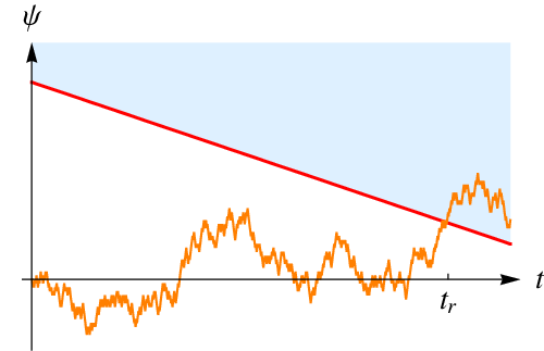
Consequently, we are interested in solving the diffusion equation (27) with an “absorbing barrier” at the corresponding value of $\psi$, i.e. the solution should satisfy the Dirichlet boundary condition

$$P|_{\psi=\psi_{r}}=0\;,$$

(28)

with

$$\psi_{r}=\phi_{r}-\dot{\phi}t=\phi_{r}-4\pi^{2}{\dot{\phi}\over H^{3}}\sigma^{2}\;.$$

(29)

Such a solution can be constructed by using a generalization of the method of images. One starts with the standard solution describing diffusion without any barriers and with initial condition localized at $\psi=0$ for $t=0$

$$P_{0}(\psi,\sigma^{2})={1\over\sqrt{2\pi\sigma^{2}}}e^{-\psi^{2}/2\sigma^{2}}\;.$$

(30)

In the case of a time independent barrier, it is well known that the Dirichlet boundary condition can be satisfied adding a negative image located specularly with respect to the barrier. In our case we have a barrier moving linearly in time. It is straightforward to show that in this case the solution becomes

$$P_{1}(\psi,\sigma^{2})={1\over\sqrt{2\pi\sigma^{2}}}\left(e^{-\psi^{2}/2\sigma^{2}}-e^{8\pi^{2}\dot{\phi}\,\phi_{r}/H^{3}}e^{-(\psi-2\phi_{r})^{2}/2\sigma^{2}}\right)\;.$$

(31)

The image is symmetric with respect to the barrier position at time $t=0$ and it is multiplied by a constant factor which depends on the barrier speed. Note that in the whole physical region, $\psi<\psi_{r}$, the contribution from the image is smaller than the $P_{0}$ term, as it should be in order for the density distribution $P_{1}$ to remain positive. Far from the barrier the contribution of the image is exponentially suppressed.

We can now use our solution for $P$ to evaluate the probability (24) of reheating at a given time $t$. By making use of the diffusion equation (27) and taking into account that $P$ vanishes on the barrier, eq. (28), we have

$$p_{r}(t)=-\frac{H^{3}}{8\pi^{2}}\left.\frac{\partial P}{\partial\phi}\right|_{\psi=\phi_{r}-\dot{\phi}t}\;.$$

(32)

Disregarding the polynomial dependence in front of the exponential we have

$$p_{r}(t)\sim e^{-2\pi^{2}\frac{(\phi_{r}-\dot{\phi}t)^{2}}{H^{3}t}}\;.$$

(33)

At late times this gives for the volume (23)

$$\langle V\rangle\simeq L^{3}\int_{0}^{\infty}dt\;\alpha(t)\,e^{3Ht-{2\pi^{2}\dot{\phi}^{2}\over H^{3}}t+O(1)}\;,$$

(34)

where the prefactor $\alpha(t)$ does not have exponential dependence on time. We see that the average reheating volume remains finite if and only if

$$\Omega\equiv{2\pi^{2}\over 3}{\dot{\phi}^{2}\over H^{4}}>1\;.$$

(35)

So far we have not talked about the initial condition we choose for the inflaton. Clearly, as the general solution of the diffusion equation is given by the convolution of $P_{1}(\psi,t)$ with the initial probability distribution, the initial condition is irrelevant for the convergence of the average reheating volume. A similar criterium for the divergence of the inflating volume was put forward in [16]. Here we focus on the more physical quantity of reheating volume and we proceed to better characterize what happens at $\Omega=1$.

Equation (35) appears as a sharp criterion for whether eternal inflation takes place or not. At the end we will argue that this is essentially correct; however to justify this conclusion we first need to address several important subtle points. Let us try to understand in more detail what happens to the probability distribution for the reheating volume $\rho(V)$ at the critical value $\Omega=1$, where the average reheating volume diverges. There are two possible options. First, it may happen that each moment $\langle V^{n}\rangle$ of the distribution has a different critical value of $\Omega$ when it starts diverging. This would happen, for instance, if $\rho(V)$ had a power law asymptotics at large values of $V$ with the power depending on $\Omega$, e.g.

$$\rho(V)\propto{1\over 1+V^{1+\Omega}}\;.$$

(36)

If this were the case, the value $\Omega=1$ associated to the divergence of $\langle V\rangle$ would not really mark any sharp transition in the physical behavior. Each moment of the distribution would single out a different transition point. Perhaps in this case a better characterization of the onset of eternal inflation would be given by the value of $\Omega$ where the probability distribution itself ceases to be normalizable ($\Omega=0$ for the model distribution (36)), if such a value exists.

The other possibility is that at $\Omega=1$ all moments of the probability distribution becomes infinite, including the “zeroth” moment, i.e. the probability distribution also ceases to be normalizable at this point. This would happen, for instance, for a family of probability distributions of the form

$$\rho(V)\propto q(V)e^{(1-\Omega)V}\;,$$

(37)

where $q(V)$ has a power-law behavior at large $V$. In this case the critical value $\Omega=1$ indeed has a very sharp physical meaning.

We will see that the actual answer is somewhat more complicated than both of these options. However, already at this point it is possible to argue that in the setup we are considering the distribution is not of the type (37) and that different moments diverge at different values of $\Omega$. Indeed, it is straightforward to see that for any given value of $\Omega$ there is a value $n_{0}$ such that all moments of the volume distribution $\langle V^{n}\rangle$ with $n>n_{0}$ diverge. Indeed, let us imagine that $\Omega$ is much larger than one, so that naively one is very far from the eternal inflation regime. Let us consider a class of inflaton trajectories that at time $t$ in one Hubble patch have a huge quantum fluctuation in the direction opposite to the classical motion, such that the inflaton ends at

$$\phi=\phi_{r}-\dot{\phi}t\;.$$

(38)

The classical trajectory would have $\phi=\dot{\phi}t$, so that at large $t$ the probability of such a fluctuation is exponentially suppressed by a factor of order $e^{-A\cdot Ht}$, with $A\sim\dot{\phi}^{2}/H^{4}\sim\Omega^{2}$. The important point is that the exponent grows only linearly with time (and not quadratically). The reason is that the variance $\sigma^{2}$ of the inflaton perturbation $\psi$ is itself a linear function of $t$. Then, with probability close to one such a trajectory will give rise to a reheated volume at least as big as $e^{3Ht}H^{-3}$, since this is the volume one would get just classically rolling down from $\phi=\phi_{r}-\dot{\phi}t$ to $\phi=\phi_{r}$. Consequently, for $n>A/3\sim\Omega^{2}$ the contribution to the moment $\langle V^{n}\rangle$ from this set of trajectories grows exponentially as a function of $t$—the large power of the exponentially growing volume over-compensates for the small probability of the required fluctuation—and these moments diverge.

At this point one is tempted to conclude that the situation is analogous to what happens with the distribution (36) and that there is no sharp transition to the eternal inflation regime. We will argue later that this conclusion is too quick, and that instead there is a sharp transition. Notice that for the rough argument about higher moments to work, it is essential to consider, as time grows, backward fluctuations that go further and further along the potential without bound. To see what this implies, it is instructive to understand the effect we just described at a more quantitative and detailed level. For this purpose we are going to study now the behavior of $\langle V^{2}\rangle$ and show that indeed it starts diverging at a critical value $\Omega>1$, i.e. when the average volume $\langle V\rangle$ is still finite.

The calculation we did for the average is deceivingly simple as the only thing we needed was the 1-point probability $P(\phi,t)$ to have a value of the field $\phi$ at time $t$, which is clearly independent of the comoving position $\vec{x}$. However the study of the full probability for the reheating volume $\rho(V)$ is not straightforward as the only expression for it is based on a functional integration over the field realizations

$$\rho(V)=\int\!{\cal D}\phi\>{\cal P}[\phi]\>\delta\big(V-\textstyle{\int}\!d^{3}x\,e^{3Ht_{r}(\vec{x})}\big)\;,$$

(39)

where ${\cal D}\phi$ is the functional measure on the set of all possible space-time realizations of the inflaton field, ${\cal P}[\phi]$ is the probability of a specific realization and $t_{r}(\vec{x})$ is the reheating time for a given realization as a function of the comoving coordinate $\vec{x}$.

Instead of trying to evaluate the expression above, to calculate $\langle V^{2}\rangle$ we will follow a procedure similar to the one used for the average. Namely, let us define the 2-point probability distribution of the inflaton field $P_{2}(\phi_{1},\phi_{2},|\vec{x}_{1}-\vec{x}_{2}|,t_{1},t_{2})$, such that

$$P_{2}\,d\phi_{1}d\phi_{2}$$

(40)

gives the joint probability of finding the inflaton field in the ranges $(\phi_{1(2)},\phi_{1(2)}+d\phi_{1(2)})$ at the two space-time points $(\vec{x}_{1},t_{1})$ and $(\vec{x}_{2},t_{2})$. For translational and rotational invariance this joint probability just depends on the distance between the two points $|\vec{x}_{1}-\vec{x}_{2}|$. Analogously to the previous section we can define a probability density $p_{2r}(t_{1},t_{2},|\vec{x}_{1}-\vec{x}_{2}|)$ for reheating to happen at the comoving point $\vec{x}_{1}$ at time $t_{1}$ and at the comoving point $\vec{x}_{2}$ at time $t_{2}$. Similarly to (24) this will be related to $P_{2}$ by

$$p_{2r}(t_{1},t_{2},|\vec{x}_{1}-\vec{x}_{2}|)=-\partial_{t_{1}}\partial_{t_{2}}\int^{\phi_{r}}_{-\infty}\!d\phi_{1}\int^{\phi_{r}}_{-\infty}\!d\phi_{2}\;P_{2}(\phi_{1},\phi_{2},|\vec{x}_{1}-\vec{x}_{2}|,t_{1},t_{2})\;.$$

(41)

Then the expectation value of $V^{2}$ can be written as

$$\langle V^{2}\rangle=\left\langle\int d^{3}x\,d^{3}y\,e^{3Ht_{r}(\vec{x})}\,e^{3Ht_{r}(\vec{y})}\right\rangle=L^{3}\int\!dt_{1}dt_{2}d^{3}x\;e^{3Ht_{1}}e^{3Ht_{2}}\;p_{2r}(t_{1},t_{2},|\vec{x}|)\;.$$

(42)

To study the convergence of this integral we need to find the 2-point probability $P_{2}$. For fixed comoving distance $|\vec{x}|$ between the two points this probability has a very different behaviour at early and late times. At early times,

$$t_{1},t_{2}\ll t_{*}\equiv-{H^{-1}}{\log H|\vec{x}|}\;,$$

(43)

the two points are within one Hubble patch and therefore they are not resolved by the smoothing procedure. As such their evolution is perfectly correlated. In particular the 2-point distribution at equal times $t_{1}=t_{2}$ is just given by the 1-point distribution (31),

$$P_{2}(\psi_{1},\psi_{2},|\vec{x}|,t,t)\simeq P_{1}(\psi_{1},t)\delta(\psi_{1}-\psi_{2})\quad\mbox{ for }\quad t\ll t_{*}(|\vec{x}|)\;.$$

(44)

In the opposite limit, when the distance is much larger than the Hubble radius, the inflaton fluctuations at the two points are completely uncorrelated. In this case, the probability distribution $P_{2}$ satisfies a diffusion equation with respect to each pair of variables $(t_{1},\phi_{1})$, $(t_{2},\phi_{2})$,

$${\partial P\over\partial\sigma_{1(2)}^{2}}={1\over 2}{\partial^{2}P\over\partial\psi_{1(2)}^{2}}\quad\mbox{ for }\quad t_{1},t_{2}\gg t_{*}\;.$$

(45)

In the equations above $\psi_{1(2)}$ and $\sigma^{2}_{1(2)}$ are related to $t_{1(2)}$ and $\phi_{1(2)}$ by the relations (25) and (26).

In the following we are going to use a “two steps” approximation in which we consider a single random walk before $t_{*}$ and two uncorrelated ones after $t_{*}$, as dipicted in figure 3 (⁶⁶ 6 The same approximation has been used in the study of structure formation in [18].).

The exact solution is more complicated as there is an intermediate period of partial correlation [18]. However it will be easy to check that our results will not depend on the exact definition of $t_{*}$, when the two regimes are matched. This strongly indicates that taking into account the period of partial correlation would not change the range of $\Omega$ when $\langle V^{2}\rangle$ converges.

In this 2-step approximation, the 2-point probability when the distance between the two points is larger than Hubble is obtained first following a single random walk until the time of “separation” $t_{*}$ and then convolving this initial condition with two independent Green’s functions for the diffusion equation with a barrier. This translates into

$$P_{2}(\psi_{1},\psi_{2},|\vec{x}|,t_{1},t_{2})=\int_{-\infty}^{\phi_{r}-\dot{\phi}t_{*}}\!\!\!\!d\psi\,G(\psi_{1},\psi,t_{1}-t_{*})G(\psi_{2},\psi,t_{2}-t_{*})P_{1}(\psi,t_{*})\;,$$

(46)

with $t_{1},t_{2}>t_{*}$. Notice that the dependence on $|\vec{x}|$ is hidden in $t_{*}$, given by equation (43). The Green’s function $G$ is straightforward to construct by making use of the solution (31). Namely, it is equal to

$$G(\psi_{1},\psi,t)=\tilde{P}_{1}(\psi_{1}-\psi,t-t_{*})$$

(47)

where “tilde” indicates that $\phi_{r}$ in eq. (31) must be replaced by

$$\phi_{r}-\psi-\dot{\phi}t_{*}$$

(48)

to take into account that the independent motion of each of the two points starts at $\psi$ at time $t_{*}$, rather than at the origin at $t=0$.

To prove that the variance diverges when the average volume is still finite, it is enough to obtain a lower bound on the integral (42). As the integrand is positive definite, we can therefore restrict the range of integration by considering only pairs of points $(\vec{x}_{1},\vec{x}_{2})$ in different Hubble patches (both at $t_{1}$ and at $t_{2}$). In other words we can impose a UV cutoff on the integration over the comoving volume in eq. (42) by requiring

$$t_{*}(|\vec{x}|)<t_{1},t_{2}\;.$$

(49)

It is anyway straightforward to check that the remaining range of integration gives a contribution that always converges whenever $\Omega>1$.

As before we can use (45) to evaluate the integrals in (41) and arrive at the following expression

$$\langle V^{2}\rangle=-{H^{6}\cdot L^{3}\over 64\pi^{4}}\int_{0}^{\infty}dt_{1}dt_{2}\int_{|\vec{x}|>H^{-1}e^{-H\tau}}\!\!\!\!\!\!\!d^{3}x\;e^{3H(t_{1}+t_{2})}\partial_{\psi_{1}}\partial_{\psi_{2}}P_{2}(\psi_{1},\psi_{2},|\vec{x}|,t_{1},t_{2})\Big|_{\psi_{1(2)}=\phi_{r}-\dot{\phi}t_{1(2)}},$$

(50)

where $\tau={\rm min}(t_{1},t_{2})$.

The partial derivatives act on each of the two Green functions of eq. (46) and give a dependence analogous to the 1-point case eq. (33). The evolution before splitting given by $P_{1}$ contains the image term and one should sum the two contributions. However, as already discussed in the previous section, we will find that the divergence of $\langle V^{2}\rangle$ is dominated by trajectories which are exponentially far from the barrier as time becomes large. This implies a posteriori that the image term is completely irrelevant.

The convolution integral in (46) can be done in saddle point approximation. The saddle point is given by

$$\psi_{\rm saddle}=t_{*}{\left(\psi_{1}+\psi_{2}\right)t_{*}-t_{2}\psi_{1}-t_{1}\psi_{2}\over t_{*}^{2}-t_{1}t_{2}}\;.$$

(51)

This gives for the exponential part of $P_{2}$

$$P_{2}(\psi_{1},\psi_{2},|\vec{x}|,t_{1},t_{2})\sim\exp{\left(-\frac{2\pi^{2}}{H^{3}}\cdot{t_{2}\psi_{1}^{2}-2t_{*}\psi_{1}\psi_{2}+t_{1}\psi_{2}^{2}\over t_{1}t_{2}-t_{*}^{2}}\right)}\;.$$

(52)

Note that this expression non-trivially depends on the spatial separation $|\vec{x}|$ through the horizon crossing time $t_{*}$, as shown in (43). To plug this result back in (50) it is convenient to use

$$t_{\pm}=t_{1}\pm t_{2}$$

(53)

as time variables and the horizon exit time $t_{*}(|\vec{x}|)$ in place of the comoving separation $\vec{x}$. With this change of variable and keeping only the leading exponential behavior at large times as in the previous section, one obtains (restricting to $t_{1}\geq t_{2}$)

$$\langle V^{2}\rangle\sim\int_{0}^{\infty}dt_{+}\,e^{3Ht_{+}}\int_{0}^{t_{+}}dt_{-}\int_{0}^{t_{+}-t_{-}\over 2}\!\!\!\!dt_{*}\,e^{-f(t_{+},t_{-},t_{*})}\;,$$

(54)

where

$$f(t_{+},t_{-},t_{*})=3Ht_{*}+3H\Omega\left(t_{+}-2t_{*}+{4t_{*}^{2}(t_{+}-2t_{*})\over t_{+}^{2}-t_{-}^{2}-4t_{*}^{2}}\right)\;.$$

(55)

The first term on the right hand side of this equation comes from the change of integration measure from $x$ to $t_{*}(|\vec{x}|)$. To check whether the integral over $t_{+}$ converges, we can minimize the function $f$ with respect to $t_{-}$ and $t_{*}$ in the range of integration. As $t_{-}$ enters into $f$ only in the denominator of the last term, it is clear that the saddle point is

$$t_{-}=0\;.$$

(56)

Then the minimization with respect to $t_{*}$ gives

$$t_{*min}={t_{+}\over 2}\left(\sqrt{2\Omega}-1\right)\;,$$

(57)

and the value of $f$ at this minimum is

$$f(t_{+},0,t_{*min})=3Ht_{+}\left(\sqrt{2\Omega}-{1\over 2}\right)\;.$$

(58)

This grows faster than $3Ht_{+}$ for

$$\Omega>{9\over 8}\;.$$

(59)

We conclude that $\langle V^{2}\rangle$ ceases to be finite when the parameter $\Omega$ drops below $9/8$, i.e. before the average volume $\langle V\rangle$ starts diverging. As a consistency check of the calculation, note that at $\Omega=9/8$ the optimal horizon exit time $t_{*min}$ indeed belongs to the integration interval in (54). For $\Omega>2$ this would no longer be true and the dominant contribution would come from $t_{*}=t_{+}/2$: $\langle V^{2}\rangle$ would be dominated by the dynamics before the two points become independent.

The above explicit calculation of $\langle V^{2}\rangle$ nicely fits into the general argument presented at the end of section 2.1. We have seen that, in saddle point approximation, the dominant contribution to $\langle V^{2}\rangle$ comes from points that reheat at the same time $t_{1}=t_{2}$. These points start evolving independently when separated by a physical distance $\sim H^{-1}$; this happens at a fraction of the eventual reheating time, which is equal to $1/2$ for the critical value $\Omega=9/8$, see (57).

Where is the most likely position along the potential at $t_{*}$, when the two points start their independent evolution? From the saddle point result (51) we see that it is a position with a huge backward fluctuation with respect to the classical trajectory

$$\psi=-\sqrt{2\over\Omega}\dot{\phi}\,t_{*min}\;.$$

(60)

For $\Omega<2$ this fluctuation corresponds to a negative value of the inflaton

$$\phi=\left(1-\sqrt{2/\Omega}\right)\cdot\dot{\phi}t_{*min}\,,$$

(61)

so that the most likely position at $t_{*min}$ is higher than the starting point at $t=0$ and it becomes higher and higher without bound for $t_{*min}\to\infty$. This agrees with the general argument above ⁷⁷ 7 Notice that as $\langle V^{2}\rangle$ is dominated by a splitting point infinitely far away from the barrier it is justified disregarding the image terms of the probability $P_{1}$ in (46)..

To summarize, all this sounds as if the volume distribution has qualitative properties similar to the model distribution (36), where the various moments start diverging at different values of $\Omega$. Thus it seems that the value $\Omega=1$, where the average volume diverges, does not really correspond to any sharp physical transition. However this conclusion is too quick. In section 3, where we study a discretized version of the same system, we will argue that at $\Omega=1$ another sharp transition occurs besides the divergence of $\langle V\rangle$: the total probability of having a finite reheating volume becomes smaller than one! This property is expected in the transition into the eternal inflation regime as it tells us that there is a finite probability of an infinite reheating volume or equivalently for inflation to last forever. Clearly this sharply defines $\Omega=1$ as the transition point to eternal inflation. Before moving to this issue, let us conclude our study of the moments of the distribution $\rho(V)$.

As we stressed, the divergence of the higher moments is qualitatively different with respect to the case of the average. The explicit calculation of $\langle V^{2}\rangle$, following the general argument made in section 2.1, shows that the divergence is related to the possibility of fluctuating uphill without bound, infinitely far from the barrier. What we are going to check is that, if we put a bound to the possibility of going infinitely uphill, all the moments diverge at the same critical value $\Omega=1$.

To impose a limit on fluctuations infinitely far from the reheating point, we can put a reflecting barrier so that the field value is constrained to satisfy

$$\phi>\phi_{up}\;,$$

(62)

where $\phi_{up}$ will be a large negative value. The value of $\psi$ at the barrier will be given by

$$\psi_{up}=\phi_{up}-\dot{\phi}t\;.$$

(63)

Here we are going to study the effect of this new barrier on the calculation of $\langle V^{2}\rangle$, while we postpone the discussion about all higher moments to Appendix A. We do not need to find the explicit form of the solution of the diffusion equation with two barriers. To keep track of the late time exponential behavior for large enough $|\phi_{up}|$, it is enough to consider that the integration range in the convolution (46) is now restricted to $(\psi_{up},\psi_{r})$ and it is not extended infinitely uphill. For $\Omega<2$ the saddle point position (61) moves backwards and thus it eventually hits the new uphill barrier. The saddle point exits the physical region and therefore, in the leading exponential approximation, the result will be dominated by a splitting point position on the uphill barrier, i.e. the point closest to the (would-be) saddle. In this approximation one obtains for the 2-point distribution

$$P_{2}(\psi_{1},\psi_{2},|\vec{x}|,t_{1},t_{2})\simeq\exp{\left[-\frac{2\pi^{2}}{H^{3}}\left({\left(\psi_{1}-\psi_{up}\right)^{2}\over t_{1}-t_{*}}+{\left(\psi_{2}-\psi_{up}\right)^{2}\over t_{2}-t_{*}}+{\psi_{up}^{2}\over t_{*}}\right)\right]}\;.$$

(64)

We are interested in the late time behaviour of this expression. The position of the uphill barrier $\phi_{up}$ becomes irrelevant in this limit as it is dominated in (63) by the time dependent term. This means that $\phi_{up}$ disappears from the calculations and therefore from the final critical value of $\Omega$ and it can be thought just as a regulating device, which can be sent to infinity. Notice however that its effect is crucial. Mathematically this comes from the fact that the large $\phi_{up}$ limit and the late time limit do not commute, because the saddle point (51) eventually exits the integration region at any finite value of $\phi_{up}$. In more physical terms this means that no matter how far the barrier is there will be a sufficient large time such that

$$H^{3}t\gtrsim\phi_{up}^{2}$$

(65)

so that the diffusion is so large to be sensitive to the presence of the extra barrier. As the transition to eternal inflation is sensitive to arbitrarily large times, the presence of the regulating barrier will be important, independently on how far we put it.

To see that the presence of the second barrier changes the value at which $\langle V^{2}\rangle$ diverges, let us plug (64) in the expression (50) for the $\langle V^{2}\rangle$. We obtain the same result as (54) with the function $f$ now taking the form

$$f(t_{+},t_{-},t_{*})=3Ht_{*}+3H\Omega\left(t_{+}-t_{*}\right)$$

(66)

We see that now the integral for $\langle V^{2}\rangle$ converges for $\Omega>1$. Note that the integral over $t_{*}$ is saturated at the upper limit, justifying a posteriori an assumption implicit in the whole derivation—that in the late time limit (meaning large $t_{1,2}$ limit) $t_{*}$ also indefinitely grows.

On the other hand it is easy to check that there is no effect of the second barrier on the calculation of $\langle V\rangle$; this is just a consequence of the fact that solutions to the diffusion equation behave continuously when one removes one of the barriers to infinity. This is checked in Appendix A, where we study the explicit solution in the presence of two barriers.

In conclusion, in the presence of an uphill regulating barrier, $\Omega=1$ is the critical point both for $\langle V\rangle$ and for $\langle V^{2}\rangle$. In Appendix A we will see that this holds also for all higher moments $\langle V^{n}\rangle$.

The bacteria branching process described above clearly captures many of the qualitative features of the actual inflaton dynamics, but it is not totally obvious that it allows to take the continuum limit that exactly reproduces the inflationary results. To explain how this happens, let us start by describing a different discrete model, which has a straightforward continuum limit reproducing inflation. This model is harder to analyze than the bacteria process, but we will explain why the two are equivalent for our purposes.

To begin with, note that in the branching process description we have two different discretizations. First we have a discrete time step; for $N\sim e^{3}$ one step of the branching process corresponds to a time interval of order $H^{-1}$. Second, the possible values of the inflaton field are discretized as well, and labeled by the bacteria positions. However, to reproduce the inflationary results we do not actually need to get rid of the time discretization. Indeed, as discussed in section 1.3, a space-time smoothing of the scalar field over the scale $\Lambda^{-1}\gtrsim H^{-1}$ is understood in all our calculations. The physical results, such as the transition point, do not depend on the details of the smoothing procedure and an explicit space-time discretization (as in the branching process approach) is as good as the smooth filter (12). Hence we only need to take the continuum limit in field space to reproduce the continuum results.

In the “two steps” approximation we have been using in studying inflation—see the discussion below eq. (45)—the inflaton dynamics is fully determined by the diffusion equation for the probability of the inflaton values at one point in spacetime, or equivalently, by the gaussian distribution (30) for the inflaton fluctuations. A straightforward way to approximate this dynamics by a branching process is to consider the following sequence of processes. For the $k$-th process of the sequence at each step every bacterium splits into $\tilde{N}$ copies. Then each bacterium hops with probabilities $p_{i}$ ($i=-k,\dots,k$) to the $2k$ adjacent sites (see Fig. 5).

As $k$ goes to infinity we require the probabilities $p_{i}$ approach the shifted gaussian distribution. In principle, all general results about branching processes described below apply to this process as well. We will refer to this process as the “gaussian model”, as opposed to the bacteria model discussed before. Clearly, the latter is much more tractable for explicit calculations.

Fortunately, for our purposes the two processes are equivalent. Indeed, let us start with a bacteria process where at every time-step each bacterium divides into $N$ copies. Equivalently, one can consider another process, where at each step a bacterium divides into $\tilde{N}=N^{k}$ copies, which then hop to the $2k$ adjacent sites with probabilities $p_{i}$ generated by iterating $k$ times the elementary process. Obviously, the late time properties of the two processes, such as the average number of dead bacteria, or whether all bacteria die or not, are the same. The two processes are in fact one and the same—only in the latter case we are observing the system less frequently, every $k$ time-steps. Also, by the central limit theorem, at large $k$ the probabilities $p_{i}$ generated in this way approach a gaussian distribution, so one gets the gaussian model.

References

- [1] J. M. Maldacena, “Non-Gaussian features of primordial fluctuations in single field inflationary models,” JHEP 0305, 013 (2003) [arXiv:astro-ph/0210603].
- [2] A. D. Linde, “Eternally Existing Selfreproducing Chaotic Inflationary Universe,” Phys. Lett. B 175, 395 (1986).
- [3] A. S. Goncharov, A. D. Linde and V. F. Mukhanov, “The Global Structure Of The Inflationary Universe,” Int. J. Mod. Phys. A 2 (1987) 561.
- [4] A. H. Guth, “The Inflationary Universe: A Possible Solution To The Horizon And Flatness Problems,” Phys. Rev. D 23 (1981) 347.
- [5] A. D. Linde, “Nonsingular Regenerating Inflationary Universe,” Cambridge University preprint Print-82-0554 (1982).
- [6] P. J. Steinhardt, “Natural Inflation,” in The Very Early Universe , ed. G.W. Gibbons, S.W. Hawking and S. Siklos, Cambridge University Press, (1983).
- [7] A. Vilenkin, “The Birth Of Inflationary Universes,” Phys. Rev. D 27 (1983) 2848.
- [8] A. H. Guth, “Eternal inflation and its implications,” J. Phys. A 40 (2007) 6811 [arXiv:hep-th/0702178].
- [9] A. Linde, “Prospects of inflation,” Phys. Scripta T117 (2005) 40 [arXiv:hep-th/0402051].
- [10] D. Seery, J. E. Lidsey and M. S. Sloth, “The inflationary trispectrum,” JCAP 0701, 027 (2007) [arXiv:astro-ph/0610210].
- [11] A. D. Linde, “Eternal Chaotic Inflation,” Mod. Phys. Lett. A 1, 81 (1986).
- [12] A. Vilenkin and L. H. Ford, “Gravitational Effects Upon Cosmological Phase Transitions,” Phys. Rev. D 26, 1231 (1982).
- [13] A. D. Linde, “Scalar Field Fluctuations In Expanding Universe And The New Inflationary Universe Scenario,” Phys. Lett. B 116, 335 (1982).
- [14] A. A. Starobinsky, “Dynamics Of Phase Transition In The New Inflationary Universe Scenario And Generation Of Perturbations,” Phys. Lett. B 117 (1982) 175.
- [15] A.A. Starobinsky, in: Fundamental Interactions (MGPI Press, Moscow, 1984, p. 55; A.A. Starobinsky, in: Current Topics in Field Theory, Quantum Gravity and Strings, Lecture Notes in Physics, eds. H.J. de Vega and N. Sanchez (Springer, Heidelberg 1986), 206 p. 107.
- [16] S. Winitzki, “The eternal fractal in the universe,” Phys. Rev. D 65, 083506 (2002) [arXiv:gr-qc/0111048].
- [17] D. Polarski and A. A. Starobinsky, “Semiclassicality and decoherence of cosmological perturbations,” Class. Quant. Grav. 13, 377 (1996) [arXiv:gr-qc/9504030].
- [18] E. Scannapieco and R. Barkana, “An Analytical Approach to Inhomogeneous Structure Formation,” arXiv:astro-ph/0205276.
- [19] K. B. Athereya, P. E. Ney, “Branching Processes,” Berlin: Springer ( 1972); T. E. Harris “The Theory Branching Processes,” Berlin: Springer ( 1963).
- [20] S. Winitzki, “On time-reparametrization invariance in eternal inflation,” Phys. Rev. D 71, 123507 (2005) [arXiv:gr-qc/0504084].
- [21] J. Garriga and V. F. Mukhanov, “Perturbations in k-inflation,” Phys. Lett. B 458, 219 (1999) [arXiv:hep-th/9904176].
- [22] M. Alishahiha, E. Silverstein and D. Tong, “DBI in the sky,” Phys. Rev. D 70, 123505 (2004) [arXiv:hep-th/0404084].
- [23] N. Arkani-Hamed, P. Creminelli, S. Mukohyama and M. Zaldarriaga, “Ghost inflation,” JCAP 0404, 001 (2004) [arXiv:hep-th/0312100].
- [24] L. Senatore, “Tilted ghost inflation,” Phys. Rev. D 71, 043512 (2005) [arXiv:astro-ph/0406187].
- [25] P. Creminelli, M. A. Luty, A. Nicolis and L. Senatore, “Starting the universe: Stable violation of the null energy condition and non-standard cosmologies,” JHEP 0612, 080 (2006) [arXiv:hep-th/0606090].
- [26] C. Cheung, P. Creminelli, A. L. Fitzpatrick, J. Kaplan and L. Senatore, “The Effective Field Theory of Inflation,” arXiv:0709.0293 [hep-th].
- [27] D. Seery and J. E. Lidsey, “Primordial non-gaussianities in single field inflation,” JCAP 0506, 003 (2005) [arXiv:astro-ph/0503692].
- [28] X. Chen, M. x. Huang, S. Kachru and G. Shiu, “Observational signatures and non-Gaussianities of general single field inflation,” JCAP 0701, 002 (2007) [arXiv:hep-th/0605045].
- [29] M. x. Huang and G. Shiu, “The inflationary trispectrum for models with large non-Gaussianities,” Phys. Rev. D 74, 121301 (2006) [arXiv:hep-th/0610235].
- [30] N. Arkani-Hamed, S. Dubovsky, A. Nicolis, E. Trincherini and G. Villadoro, “A Measure of de Sitter Entropy and Eternal Inflation,” JHEP 0705, 055 (2007) [arXiv:0704.1814 [hep-th]].
- [31] X. Chen, S. Sarangi, S. H. Henry Tye and J. Xu, “Is brane inflation eternal?,” JCAP 0611 (2006) 015 [arXiv:hep-th/0608082].
- [32] L. Leblond and S. Shandera, “Simple Bounds from the Perturbative Regime of Inflation,” arXiv:0802.2290 [hep-th].
- [33] N. Arkani-Hamed, S. Dubovsky, L. Senatore and G. Villadoro, “(No) Eternal Inflation and Precision Higgs Physics,” arXiv:0801.2399 [hep-ph].
- [34] A. Strominger, “The dS/CFT correspondence,” JHEP 0110, 034 (2001) [arXiv:hep-th/0106113].
- [35] A. H. Guth and E. J. Weinberg, “Could The Universe Have Recovered From A Slow First Order Phase Transition?,” Nucl. Phys. B 212, 321 (1983).
- [36] A. Vilenkin, “Topological inflation,” Phys. Rev. Lett. 72, 3137 (1994) [arXiv:hep-th/9402085].
- [37] A. D. Linde, “Monopoles as big as a universe,” Phys. Lett. B 327 (1994) 208 [arXiv:astro-ph/9402031].