Volume modulus inflation and a low scale of SUSY breaking
M. Badziak and M. Olechowski
Institute of Theoretical Physics, University of Warsaw
ul. Hoża 69, PL–00–681 Warsaw, Poland
Abstract
The relation between the Hubble constant and the scale of supersymmetry breaking is investigated in models of inflation dominated by a string modulus. Usually in this kind of models the gravitino mass is of the same order of magnitude as the Hubble constant which is not desirable from the phenomenological point of view. It is shown that slow-roll saddle point inflation may be compatible with a low scale of supersymmetry breaking only if some corrections to the lowest order Kähler potential are taken into account. However, choosing an appropriate Kähler potential is not enough. There are also conditions for the superpotential, and e.g. the popular racetrack superpotential turns out to be not suitable. A model is proposed in which slow-roll inflation and a light gravitino are compatible. It is based on a superpotential with a triple gaugino condensation and the Kähler potential with the leading string corrections. The problem of fine tuning and experimental constraints are discussed for that model.
1 Introduction
The existence of an inflationary stage in the very early Universe is a paradigm of the contemporary cosmology. Inflation solves many problems of the standard cosmology, such as flatness and isotropy of the observed Universe. It provides also the best known mechanism to generate the primordial density fluctuations. This feature of inflation makes it testable by means of the CMB spectrum which is measured very precisely by WMAP and will be measured even better by the forthcoming Planck satellite.
Inflation is usually implemented via dynamics of a scalar field - the inflaton. The scalar sector of the Standard Model contains only the Higgs field and its potential cannot accommodate inflation. Thus, inflation can be realized only in some (more fundamental) generalization of the Standard Model. The most promising candidates for “the theory of everything” are 10-dimensional string theories. To make contact with our low-energy 4-dimensional world, six of these dimensions have to be compactified. The main obstacle which for many years prevented from doing phenomenology within string theories was lack of a potential for the moduli fields parametrizing 6-dimensional internal manifolds. The breakthrough in the moduli stabilization was made within the framework of type IIB string theory, the dilaton and the complex structure moduli (CSM) were stabilized by turning on some non-trivial fluxes [1]. A mechanism to stabilize also the Kähler moduli, including the volume modulus, was proposed in the famous KKLT model [2]. It uses nonperturbative effects, such as the gaugino condensation, which give rise to terms in the superpotential11 1 In the KKLT model it is assumed that the dilaton and the CSM are stabilized at high energies and nonperturbative effects do not destabilize them. In [3] a detailed analysis of the validity of this assumption was done. It was found that in the simplest model without CSM moduli stabilization cannot be achieved. depending exponentially on the volume modulus. As a result, the volume modulus is stabilized in a supersymmetric (SUSY) anti de Sitter (AdS) minimum which, after inclusion of anti-branes, is uplifted to a de Sitter (dS) space. The main drawback of this model is the explicit breaking of SUSY by anti-branes. However, this part of the KKLT model has been improved and the moduli have been stabilized in dS vacua with SUSY broken spontaneously by F-terms [4]-[11] or D-terms [12]-[14].
Development of dS string vacua opened the possibility of constructing inflationary models within string theories. There are two types of scenarios: One is brane inflation, where the interbrane distance plays the role of the inflaton [15]-[16]. The other one is moduli inflation, where the inflaton is one of the moduli fields. In this paper, we concentrate on the latter scenario. In the KKLT model with only one exponential term in the superpotential, the potential is too steep for slow-roll inflation. However, adding second exponential term to the superpotential makes inflation possible. This was done in [17] where a model called the racetrack inflation was proposed. It is a model with one Kähler modulus, the volume modulus. Its imaginary part plays the role of the inflaton. Similarly as in the KKLT model, a dS vacuum is obtained by non-supersymmetric uplifting. Racetrack inflation models with supersymmetric uplifting have been also constructed. A model with string theory -corrections as a source of uplifting and with SUSY broken in a dS vacuum by nonvanishing F-terms was presented in [18]. D-terms were used to uplift the potential in racetrack inflation in [19]. The racetrack inflation model was generalized to the case of two Kähler moduli in [20]. Other models of moduli inflation were proposed in [21]-[22].
It was pointed out in [23] that in inflationary models based on the KKLT moduli stabilization, the gravitino mass is typically of the order of the Hubble scale during inflation which should be many orders of magnitude larger than the electroweak scale. Models with such heavy gravitino (typically much above the TeV scale) are disfavored from the phenomenological point of view. A possible solution to this problem was proposed in [23] where it was observed that in models with a SUSY Minkowski vacuum the gravitino mass is not directly related to the scale of inflation. Such SUSY Minkowski vacua exist in KKLT type models with the racetrack superpotentials (an additional tuning of parameters is necessary). We will call it the Kallosh-Linde (KL) model.
In [24] an inflationary model based on the KL model was constructed. However, in this model the moduli are stabilized in a non-SUSY Minkowski minimum, which was obtained by uplifting an AdS minimum (existing in addition to the SUSY Minkowski one). Therefore, in this model the gravitino mass is also much larger than the TeV scale.
The main goal of this paper is to construct an inflationary model, within the framework of type IIB string theory, with the gravitino mass much smaller than the Hubble constant during inflation. We restrict ourselves to models with only one Kähler modulus (the volume modulus) and assume that the dilaton and the CSM are stabilized by fluxes at some higher scales. The results of our investigation should be valid also for multi-field models with inflation dominated by the volume modulus. We focus on inflation that occurs in the vicinity of the saddle point with the inflaton rolling down towards the SUSY Minkowski minimum at which the gravitino mass vanishes (or near-Minkowski minimum at which the gravitino mass is very small). In order to find flat enough saddle points, which are necessary for slow-roll inflation, we perform a general study of non-SUSY stationary points with arbitrary Kähler potential and superpotential. We derive a necessary condition for slow-roll inflation. Then, we focus on the string inspired Kähler potentials and show that, for a tree-level Kähler potential and an arbitrary superpotential, inflation that finishes in the SUSY Minkowski minimum cannot be realized. We find that the perturbative corrections to the Kähler potential can improve somewhat the situation but even with such corrections, inflation still cannot be implemented in the KL model.
We propose a model in which inflation with the Hubble constant much bigger than the gravitino mass can be realized. It is based on a superpotential with three exponential terms that may originate from the gaugino condensation in a hidden sector. We use also the Kähler potential with -corrections and string loop corrections. In this setup successful slow-roll inflation can be obtained with the spectral index consistent with the observations. The inflaton, which is mainly the imaginary part of the volume modulus, rolls down towards the SUSY near-Minkowski minimum, where inflation ends. Therefore, in this model the gravitino mass can be made very small.
The paper is organized as follows. In section 2 we analyze non-SUSY stationary points and formulate conditions necessary for slow-roll inflation. In section 3 we show how the string inspired corrections to the Kähler potential may help in fulfilling such conditions. The KL model is analyzed in section 4. We show that slow-roll inflation can not be realized in racetrack models with SUSY Minkowski minimum even with the corrected Kähler potential. In section 5 we propose a triple gaugino condensation model. It can accommodate slow-roll inflation with the Hubble constant much bigger than the gravitino mass. We study predictions of this model and show that they are compatible with current observational status. Finally, we conclude in section 6.
2 Non-supersymmetric stationary points
The scalar potential in supergravity can be expressed in terms of the superpotential and the Kähler potential in the following way22 2 We use Planck units where . :
| (1) |
Supersymmetric stationary points of this potential satisfy the condition:
| (2) |
Using (2) and (1), we immediately see that the value of the potential at a SUSY stationary point is always non-positive and vanishes only when
| (3) |
Models with SUSY Minkowski vacua within type IIB string theory were studied in [25]. In [26] it was shown that any Minkowski vacuum, satisfying conditions (3), is stable. Of course, the gravitino mass vanishes in a SUSY Minkowski vacuum.
We are interested in inflation ending in a SUSY (near) Minkowski vacuum. Inflation may end in a Minkowski vacuum if it starts from the vicinity of a (nearby) saddle point with positive energy. In [27] the necessary conditions for the stability of non-SUSY Minkowski vacua were found. In what follows, we generalize those results for any non-SUSY stationary points.
For this analysis, it is convenient to work with function defined by:
| (4) |
In terms of , the scalar potential can be written as33 3 We use the standard notation , . :
| (5) |
Following [27], we use the tools of Kähler geometry with the metric given by the second derivative of the Kähler potential . A covariant derivative of a scalar is equal to an ordinary derivative, therefore we can write the stationarity conditions using covariant derivatives (which is more convenient):
| (6) |
The second covariant derivatives of the potential are given by
| (7) |
where is the connection for the Kähler manifold defined by the metric . We are interested in the second derivatives at stationary points, where the first derivatives vanish. At such points, the term in (7) proportional to the connection vanishes, and the ordinary second derivatives are equal to the covariant second derivatives. Therefore, the matrix of the second derivatives of the potential at a stationary point reads:
| (8) |
where the second covariant derivatives, and , are given by the following expressions:
| (9) | |||||
| (10) |
, and all quantities should be understood as evaluated at a stationary point. We introduced a quantity which is related in a simple way to the value of the potential:
| (11) |
For , which corresponds to the Minkowski condition, in each of the eqs. (9) and (10) the first term simplifies while the second one vanishes. In case of dS stationary points, which are of main interest in this paper, we have .
Expressions (9) and (10) were derived in full generality but to use them in practice one has to impose some restrictions. For the purpose of this work, it is enough to restrict to the one-field case. For non-canonically normalized fields the physical mass matrix is given by
| (12) |
with the entries
| (13) |
which can be written in the following form:
| (14) | |||||
| (15) |
where , , , etc…. The curvature scalar of the Kähler manifold, , is given by:
| (16) |
Notice that all quantities in contain derivatives of with respect to both holomorphic and anti-holomorphic variables. So, does not depend on the superpotential (which is holomorphic) and is fully determined by the Kähler potential . In the case of stationary points satisfying the Minkowski condition, i.e. , the diagonal entry of the mass matrix (12) depends on the superpotential only via the overall factor because the Minkowski condition fixes the value of . On the other hand, looking for a saddle point appropriate for inflation, we do not insist on any particular value of the potential at such point. It only has to be positive. Therefore, we do not fix the value of , and from (14) one can see that does depend on both the Kähler potential and the superpotential.
In the one-field case the mass eigenvalues can be computed analytically:
| (17) |
When constructing a model of inflation, one usually deals with real fields rather than with complex ones. It is convenient to introduce a new object, the so-called -matrix, which is defined for real fields and is very useful when looking for models appropriate for inflation. The entries of the -matrix are given by the second covariant derivatives with respect to real fields in the following way:
| (18) |
where and the lower case indices correspond to imaginary or real parts of complex fields (represented by capital letter indices). The smallest eigenvalue of the -matrix is a multi-field generalization of the slow-roll parameter . Inflation can take place in the vicinity of a saddle point for which the parameter is very small and negative while all other eigenvalues of the -matrix are positive. In other words, this saddle point should be very flat in the unstable direction. At the stationary points the entries of the -matrix are proportional to the corresponding entries of the mass-matrix, and this flatness condition, in the one-field case, can be formulated as:
| (19) |
where is the value of the potential at the stationary point. In principle, one could use the above condition together with (14) and (15) to look for models suitable for inflation. However, depends on and in a very complicated way (eq. (15)), so it may turn out to be a highly non-trivial task. On the other hand, a necessary condition for a successful model of inflation says that the trace of the -matrix is positive44 4 To be strict, slow-roll inflation could be possible also for slightly negative trace of the -matrix. It would require one very small negative eigenvalue and the other one with even smaller absolute value. However, this would require more fine tuning of parameters. It is also very unlikely from the observational point of view because it would provide very significant production of isocurvature fluctuations, which has not been observed. For the recent study on the isocurvature perturbations see e.g. [28]. . It is relatively simple:
| (20) |
and, using eq. (14), can be rewritten as a condition for the Kähler curvature:
| (21) |
This condition involves both the Kähler potential and the superpotential. However, a superpotential-independent upper bound on the value of the Kähler curvature can be found for all dS stationary points (which are most interesting for inflation). It follows from (11) and (21) that the parameter may be small only for such stationary points for which
| (22) |
This condition is weaker than (21) but it is still an important one because it can be used to eliminate some models even without specifying the superpotential. It should be stressed that (22) is necessary but not sufficient to satisfy the condition (20). Notice also that the right-hand side of (21) is always positive, so (20) is satisfied when is negative or zero.
3 String inspired Kähler potentials
We concentrate now on the class of models motivated by string theories for which the Kähler potential is given by:
| (23) |
where is a positive integer. For the above Kähler potential the curvature scalar is constant and has a very simple form:
| (24) |
Using (14) and (11) we can formulate the following condition necessary for the existence of a flat saddle point (20):55 5 A similar result, in a different context, was obtained in [29].
| (25) |
Inflation has to start from a saddle point satisfying the above condition with a positive energy. It is clear that no such saddle points exist in models with . Whether they exist or not for , depends on details of a specific model.
For the Kähler potential (23) we find the following expression for the trace of the -matrix:
| (26) |
where Re and Im. The r.h.s. of this equation is negative for any and . It is a significant result which tells us that for any superpotential and the standard Kähler potential, slow-roll inflation dominated by one modulus and starting close to a saddle point of the potential is not possible in a broad class of models inspired by string theories.
Equation (26) simplifies in type IIB string theory (on which we focus in this paper) for which the Kähler potential for the volume modulus is given by:
| (27) |
For this setup the trace of the -matrix takes a constant negative value:
| (28) |
where Re and Im.
The condition (28) forbids saddle point inflation in supergravity theories with the Kähler potential (27). So, how is it possible that the original racetrack model [17] successfully implements inflation, even though it starts from the vicinity of a non-SUSY saddle point? To answer this question, we recall that a key ingredient of the racetrack model is the uplifting term in the potential
| (29) |
which explicitly breaks supersymmetry. The numerical value of is fine tuned in order to uplift the AdS minimum to the Minkowski one. It turns out that this term plays also a very important role from the inflationary point of view. The reason is that the uplifting gives an additional contribution to the second derivative of the potential with respect to increasing by
| (30) |
where ellipsis denotes corrections due to different position of the saddle point and the value of the potential after uplifting. Other entries of the -matrix are also changed. Slow-roll inflation is possible when is big enough at the uplifted saddle point. We have checked that for the parameters used in [17], the value of is about 4, which is substantially bigger than the limiting value . Parameter has to be large enough to increase appropriately the trace of the -matrix. So, the SUSY AdS minimum before uplifting has to be rather deep to ensure that after uplifting is big enough. As we mentioned before, a deep AdS minimum is the source of a large gravitino mass in the uplifted Minkowski minimum.
There are also racetrack inflation models with uplifting which breaks SUSY spontaneously by F-terms [18] or D-terms [19]. Such upliftings contribute to the -matrix in a more complicated way but in every case they make the trace of the -matrix positive. The main disadvantage of this class of models is a large gravitino mass. In the following sections we discuss mechanisms which can change the condition (28) without increasing a small (or even vanishing) gravitino mass.
3.1 Corrections to Kähler potential
In this subsection we identify corrections to the Kähler potential which may change the sign of the -matrix trace. A necessary condition for the positivity of that trace is
| (31) |
while a sufficient one is
| (32) |
In a type IIB model with the leading order of the Kähler potential for the volume modulus (27), the Kähler curvature equals . Therefore, the necessary condition (31) in such a model is only marginally violated, so even relatively small corrections to can make this condition satisfied. On the other hand, is far away from the sufficient condition (32).
In general, it is not hard to satisfy condition (32). For example, in the case of the simplest Kähler potential , which provides the canonical kinetic term for the field , vanishes. Unfortunately, this is not the case for the moduli fields. We check now whether corrections to the leading order Kähler potential (27) can give a negative contribution to . We consider the corrections of the following form:
| (33) |
The scalar curvature for the corrected Kähler metric reads:
| (34) |
As one can see, for and , correction (33) gives a negative contribution to . The string theoretical predictions for the corrections to the Kähler potential presented in [30] are given by:
| (35) |
where is the coefficient of the -correction and is the coefficient of the string loop correction. The leading -corrections were computed in [31] and the coefficient was found to be of the following form:
| (36) |
where is the Euler number of the compactification manifold and is the expectation value of the dilaton (which we assume to be stabilized by fluxes). The form of the leading string loop correction was found in [32] by a dimensional analysis. Further studies of the string loop corrections were done e.g. in [33]-[35] but quite little is known about the coefficient .
For those specific corrections (35), the scalar curvature reads:
| (37) |
where ellipsis stands for the higher order terms. The numerical coefficient in front of the -correction is comparable with the leading order contribution, , while the numerical coefficient in front of the string loop correction is four times bigger. Therefore, there is a chance to find saddle points with positive trace of the -matrix in the region where the corrections to the Kähler potential are small enough to trust the perturbative expansion, especially with the help of the string loop corrections.
Corrections to the leading order Kähler potential have already been used to implement inflation in type IIB string theory. In [18] a racetrack inflation model was presented in which the -corrections were used to uplift a SUSY AdS minimum to a dS space (and to break supersymmetry). In the next sections we investigate models in which the corrections to the Kähler potential are used to implement inflation, but in a different way than in [18]. We start with a SUSY Minkowski (or near-Minkowski) minimum and then add the Kähler corrections to modify the structure of the -matrix in order to satisfy the slow-roll conditions. The Kähler corrections do not affect the position of the SUSY Minkowski minimum (see (3)) so the gravitino remains massless (or at least very light).
4 Problems with inflation in Kallosh-Linde model
It was pointed out in [23] that in the KKLT-type models, there is the following relation between the scale of inflation and the gravitino mass:
| (38) |
A typical scale of inflation is much above the TeV scale, so the above relation makes a low-energy supersymmetry breaking problematic. This problem is caused by uplifting a AdS minimum to a Minkowski (or dS) space. In models with a SUSY Minkowski minimum no uplifting is needed, so this problem is evaded. The simplest model of this type is the KL model.
In this section we examine the possibility of inflation in the KL model. The superpotential in this model reads:
| (39) |
The exponential terms come from gaugino condensation in the hidden sector. The parameters and are determined by the rank of the hidden sector gauge group . Without loosing generality, we choose . The parameter is the contribution from fluxes. Conditions (3) can be solved exactly and imply a SUSY Minkowski minimum at the following value of :
| (40) |
Notice that at this minimum. The existence of a SUSY Minkowski minimum imposes the following constraint on the superpotential parameters:
| (41) |
which we will use to eliminate from all formulae in this section. The scalar potential can be written in the form:
| (42) | |||||
where and . The SUSY Minkowski minimum is located at , . The explicite dependence on the parameters and factorizes and appears only in the combination . However, there is a hidden dependence on these parameters in because depends on the ratio .
For the potential (42) one could imagine two scenarios of inflation starting at a saddle point and ending in the SUSY Minkowski minimum: one dominated by field and another dominated by . However, there are obstacles which do not allow for any of these scenarios to be realized in the KL model. First of all, as we have shown in the previous section, for any superpotential, inflation is impossible when the Kähler potential has the standard form given in eq. (27). But even for a more general Kähler potential no slow-roll inflation can be realized with the racetrack superpotential (39). It is instructive to discuss in some detail the KL model with the uncorrected Kähler potential. Then, it will be easier to understand why for the corrected Kähler potential inflation is still not possible.
4.1 as candidate for inflaton
We begin with the case for which is a candidate for the inflaton. It is easy to see that for the potential (42) has vanishing derivatives: , . So, at each for which , there is a stationary point with a diagonal matrix of the second derivatives of the potential. Some of such points may be saddle points with instability in the direction. In order to study such stationary points we compute the first derivative of (42) with set to zero66 6 We choose but one should remember that the potential (42) is periodic in with the period equal to the smallest common multiple of integers and introduced after eq. (39). :
| (43) |

The above function has three zeros which correspond to three extrema of the potential (see fig. 1). The first one is the SUSY Minkowski minimum () corresponding to the first zero of the function in the second square bracket in (43). The second one is a maximum (saddle point from the two-dimensional point of view) corresponding to the only zero of the function in the first square bracket. The third one is an AdS minimum which corresponds to the second zero of the second square bracket.
In principle, there could be a chance that inflation starts at the vicinity of the saddle point from which the inflaton slowly rolls down towards the SUSY Minkowski minimum. Therefore, we study this saddle point in more detail. Its position is given by the solution of the following equation:
| (44) |
This equation cannot be solved exactly. However, it can be solved in the limit . The approximate solution is given by:
| (45) |
For it satisfies the condition , while in the limit , we obtain . It can be shown that the exact value of is smaller than its approximate value (45).
In order to check whether slow-roll inflation is possible, we compute the parameter at the saddle point (44). Since vanishes at , -matrix is diagonal and parameter is found to be:
| (46) |
One could hope to get by tuning the second bracket in the above equation to a very small value. This would require:
| (47) |
We will show that the above approximate equality can not be fulfilled. Let us start with the limit in which eq. (44) can be solved for arbitrary value of giving:
| (48) |
This is a monotonically growing function of with the upper limit . For the minimal possible value , the above equation yields . Therefore, for , the l.h.s. of (47) equals and is smaller than the r.h.s. which equals . Observing that the r.h.s. of (47) grows faster with than the l.h.s. of (47), we conclude that, in the limit , condition (47) cannot be satisfied for any value of . It is easy to see that this conclusion remains true also for . For fixed , the r.h.s. of (47) increases with growing while , and hence the l.h.s. of (47) decreases. We have shown that the square bracket in (46) can not be very small.
The range of possible values of the parameter may be, in some approximation, found from eq. (46). In the limit , we get:
| (49) |
The smallest possible value of is obtained for and . Therefore, is never small enough and slow-roll inflation is not possible.
This result can be interpreted as a manifestation of the well-known -problem in supergravity, which states that a generic value of is of order one. This problem can be evaded for fields which do not appear in the Kähler potential. This is the case for the field . We examine the possibility that is an inflaton in the next subsection.
4.2 as candidate for inflaton


The position of the SUSY Minkowski minimum is at . Therefore, a saddle point with instability in the direction has to be situated at . The potential (42) depends on through sines of , and , which have the first maximum in the direction at , and , respectively. In the limit , the structure of the maxima in the direction is dominated by the term (the last term in (42)). Furthermore, the coefficients multiplying and have opposite signs. All this suggests that the first maximum in the direction is around . We checked numerically that for large the first maximum in the direction is indeed around . For smaller the first maximum in the direction appears at least for . To be a saddle point, such a maximum in the direction must be a minimum in the direction. We have found numerically that the minima in the direction, having positive energy, exist only for relatively small values of (see fig. 2). To understand this fact we compute the first derivative of the potential (42) for :
| (50) | |||||
The potential has, for fixed , a minimum in the direction at if vanishes at and is positive in some interval . There is no such a minimum if is negative for every , where is the value of at the AdS minimum. We discuss now in more detail the sign of for non-zero values of . The third term in (50) is always negative for . The second term in (50) is positive for small but asymptotically for large it is negative too. Expanding the second term in (50) to the second order in , we find that it changes sign for being the solution of the following equation:
| (51) |
which, in the limit , is given by:
| (52) |
Therefore, the -dependent part of , given by the last two terms in (50), could be positive only for . However, it occurs that the -dependent part of is always negative. In order to show this, we expand in :
| (53) | |||||
We are interested in the coefficient of the term. The negative terms in the square bracket in the above equation are of order , while the positive ones are of order (we recall that the -dependence is implicit via the relation ). Therefore, for a given , there always exists such that the -dependent part of is negative. Furthermore, the second term of the -expansion (53), for , is a monotonically decreasing function of :
| (54) |
So, if the second term in (53) is negative for the smallest possible value of , then it is negative for any . Thus, we concentrate now on the case . It is convenient to introduce a dimensionless parameter :
| (55) |
The coefficient of the term in (53), up to normalization, can be rewritten in the following way:
| (56) | |||||
This expression looks quite complicated but after imposing , it is the function of two variables and . >From fig. 3 one can see that the second term in (53) is always negative. This is the reason why for a certain value of the minimum in the direction disappears. The potential (42) has no saddle points which are maxima in the direction.
4.3 Corrections to Kähler potential in KL model
We have shown that the corrections to Kähler potential can help in building models of inflation. However, as we will show in this subsection, the corrections to Kähler potential are still not sufficient to implement inflation in the KL model. For simplicity we use only the -correction (the string loop corrections modify the potential in a similar way) which we denote by :
| (57) |
The resulting leading correction to the scalar potential reads:
| (58) |
As in the case without corrections, we are most interested in the term of the expansion77 7 The explicite expressions for the potential and its derivative are given in the appendix. of :
| (59) | |||||
It is a complicated expression but one can figure out some interesting features. For , the leading term in the limit (the first term in (59)) factorizes in the same way as in the uncorrected case (the first term in (53)). Therefore, the correction affects the leading term in only by a small change of an overall coefficient ( in the perturbative regime). The position of the maximum in the direction of that leading term remains unchanged. Obviously, the corrections to the non-leading terms in (53) may change this position a little bit, but in all the terms the corrections change the coefficients only by small fractions. Figure 4 shows that the position of the barrier is almost unchanged by the corrections. One can see also that the corrections make the barrier slightly higher. This decreases the parameter but only by a small amount. Therefore, we expect the parameter to be only marginally changed by the corrections. We confirmed these expectations by numerical analysis. We conclude that inflation from the saddle point in the direction is not possible in the KL model.


The -dependent part of is less complicated. Similarly to the uncorrected case, it can be shown that it is always negative. We proceed in the same way as before. For , the term proportional to in (59) is still a monotonically decreasing function of :
| (60) |
So, again it is enough to concentrate on the case with . The term proportional to in the expansion of is given by (A.3) in the appendix. The plot of this function is presented on fig. 5. One can see that even relatively large corrections do not significantly alter the results as compared to the uncorrected case. The -dependent part of is still negative. The minimum in the direction disappears for values of similar to those in the uncorrected case, as seen in fig. 4.
In this section we have shown that it is not possible to implement inflation in the KL model with or without corrections to the Kähler potential. We conclude that the realization of inflation requires not only the corrections to the Kähler potential but also some change of the form of the superpotential.
5 Triple gaugino condensation model
In this section, we show that a successful inflation in the vicinity of a SUSY Minkowski minimum can be achieved by changing the superpotential. We consider models with the superpotential containing three gaugino condensation terms:
| (61) |
We allow and to be complex (the reasons for such choice will be explained later) but, for simplicity, assume that and are real. The hidden sector gauge group is and the additional parameter in the exponential, as compared to racetrack superpotential, is . We take the Kähler potential with the leading corrections:
| (62) |
In this model the conditions (3) for the existence of a SUSY Minkowski minimum cannot be solved analytically and the solution is not unique. A new feature is the possibility of having a SUSY Minkowski minimum for a non-zero value of (this requires a non-zero imaginary part of ). Moreover, near this SUSY Minkowski minimum there exists a dS saddle point at which inflation could start. However, one can check that it is impossible to have a small -parameter if all three parameters , and are real. We performed numerical analysis of the -matrix for many different sets of the parameters: , , , , , , and , adjusting parameter to keep at the Minkowski minimum. We observed that the behaviour of the -matrix is similar if we change any of the parameters , , , , or . For concreteness, let us concentrate on changing parameter keeping other (except ) fixed. For a certain value of , the SUSY Minkowski minimum is situated at (as in the KL model) and the saddle point is unstable in the direction having very large, negative . Changing , we can move the SUSY Minkowski minimum to a non-zero value of , but a nearby saddle point has very large negative . Changing further, one can obtain very small negative . Unfortunately, the off-diagonal entry is very large, so the parameter remains also very large. For a small range of both diagonal entries of the -matrix are positive but the trace is always smaller than the off-diagonal entry. This implies again a large, negative -parameter. Changing one can also obtain very small, negative but still large off-diagonal entry prevents from the slow-roll regime. The parameters and , which parametrize the corrections to the Kähler potential, change the -matrix in a different way. All the entries of the -matrix grow with increasing or . The trace of the -matrix also grows but still it is smaller than the off-diagonal entry. We conclude that the main obstacle in obtaining a flat saddle point are large off-diagonal entries of the -matrix.
The situation changes when one allows for a small imaginary parts of , or . We choose to be complex but similar results can be obtained when choosing or to be complex88 8 Nonzero imaginary parts of , and can originate from loop threshold corrections to the corresponding gauge kinetic functions (see e.g. [36]-[37]). Such corrections usually depend logarithmically on various moduli fields and can modify gaugino condensation terms by moduli-dependent polynomial prefactors. In our model most of the moduli are assumed to be stabilized at higher scales. If some of them has complex vevs, the parameters , , can have imaginary parts. Moreover, relative phases of , and can be changed by redefining the axion . . Changing the value of , one can obtain a very small off-diagonal entry of the -matrix. Furthermore, with one more parameter (, or ) fine-tuned, a slow-roll inflation is possible. For the numerical example we choose the following set of parameters:
| (63) |
For this set of parameters the condition at the SUSY near-Minkowski minimum is obtained by tuning and in the following way:
| (64) |
The exact SUSY Minkowski minimum can be obtained only by exact tuning . However, in our world SUSY is broken and the gravitino mass does not vanish. Therefore, tuning of does not have to be very precise.
In this example we use both and string loop corrections but an inflationary saddle point can be found using or string loop correction alone. Therefore, our effective model is also valid for Calabi-Yau compactifications for which one of these corrections is suppressed.
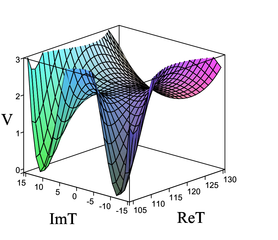
The structure of the inflationary potential is shown at fig. 6. There are two minima and the saddle point where inflation can take place. One of these minima is of AdS-type and is situated at the following field values:
| (65) |
We are more interested in the SUSY Minkowski minimum which occurs at:
| (66) |
The inflationary saddle point is situated at:
| (67) |
In order to trust the perturbative expansion of the Kähler potential, the ratios and has to be small. For the Minkowski minimum (66) these turn out to be, respectively, around and , while for the saddle point (67) around and . Therefore, both types of corrections are indeed small. There are no firm predictions for the values of parameters and . We have chosen them in such a way that both give similar corrections to the Kähler potential in the region of the parameter space important for inflation. Of course, inflation can be realized also for other values of those parameters, e.g. for slightly bigger and much smaller (for large values of , the coefficient multiplying in eq. (62) is much bigger than the one multiplying ).
To check whether the saddle point (67) is flat enough for inflation, we compute the -matrix:
| (68) |
It has the eigenvalues: , . They differ by three orders of magnitude, so the isocurvature fluctuations are very small and can be neglected.

In order to study the evolution of the fields during inflation we have to solve the appropriate equations of motion which, for non-canonically normalized fields, are given by:
| (69) |
where is the scale factor, is the Hubble parameter and dots denote derivatives with respect to cosmic time. It is convenient to study the field evolution using the number of e-folds :
| (70) |
Then, the equations of motion in our model read:
| (71) | |||||
| (72) |
where , and ′ denotes derivatives with respect to . We solve numerically these equations for parameters (63)-(64) with a starting point near the saddle point (67):
| (73) |
With the initial conditions fine-tuned at the level of , we obtain about e-folds of slow-roll inflation before the inflaton starts to oscillate around the SUSY Minkowski minimum (66), as seen in fig. 7. For one can obtain about e-folds of inflation which is also enough to explain flatness and isotropy of the observed Universe.
We should comment on the fine-tuning of this model. First of all, one should fine-tune to obtain vanishing cosmological constant and vanishing gravitino mass at the same time. This is done by tuning the complex parameter . In our world SUSY is broken and the gravitino mass is nonzero, so this fine-tuning can be relaxed to some extent. For the low energy SUSY breaking with , the fine-tuning of is at the level of . For larger gravitino masses the fine-tuning of is even smaller. On the other hand, for smaller fine-tuning of we obtain more negative energy in the minimum and stronger uplifting is needed to obtain a vanishing (or slightly positive) cosmological constant. We recall that uplifting of a deep AdS minimum is the source of large gravitino masses in typical KKLT-type models. In our model the AdS minimum is not very deep. We studied numerically the effect of uplifting on the gravitino mass. We used effective uplifting term and found that such uplifting changes the gravitino mass by extremely small amount. For example for the uplifting changes the gravitino mass only by around .
Secondly, one has to fine-tune and to ensure the flatness of the inflationary saddle point. is fine-tuned at the level of , while fine-tuning of is at the level of . In the original racetrack model [17] there is only one fine-tuning at the level of needed to obtain small -parameter. Therefore, we conclude that, at least in our triple gaugino condensation model, the price for small gravitino mass is an additional fine-tuning of parameters. It would be very interesting to check whether this additional fine-tuning is a general feature of the KKLT-type models with a small gravitino mass. We leave it for the future work.
5.1 Rescaling properties
The triple gaugino condensation model has some rescaling properties. There are some transformations of the parameters that do not affect the potential or scale the potential in such a way that the slow-roll parameters remain unchanged. One of them reads:
| (74) |
with other parameters and field unchanged. This transformation scales the potential and the amplitude of the density perturbations in the following way:
| (75) |
Another transformation is given by:
| (76) |
with other parameters unchanged. If field T is also rescaled:
| (77) |
then, the potential and the amplitude of density perturbations scale as:
| (78) |
The above two transformations can be used to change the parameters in order to have a correct amplitude of density perturbation. Combining these transformations one can obtain a transformation that do not change the potential at all:
| (79) |
This transformation is very useful because it does not change any predictions of the model. If one of the parameters chosen in our example do not fulfill string-theoretical constraints (which hopefully will appear in the near future) one will be able to use (79) to change this parameter accordingly without changing inflationary predictions. In particular, with the help of this transformation, one can reduce the rank of the hidden sector gauge groups, which appear in parameters , and .
5.2 Experimental constraints and signatures

Every inflationary model has to satisfy the COBE normalization [38]:
| (80) |
where is the scale for which COBE satellite has measured the amplitude of the density perturbations. is the amplitude of the scalar perturbations and is given, in the slow-roll approximation, by the following formula:
| (81) |
where the r.h.s. of this equation is evaluated at the time when the scale crosses the horizon and is the generalized slow-roll parameter, given by:
| (82) |
which in our model reads:
| (83) |
The COBE normalization has to be imposed approximately e-folds before the end of inflation99 9 The exact number of e-folds before the end of inflation for which crosses the horizon depends on the reheating temperature, which is model-dependent.. We have checked that for the parameters (63)-(64) our model predicts the amplitude of the density perturbations about which is consistent with COBE measurements (80).
An important quantity, which gives constraints on inflationary models, is the spectral index:
| (84) |
where the last approximation comes from the fact that this quantity is evaluated at horizon crossing which implies . In fig. 8 we plot versus . The spectral index at the COBE normalization point has the value:
| (85) |
which is consistent with the 3-year WMAP result [39]. The value of the spectral index (85) agrees also with the results of [40], where the bound was found for quite general racetrack inflation models (including models with more than two exponential terms in the superpotential). From the slope on fig. 8 one can see that which is far below the current upper limit. The tensor to scalar ratio in the slow-roll approximation is given by . In this model we found the value which is negligible.
6 Conclusions
In this paper we have studied the possibility of implementing inflation ending in a SUSY (near) Minkowski minimum and dominated by one modulus in type IIB flux compactification. We have identified a general obstacle that can make a slow-roll inflation impossible in this type of models. We have found that, for the tree-level Kähler potential, in the one-modulus case, the trace of the -matrix at any non-SUSY stationary point is negative. In the case of the overall volume modulus this trace is equal . This implies that the slow-roll parameter near a non-SUSY saddle point is necessarily smaller than which is not consistent with the slow-roll condition . Analogous results are valid for other moduli when the Kähler potential has the form given in eq. (23) with . It is important to stress that this is a general result, independent of the form of the superpotential.
In order to cure this problem one has to add some corrections to the Kähler potential, such as the -corrections or the string loop corrections. However, in the KL model with the racetrack superpotential inflation cannot be realized even with a corrected Kähler potential. In this model, Re is not a good candidate for the inflaton, because it appears in the Kähler potential and therefore suffers from the usual -problem. Also Im cannot play the role of the inflaton because saddle points with instability in the Im direction do not exist in the KL model. It turns out that minima in the Re direction (with positive value of the potential) disappear for values of Im much smaller than that of the first maximum in the Im direction. Therefore, in the class of models under consideration, not only corrections to the Kähler potential are necessary but one needs also to change the superpotential.
In this paper we have proposed a novel inflationary model with a triple gaugino condensation. It contains three exponential terms in the superpotential. The corrections to the Kähler potential are crucial in this model. In the presented example, the -corrections and the string loop corrections to the Kähler potential are used but a successful slow-roll inflation can also be obtained with only one type of such corrections. The imaginary part of plays the role of the inflaton. More than 100 e-folds can be obtained if the initial value of Im is close to the position of the saddle point and tuned at the level of 0.02. The spectral index is consistent with the CMB measurements.
The main distinctive feature of this model is that the gravitino mass is much smaller than the Hubble constant during inflation. However, the price for a small gravitino mass is an additional fine tuning of the parameters as compared to the original racetrack inflation [17]. We leave for a future investigation the question whether this additional fine-tuning is a generic feature of inflationary models with a SUSY Minkowski vacuum. Another interesting subject is how the present analysis can be generalized to models with more fields.
Acknowledgments
The work of M.B. was partially supported by the EU 6th Framework Program MRTN-CT-2004-503369 “Quest for Unification”. M.O. acknowledges partial support from the EC Project MTKD-CT-2005-029466 “Particle Physics and Cosmology: the Interface”. and from the Polish MNiSW grant N202 176 31/3844 for years 2006-2008.
Appendix
In the appendix we give the full expressions for the scalar potential and its derivative for the modified KL model with the correction to the Kähler potential parametrized by the parameter defined in (57). The potential has the form:
| (A.1) | |||||
Its first derivative with respect to is given by:
| (A.2) | |||||
The coefficient of the term in the expansion of (59), after imposing and using parameter defined in (55), reads:
| (A.3) | |||||
Notice that is not a constant and depends on too. The plot of the above function is presented on fig. 5. One can see that (A.3) is always negative. This is the reason why for a certain value of the minimum in the direction disappears and the potential (A.1) has no saddle points which are maxima in the direction.
References
- [1] S. B. Giddings, S. Kachru and J. Polchinski, Hierarchies from fluxes in string compactifications, Phys. Rev. D 66 (2002) 106006 [arXiv:hep-th/0105097].
- [2] S. Kachru, R. Kallosh, A. Linde and S. P. Trivedi, De Sitter vacua in string theory, Phys. Rev. D 68 (2003) 046005 [arXiv:hep-th/0301240].
- [3] K. Choi, A. Falkowski, H. P. Nilles, M. Olechowski and S. Pokorski, Stability of flux compactifications and the pattern of supersymmetry breaking, JHEP 0411 (2004) 076 [arXiv:hep-th/0411066].
- [4] V. Balasubramanian and P. Berglund, Stringy corrections to Kaehler potentials, SUSY breaking, and the cosmological constant problem, JHEP 0411 (2004) 085 [arXiv:hep-th/0408054].
- [5] V. Balasubramanian, P. Berglund, J. P. Conlon and F. Quevedo, Systematics of moduli stabilisation in Calabi-Yau flux compactifications, JHEP 0503 (2005) 007 [arXiv:hep-th/0502058].
- [6] E. Dudas, C. Papineau and S. Pokorski, Moduli stabilization and uplifting with dynamically generated F-terms, JHEP 0702 (2007) 028 [arXiv:hep-th/0610297].
- [7] H. Abe, T. Higaki, T. Kobayashi and Y. Omura, Moduli stabilization, F-term uplifting and soft supersymmetry breaking terms, Phys. Rev. D 75 (2007) 025019 [arXiv:hep-th/0611024].
- [8] R. Kallosh and A. Linde, O’KKLT, JHEP 0702 (2007) 002 [arXiv:hep-th/0611183].
- [9] Z. Lalak, O. J. Eyton-Williams and R. Matyszkiewicz, F-term uplifting via consistent D-terms, JHEP 0705 (2007) 085 [arXiv:hep-th/0702026].
- [10] E. Dudas, Y. Mambrini, S. Pokorski and A. Romagnoni, Moduli stabilization with Fayet-Iliopoulos uplift, JHEP 0804 (2008) 015 [arXiv:0711.4934 [hep-th]].
- [11] A. Achucarro and K. Sousa, F-term uplifting and moduli stabilization consistent with Kahler invariance, arXiv:0712.3460 [hep-th].
- [12] C. P. Burgess, R. Kallosh and F. Quevedo, de Sitter string vacua from supersymmetric D-terms, JHEP 0310 (2003) 056 [arXiv:hep-th/0309187].
- [13] A. Achucarro, B. de Carlos, J. A. Casas and L. Doplicher, de Sitter vacua from uplifting D-terms in effective supergravities from realistic strings, JHEP 0606 (2006) 014 [arXiv:hep-th/0601190].
- [14] E. Dudas and Y. Mambrini, Moduli stabilization with positive vacuum energy, JHEP 0610 (2006) 044 [arXiv:hep-th/0607077].
- [15] S. Kachru, R. Kallosh, A. Linde, J. M. Maldacena, L. P. McAllister and S. P. Trivedi, Towards inflation in string theory, JCAP 0310 (2003) 013 [arXiv:hep-th/0308055].
- [16] C. P. Burgess, J. M. Cline, H. Stoica and F. Quevedo, Inflation in realistic D-brane models, JHEP 0409 (2004) 033 [arXiv:hep-th/0403119].
- [17] J. J. Blanco-Pillado, C. P. Burgess, J. M. Cline, C. Escoda, M. Gomez-Reino, R. Kallosh, A. Linde, F. Quevedo, Racetrack inflation, JHEP 0411 (2004) 063 [arXiv:hep-th/0406230].
- [18] A. Westphal, Eternal inflation with alpha’ corrections, JCAP 0511, 003 (2005) [arXiv:hep-th/0507079].
- [19] P. Brax, A. C. Davis, S. C. Davis, R. Jeannerot and M. Postma, D-term Uplifted Racetrack Inflation, JCAP 0801 (2008) 008 [arXiv:0710.4876 [hep-th]].
- [20] J. J. Blanco-Pillado, C. P. Burgess, J. M. Cline, C. Escoda, M. Gomez-Reino, R. Kallosh, A. Linde, F. Quevedo, Inflating in a better racetrack, JHEP 0609 (2006) 002 [arXiv:hep-th/0603129].
- [21] Z. Lalak, G. G. Ross and S. Sarkar, Racetrack inflation and assisted moduli stabilisation, Nucl. Phys. B 766 (2007) 1 [arXiv:hep-th/0503178].
- [22] J. P. Conlon and F. Quevedo, Kaehler moduli inflation, JHEP 0601 (2006) 146 [arXiv:hep-th/0509012].
- [23] R. Kallosh and A. Linde, Landscape, the scale of SUSY breaking, and inflation, JHEP 0412 (2004) 004 [arXiv:hep-th/0411011].
- [24] A. Linde and A. Westphal, Accidental Inflation in String Theory, JCAP 0803 (2008) 005 [arXiv:0712.1610 [hep-th]].
- [25] D. Krefl and D. Lust, On supersymmetric Minkowski vacua in IIB orientifolds, JHEP 0606 (2006) 023 [arXiv:hep-th/0603166].
- [26] J. J. Blanco-Pillado, R. Kallosh and A. Linde, Supersymmetry and stability of flux vacua, JHEP 0605 (2006) 053 [arXiv:hep-th/0511042].
- [27] M. Gomez-Reino and C. A. Scrucca, Locally stable non-supersymmetric Minkowski vacua in supergravity, JHEP 0605 (2006) 015 [arXiv:hep-th/0602246].
- [28] Z. Lalak, D. Langlois, S. Pokorski and K. Turzynski, Curvature and isocurvature perturbations in two-field inflation, JCAP 0707 (2007) 014 [arXiv:0704.0212 [hep-th]].
- [29] O. Lebedev, H. P. Nilles and M. Ratz, de Sitter vacua from matter superpotentials, Phys. Lett. B 636 (2006) 126 [arXiv:hep-th/0603047].
- [30] K. Choi and H. P. Nilles, The gaugino code, JHEP 0704 (2007) 006 [arXiv:hep-ph/0702146].
- [31] K. Becker, M. Becker, M. Haack and J. Louis, Supersymmetry breaking and alpha’-corrections to flux induced potentials, JHEP 0206 (2002) 060 [arXiv:hep-th/0204254].
- [32] G. von Gersdorff and A. Hebecker, Kaehler corrections for the volume modulus of flux compactifications, Phys. Lett. B 624 (2005) 270 [arXiv:hep-th/0507131].
- [33] M. Berg, M. Haack and B. Kors, String loop corrections to Kaehler potentials in orientifolds, JHEP 0511 (2005) 030 [arXiv:hep-th/0508043].
- [34] M. Berg, M. Haack and B. Kors, On volume stabilization by quantum corrections, Phys. Rev. Lett. 96 (2006) 021601 [arXiv:hep-th/0508171].
- [35] M. Cicoli, J. P. Conlon and F. Quevedo, Systematics of String Loop Corrections in Type IIB Calabi-Yau Flux Compactifications, JHEP 0801 (2008) 052 [arXiv:0708.1873 [hep-th]].
- [36] R. Blumenhagen, M. Cvetic, P. Langacker and G. Shiu, Toward realistic intersecting D-brane models, Ann. Rev. Nucl. Part. Sci. 55, 71 (2005) [arXiv:hep-th/0502005].
- [37] J. P. Derendinger, C. Kounnas and P. M. Petropoulos, Gaugino condensates and fluxes in N = 1 effective superpotentials, Nucl. Phys. B 747, 190 (2006) [arXiv:hep-th/0601005].
- [38] D. H. Lyth and A. Riotto, Particle physics models of inflation and the cosmological density perturbation, Phys. Rept. 314 (1999) 1 [arXiv:hep-ph/9807278].
- [39] D. N. Spergel et al. [WMAP Collaboration], Wilkinson Microwave Anisotropy Probe (WMAP) three year results: Implications for cosmology, Astrophys. J. Suppl. 170 (2007) 377 [arXiv:astro-ph/0603449].
- [40] Ph. Brax, S. C. Davis and M. Postma, The Robustness of in Racetrack Inflation, JCAP 0802 (2008) 020 [arXiv:0712.0535 [hep-th]].