Katharine \surnameWalker
Quotient groups of the fundamental groups of certain strata of the moduli space of quadratic differentials.
Abstract
In this paper, we study fundamental groups of strata of the moduli space of quadratic differentials. We use certain properties of the Abel-Jacobi map, combined with local surgeries on quadratic differentials, to construct quotient groups of the fundamental groups for a particular family of strata.
1 Introduction
In [6], Kontsevich and Zorich conjecture that the fundamental groups of strata of the moduli space of abelian differentials are commensurable with various mapping class groups. In this paper we consider a similar question for strata of quadratic differentials, and in particular we construct a quotient group of the fundamental group for a certain family of strata. We do so by mapping a stratum into a larger configuration space of points on surfaces, and showing that the image of the fundamental group of the stratum under this map is in the kernel of a version of the Abel-Jacobi map. We then construct a set of generators for the kernel of the Abel-Jacobi map, and show that in some cases the image of the fundamental group of the stratum in the fundamental group of the configuration space is equal to this kernel.
More specifically, let be the space of quadratic differentials over Teichmuller space, , and let be a partition of . Define to be the subset of of quadratic differentials with zeros of order . Let and be the analogous spaces over moduli space, . We are interested in ; however, when and are both connected we have a short exact sequence , where is the genus mapping class group. In many cases (although not all) both and are connected, so we focus on proving results about .
To do this we first embed into a larger configuration space. In particular, to any partition, , we associate a generalized symmetric group, , that allows points of equal weights to be exchanged. For and of length , let denote the space of ordered distinct marked points on , and let denote . Define to be the associated bundle over , and the bundle over with fiber , the Picard variety parametrizing line bundles on of degree . Then we have the following maps:
| (1) |
The first map is given by considering the zeroes of a quadratic differential as weighted marked points. The second map is the Abel-Jacobi map, given by mapping a divisor to its associated line bundle. The maps in (1) induce a sequence of maps:
| (2) |
We show that is trivial, so the image of will be in the kernel of . In the case where there are at least zeroes of order 1 in , we are able to construct a set of generators for the kernel of .
Theorem 1.1.
Let , with and . Then the kernel of is generated by transpositions of zeroes of equal weight, squares of transpositions of zeroes of unequal weight, moving sets of points of equal weight opposite ways around generators of , and in some cases moving single points around homologically trivial curves.
A more precise statement of the theorem is given in Section 4. To show that the elements detailed in Theorem 1.1 are contained in we first follow a variety of authors, including [3], [8], and [5], to create local surgeries on surfaces with quadratic differentials that affect the surface and quadratic differential in only a small area around a zero. We then take advantage of the fact that for any genus 0 stratum, (in other words, a quadratic differential on may have zeroes at any set of points) to create explicit curves of quadratic differentials in the hyperelliptic loci of certain strata. This leads to the following theorem:
Theorem 1.2.
Let with max, all even, and some . Then .
Theorem 1.2 states that for certain we can describe the image of in . However, the kernel of may be non-trivial, so we have created a quotient group of .
The structure of the paper is as follows. In Section 2 we give some general background. In Section 3 we collect some results about , and in Section 4 we construct a set of generators for the kernel of for with sufficiently many zeroes of the same order. In Section 5 we develop some local surgeries that allow us to construct elements in this kernel. In Sections 6 and 7 we use the results of Section 5 to construct explicit elements in the . Section 8 summarizes when we have the image of equal to the kernel of , as well as some of the difficulties in analyzing the kernel of . Theorems 1.1 and 1.2 are proved in Sections 4 and 8, respectively.
2 Preliminary Definitions
A meromorphic quadratic differential, , on a Riemann surface, , is a meromorphic section of the square of the canonical bundle, , of . In local coordinates assigns to each a meromorphic function such that:
on .
A horizontal trajectory, or simply a trajectory, of a quadratic differential, , on is a smooth curve such that is real and positive for all . Similarly, a vertical trajectory of is such that is real negative, and a -trajectory is such that the argument of ( is . (For on these correspond to straight lines of angle .) Through every regular point of there exist unique horizontal and vertical trajectories, which are transverse. Near a zero of of order , and in fact by changing variables we can define . Then the curves for are all horizontal trajectories and trajectories dead-end into a zero of order . A trajectory between two critical points of is called a saddle connection.
Any quadratic differential gives us a metric on :
for a real curve on . Geodesics in this metric are unions of -trajectories, with vertices at critcal points of . In general the distance between two points in the metric is not well-defined because there will be a geodesic associated to each homology class of curves between the two points. However, given a choice of a disc or polygon containing two points the distance becomes well-defined.
Through much of this paper we will be concerned not just with individual quadratic differentials but also their moduli spaces. Thus we consider the bundle, over with fiber , and define to be the subspace of the total space of consisting of quadratic differentials that are not squares of Abelian differentials (sections that are not the squares of sections of ). Define to be the subspace of of quadratic differentials with zeroes of order , and . The partitions of give a natural stratification of and a single is often called stratum of . We also occasionally consider an analog of where each fiber is the space of meromorphic sections of with up to some fixed number of single poles, and then we can consider where some of the . All of these spaces are well known to be manifolds (see [14], for example). is also well know to be the cotangent bundle of , and is thus a complex manifold of dimension . Unless , is not closed in as zeroes may collide to form higher order zeroes. The mapping class group, , acts on by a lift of its action on . We define the quotient of by to be , a space over , and similarly define as the quotient of by . Since does not act freely, the will be complex orbifolds.
In general we do not require the to be distinct, but if a stratum has multiple zeroes of the same order we will sometimes use the notation to indicate . In general we will denote elements of as where may be though of as a Riemann surface with the extra data of a homology basis attached. When the specific orders of the zeroes are not important we will sometimes let denote a partition of and let . The length of will be the number of in the partition. The following sums up the structure of various strata:
Theorem 2.1 (Masur, Smillie, Veech).
Every is non-empty, with four exceptions: . With the exception of these four strata, the are complex orbifolds of dimension
The same is true of the , except that they are manifolds instead of orbifolds. Also:
Proposition 2.2.
Any is connected.
Notice that if one has a (ramified) cover of some , one can pull back back a quadratic differential on to get one on its cover.
Lemma 2.3 (Lanneau).
Let be a ramified double cover, a quadratic differential on and its pullback under . Let be a ramification point of and . Then, if is a singularity of order k of , will be a singularity of order on .
One can see this by noticing that a singularity of order corresponds to a cone angle of ; combining two points with cone angle gives a cone angle of or a singularity of order .
Using double covers one may construct a continuous map between two different strata of quadratics differentials:
Construction 2.4.
Let , . We can construct a local map by taking 2 copies of , making cuts between the first marked points,and gluing along each of those cuts. This gives a surface of genus g such that each of the first zeroes of order goes to one with order , and we get 2 copies of each remaining zero.
Note that it is possible that the cover in Construction 2.4 will be the square of an Abelian differential, instead of a quadratic differential. However, if any singularity in the double cover is of odd order then it must be a quadratic differential.
Definition 2.5.
Define a quadratic differential to be hyperelliptic if it is a double cover of some as in Construction 2.4. Define to be hyperelliptic if it contains hyperelliptic quadratic differentials.
Finally, since is a fibration, if and are both connected then will be short exact. Interestingly, not all of the are actually connected. For those that are disconnected, the connected components are classified by whether or not hyperelliptic quadratic differentials form a full-dimensional subset of the stratum. Lanneau proves this in [8].
Theorem 2.6 (Lanneau).
For the following strata have two connected components:
- 1.
,
- 2.
,
- 3.
,
and the rest have one component. For all strata are connected, and for and have two components, but all others are connected.
In [15] we showed the following:
Theorem 2.7.
Let . Then any stratum of the form is connected.
Then for as in Theorem 2.7 both and are connected, and is short exact.
3 Surface Braid Groups
In this section we collect some results about surface braid groups, to use in analyzing the kernel of .
Let be the standard symmetric group on letters. To any partition, , of we associate a symmetric group, , which allows equal values to be exchanged. For example, to we associate . The length of will be the number of elements it contains. For a particular and partition of length , let denote the space of ordered distinct marked points on , and let be .
is well-known as the pure or special braid group of elements on a genus surface, which we will denote by or simply . Similarly, is the full braid group on , or . The generators of both and are well-known. In particular, let be standard generators of and let , , , denote an element of such that follows a path that is homotopic to . Let be any disk containing , , and let be either generator of . (We may extend this to an element of by letting the other points move along constant paths.) Similarly, let be either generator of . The following theorem is classical.
Theorem 3.1.
is generated by the , , , and the , . is generated by the and the , .
It should be noted that there are multiple non-equivalent ways to define each of the , , and ; however, any choice yields a generating set.
Similarly, let denote , where the are any distinct points on , and let denote and denote . (We will only be concerned with the topology of , which does not depend on the choice of .) Let , , , denote moving in a simple loop around . Again the generators of both and are well-known.
Theorem 3.2.
is generated by the and the , , , . is generated by the , the , , and the , , .
We will primarily be interested in , which we will denote by or . For , is just . For more complicated we note that the covering map is normal and thus
is a short exact sequence. This tells us the generators of :
Proposition 3.3.
Let be a partition of of length . Then is generated by the , , , and for each pair , either if and are of the same weight, or if and are of different weights.
In fact it is possible to generate with fewer transpositions; however, this generating set will suffice for our purposes. Although it will not be explicitly used in this paper, it is also worth noting that for particular choices of generating sets, the relations among the generators of , and are well-known, and thus the same will be true for any of their subgroups.
Another classical result about surface braid groups is the following. Let be the space of all n-tuples, r-tuples of distinct ordered points that are disjoint. Then we have the following theorem from [4]:
Theorem 3.4 (Fadell, Neuwirth).
is a fibration, with fiber .
This fibration induces a long exact sequence of homotopy groups. All higher homotopy groups are trivial, so
is short exact.
Finally, we will sometimes want to distinguish the many different transpositions of two points on a surface. Let and and define an edge, , to be an embedding of the interval in with endpoints and . Let be a contractible neighborhood of . Then we define to be either of the two generators of , with its inverse, and to be either of the two generators of . For a particular , let be the zeroes of and define to be the set of all edges on . Put the following equivalence relation on edges: if there exists such that . We say if the above is satisfied, and define . We will index the set of all transpositions associated to by .
4 The kernel of the Abel-Jacobi map
In this section we first define the Abel-Jacobi map, and then construct a set of generators for its kernel.
Let denote , and define to be bundle over with fiber . Similarly let be the Picard variety parametrizing line bunldes of degree , and define to be the bundle over with fiber . Let be the set of all partitions of and define .
Then we have a sequence of maps:
| (3) |
The first map is given by considering the zeroes of a quadratic differential as marked points. The second map is the Abel-Jacobi map, given by mapping a divisor to its associated line bundle. The composition of these maps is fiber-wise trivial because every element of over a particular maps to . Since is simply connected, the image of under the composition of these two maps is also simply connected.
The maps in (3) induce a sequence of maps:
| (4) |
(, and is a bundle over a contractible space, so as well). An element of will be a set of closed paths on a topological surface of genus ; will take the sum of these paths to their corresponding homology class. The composition of these maps must be trivial because the image of under the maps of (3) is simply connected.
Finally, consider the inclusion , and the induced map of their fundamental groups. As previously noted it is possible that is not connected, but for a particular connected component, of , this gives us:
| (5) |
Since the first map is induced by an inclusion, we will refer to the composition of the first two maps as as well. Then we have:
Proposition 4.1.
For all and any connected component of
is trivial.
Note that the image of will be contained in ; thus, Proposition 4.1 implies that the image of will be in the kernel of . Since is contractible, . Thus, we now use the generators of constructed in the previous section to create a set of generators for . In subsection 4.1 we consider , and in subsection 4.2 more general .
4.1 Strata with zeroes of only one weight
We wish to calculate the kernel of for and reasonably large. Recall that we defined to be the surface with punctures. We have the following from [2]:
Theorem 4.2 (Copeland).
If is a polyhedron (a two-dimensional cell complex) of genus with vertices and faces such that the associated graph has no double edges and no loops (edges with both ends at the same vertex), then is generated by the edge set. Specifically the base point of may be chosen to be the vertices of the cell complex, each face may be viewed as having a puncture, and each edge may be viewed as a transposition of its two vertices.
Theorem 4.2 implies that if we can construct a graph with any number of faces on of the form described in the theorem, then the kernel of is generated by transpositions.
Copeland shows in [2] that it is possible to construct such a graph for any and . We would like to show the same is true for smaller , since implies . In general, the best bound for we can hope to achieve will be on the order of . This is because a graph with vertices, no double edges, and no loops can have a maximum of edges. The Euler characteristic then implies that the number of faces, , of such a graph is given by:
Since must be , at best grows at the rate of . More specifically, solving the equation above we get . To show that graphs of the required form exist for close to this bound we will need some standard results from graph theory. Through the remainder of the section we will assume all graphs are connected, with no double edges or loops.
An embedding of a graph, , into a surface of genus g, , is a homeomorphism . A 2-cell embedding of into is an embedding such that each component of is a 2-cell. The genus of , , is the minimal for which embeds into (such an embedding will always be a 2-cell embedding). The maximal genus of , , is the the maximal for which has a 2-cell embedding into . Finally, let denote the complete graph on vertices, for let denote the smallest integer , and let and denote the number of vertices, edges, and faces of a graph. The following are well-known results in graph theory:
Proposition 4.3.
For any :
- 1.
.
- 2.
.
- 3.
has a 2-cell embedding into if and only .
See [7], for example, for a survey of these results. Note that the maximal genus of is simply the largest genus for which has a positive solution for . A particular 2-cell embedding of into has faces. We would like to show that graphs with a wider range of faces embed into , and in fact knowing that 2-cell embeds into we can also show that ‘almost complete’ graphs on vertices have 2-cell embeddings into .
Lemma 4.4.
If has a 2-cell embedding into , then there also exists a graph with vertices and any positive number of faces that has a 2-cell embedding into .
Proof.
We prove the lemma by induction on the number of faces. First, has faces and embeds into . Now suppose we have a connected graph with faces that has a 2-cell embedding , and suppose that . Each edge of a graph is adjacent to two faces (it may be adjacent to the same face twice), and since is connected any face must share at least one edge with some other face. Call this edge . will still be connected and will be a 2-cell embedding of with one face fewer than . ∎
Proposition 4.5.
Let . Then for any there exists a graph on a surface of genus with vertices, faces, no loops and no double edges.
Proof.
First, it suffices to show that for there exists such a graph, ; to construct such a graph for we simply subdivide the edges of with the required number of additional vertices.
Let be the number of edges of . Notice that implies , while implies . Thus implies . By assumption , and since , . Thus:
Simplifying:
Then by Proposition 4.3, for and , has a 2-cell embedding into . If , has faces and is the desired graph. Otherwise has more than faces, but by Lemma 4.4 a graph with vertices and any number of faces fewer than is also embeddable in . This proves the proposition. ∎
Corollary 4.6.
For , and , is generated by transpositions.
Corollary 4.7.
For , , and , is generated by transpositions.
Proof.
Substitute for in the formula of Corollary 4.6 and note that is a subgroup of the kernel of . ∎
Corollary 4.7 gives us the structure of the kernel of for and reasonably large.
For with only a few points, it is more difficult to enumerate a set of generators for the kernel of . It is not true in general that the kernel will be generated by transpositions; for example, consider the stratum . We may move the single marked point around a curve that is homologically but not homotopically trivial. This will be in the kernel of but is not a product of transpositions. However, for with sufficiently many zeroes of the same order we may make some generalizations to the results of this subsection. In particular, a combination of Corollary 4.6 and the Fadell-Neuwirth fibration will allow us to generalize Corollary 4.7 to a larger class of , and this is what we will do in the next subsection.
4.2 Strata with zeroes of more than one weight
We would like to generalize Corollary 4.7 to with large. From Section 3 we know that for general , is generated by transpositions or square transpositions of with , or , and moving a point around , . We can immediately show that some of these generators are in :
Lemma 4.8.
Any transposition or square transposition of points in is in the kernel of .
Proof.
A transposition of two points of equal weight consists of moving them in opposite directions along homotopic paths. The sum of these paths is then homotopic (and therefore homologous) to zero. A square transposition of two points of unequal weight moves each point along some path, and then back along a homologous path. Thus both points follow paths that are homologous to zero. ∎
An individual will not be in the kernel of ; however, there are two cases when it is easy to see that a product of them will be. First, if two sets of points of equal total weight follow and respectively, then their paths will cancel each other out in . Second, a single may follow a path that is homologically trivial but not homotopically trivial. More precisely, we have the following two definitions.
Definition 4.9.
Fix , . A null is a product such that , where the sign in front of is given by the sign of the exponent of .
Definition 4.10.
Let , fix , , and let be punctured at the zeroes of of weight . An -commutator is a product of and , , , such that the path followed by is in .
Any null or -commutator is in . We show that for with large, transpositions, square transpositions, null , and -commutators for not of order suffice to generate the kernel of . For all sufficiently large, transpositions, square transpositions, and null will suffice to generate.
To show this first recall that for any of length :
| (6) |
is a short exact sequence. From Section 3 we have that is generated by and , , . Let and let .
Lemma 4.11.
Any can be written as where is a product of transpositions and .
Proof.
Let . For every of the same weight, pick a transposition, . Let and note that is generated by the . Then we can write as a product of the , and we construct by writing as a product of the corresponding . Then . Let . Since and (6) is exact, . ∎
Thus to prove that any is a product of null , , and -commutators, it suffices to show that this is true for all , . Since we may use the short exact sequence of Theorem 3.4:
| (7) |
for any such that . Let . Lemma 4.13 will prove that words in can be written as a product of the desired elements, and Theorem 4.14 will then prove the same for words in (and therefore ).
First we need a technical lemma, and in it we break up further to analyze it. Again apply Theorem 3.4 to get:
| (8) |
Lemma 4.12.
Let , with . Pick any , , let , and let have weight , . Then lies in , where is the smallest positive integer such that there exist such that has a solution.
Proof.
is generated by , , , . We need not consider the as they all go to zero under . For a fixed the product of in must be such that . This implies that the number of times occurs in a particular word must be a multiple of . ∎
Lemma 4.13.
Let , , and be as in Lemma 4.12, with again of weight . For all there exists such that and is a product of null , or , and -commutators.
Proof.
is generated by , , , where project to their corresponding barred elements. (In the points move around punctures ; under , moves around .) Let be the commutator of .
Since abelianizes , there exists such that is a product of , such that all are on the right of all and if , is to the left of . In other words, is a word such that for fixed all are adjacent. By Lemma 4.12, the power of any in must be a multiple of .
Now we construct by inserting elements of weight moving around adjacent to each set of elements of weight moving around the in , and then multiplying by . For example, let with of weight , of weight , and . If , then , where Lemma 4.12 implies are divisible by . Both of the elements in parentheses are null . is thus made up of null , , and -commutators. Taking the inclusion of in under does not change this, and by construction . ∎
Notice that if there are sufficiently many points of weight (greater than or equal to ), then -commutators can be written as a product of transpositions by Corollary 4.6.
Theorem 4.14.
Let , with and (as in Corollary 4.6). Then any can be written as a product of null , , , and -commutators for not of weight .
Proof.
By Lemma 4.11 it suffices to prove the theorem for any such that . By Corollary 4.6 the theorem is true for for , . To get from to we use Lemma 4.13 as follows. Starting with any we construct a sequence of , , , such that if is generated by elements of the desired form then is as well. Since is generated by elements of the desired form, this will imply that is as well, thus proving the theorem.
In particular, let be the composition of the two injections given in (6), (7). Let , and pick . Then . By Corollary 4.6 can be written as a product of transpositions. Similarly for any , , define . Also define .
Fix , , and assume any element in can be written as in the statement of the theorem. Then consider the following version of the short exact sequence in (8):
Let be an element of . By Lemma 4.13 we construct such that and is a product of null , or and -commutators ( is the ‘single point’ of ).
Now define and note that . Thus . Since is injective we may define to be . Since is just an inclusion, is equal to which by assumption may be written as a product of the elements in the statement of the theorem.
Consequently can be written as a product of and both of which may be written as products of elements in the statement of the theorem.
In particular, for we get that for any , may be written as in the statement of the theorem. ∎
Corollary 4.15.
Let with and . Additionally assume that , . Then any may be written as a product of , , and null .
Proof.
This gives us a description of for with at least one reasonably large set of points of the same weight (on the order of ). The rest of the paper will be spent in determining which of the elements of this kernel are also elements of . To do so we first present some methods for surgering existing quadratic differentials to create new ones.
5 Some Local Surgeries
We denote by a connected component of , and by the closure of . Choose such that . In this section we present a method whereby, for certain sufficiently near to an element of , we may construct some transpositions and square transpositions of zeroes of in . For we refer to the zeroes of as with of order , and we let . We also sometimes refer to a (square) transposition of and - by this we will mean a transposition if and a square transposition otherwise.
First we consider the following two lemmas, which closely follow lemmas in [3] and [8], amongst others, and which allow us in certain cases to construct an element of from an element of .
Lemma 5.1.
Let . Pick such that , where if is even then and are even as well. Then it is possible to construct a deformation of , , such that the flat metric on is unchanged outside of an disk around .


Lemma 5.2.
Let . Pick of any parity, such that . Then it is possible to construct a deformation of , , such that the flat metric on is unchanged outside of an ball around . Similarly, given any such that then there exists with flat metric unchanged outside of a ball around .
Sketch of Proof.
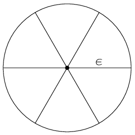
A proof of all but the 4 point case may be found in [8]; we prove the two point case with both zeroes even here. Consider a disk , centered at , of radius in the flat metric given by , where is small enough that contains no other zeroes of . Since is of order , horizontal trajectories will dead-end into . Cut along these to make half-disks, each with a marked point given by half way along the cut. Pick some with . If and are both even, construct two special half-disks by splitting the marked point given by into two marked points apart. Also shift the marked point given by by on the remaining disks, as in Figure 1. The trajectory structures on the individual half-disks do not change, and the half-disks can be glued back together, again as in Figure 1, to give an disk containing zeroes of order , with the same trajectory structure at the boundary as the original . The remaining two and three point cases are proved similarly.
For the case of four zeroes, if any of the are even then we may apply some combination of two and three point surgeries to get the desired result. If are all odd then we cut around into half-disks and glue as in Figure 2. Again, in all of these surgeries we have a choice of both and . ∎

Define to be adjacent to if it is possible to obtain an element in by (possibly repeatedly) applying the surgeries of Lemmas 5.1 and 5.2 to an element in . This puts a poset ordering on , the set of partitions of : we say if there exists a component of that is adjacent to a component of . Note that if is adjacent to , then .
Lemmas 5.1 and 5.2 detail surgeries that allow us to break up zeroes of quadratic differentials; however, again following [3] we may collapse zeroes in the reverse process. We say three points, , and , are co-linear if for a fixed there exist -trajectories between and .
Lemma 5.3.
Suppose is such that there exists a saddle connection between and of length , all other saddle connections from or are of length at least , and are not both odd. Then there exists such that may be obtained from via the surgery of Lemma 5.1.
Suppose is such that there exist saddle connections between and of length , are co-linear, and all saddle connections from are of length at least . Then there exists such that may be obtained from via the surgery of Lemma 5.1.
Proof.
We first prove the two point case. Label the points in each of the two top left disks of Figure 3 by and . For both of the two top left disks are contained in and therefore contain no other zeroes of . Since we may reverse the cutting and pasting process of Lemma 5.1 to obtain . For the three point case, label the points in the the two bottom left discs of Figure 3 by , with in the middle. For contains either of these two discs. Thus these disks contain no other zeroes of and since we may reverse the cutting and pasting of Lemma 5.2 to obtain . ∎


In the next proposition we will construct (square) transpositions of zeroes of by colliding two zeroes to get in an adjacent and then breaking up the newly formed zero of with respect to varying . Breaking up a single zero into two zeroes in this manner gives us a transposition; however, breaking a single zero into three gives us something slightly different. Define a transposition of and mod to be an element of such that follow paths that are not homotopic on , but are homotopic on . If is a path between through we will refer to a transposition of mod along ; by this we mean that and follow small deformations of on opposite sides of . Similarly if we refer to a transposition of along we mean their transposition along a slight deformation of to one side of .
Proposition 5.4.
Proof.
We first prove the proposition for the two point case. Suppose is obtained from by surgering with respect to . Let be the new trajectory between of length . Create a curve by surgering with respect to , . Now, there exists a ball of some radius around the zero of of order containing no other zeroes of , so we apply the surgery of Lemma 5.1 to with respect to some fixed and vary between and either or (depending on whether we transpose or square transpose and ) to get a loop of surfaces, , centered at . intersects at , and we define to be the sub-curve of from to . Then gives us the desired loop in .
Following the same procedure for three points, we get a (square) transposition of mod along the union of the two trajectories between them in . ∎
Proposition 5.4 allows us to create (square) transpositions of various zeroes of a quadratic differential (possibly mod a third zero); however, the (square) transpositions created this way may be based at different elements of . In the next section we show that one way of obtaining elements based at the same is to consider hyperelliptic quadratic differentials.
6 (Square) transpositions in certain strata
In the next two sections we show that there exists a family of for which . We do so by explicitly constructing loops of quadratic differentials corresponding to the generators of ; in this section we construct the necessary (square) transpositions, and in the next section the null and -commutators. For simplicity of notation we refer to the elements we construct as being in ; however, they will be unchanged under .
We say that contains all transpositions between if for all edges between and , or (depending on whether and are of the same weight or not). We say that contains all transpositions if the above is true for all pairs of zeroes of . In Lemmas 6.1 - 6.4 we construct a variety of transpositions in hyperelliptic strata, and in the final proposition of the section we show that for some the transpositions constructed in the four lemmas suffice to generate all transpositions in .
For any hyperelliptic quadratic differential, , we let denote the hyperelliptic involution on and a projection of to . We will use to denote the the projection of to . Notice that any zero of a hyperelliptic quadratic differential at a branch point of must be of even order. Unless specified otherwise we do not assume that the in are distinct.
Lemma 6.1.
Let be a hyperelliptic quadratic differential, and label the zeroes of by . Suppose exactly are at branch points of and at least one of , say , is even. Let be an edge between , , such that . Then contains an element corresponding to the (square) transposition of along . Analogous statements are true for , and .
Sketch of proof.
To prove the lemma we construct paths in the hyperelliptic locus of , from to quadratic differentials with discs that satisfy the conditions of Lemma 5.3 (as in Figure 3), and we then apply Proposition 5.4. In the case where at least one of is even, this proves the lemma. In the case where both and are odd the path we create moves near an even zero, , and we create a (square) transposition of mod . However, since is even we also have a square transposition of and , and the composition of the two gives us the desired (square) transposition of and (see Figure 4). ∎
Proof.
Let , , and let be the projection of to . By abuse of notation we also use to mean the images of under the maps and .
We first assume at least one of is even. Define:
and label the singularities of by , such that for and for . Since any branch zero is of even order, and the number of single poles of is always positive. By Proposition 2.2 we may construct a quadratic differential on with arbitrary zeroes; thus, define to be the quadratic differential with zeroes at . Let be the double cover of , ramified at .
As approaches 1, approaches , and there exists close to 1 such that satisfies the conditions of Lemma 5.3. Then we may apply Proposition 5.4 to obtain a (square) transposition, , of , in , along a trajectory homotopic to . Let be the image of in under . Along and (square) transpose along . Further, follows a trivial path (since ) and all other zeroes stay constant, so this gives us the desired (square) transposition.
Now suppose both and are odd. Let be as above and recall that is even. let be an edge from to such that , and let be the edge between and either or that projects to . Since does not intersect itself , and also by construction .
Define to be the quadratic differential with zeroes at , and let be the double cover of . Again there will be some such that satisfies the conditions of Lemma 5.3. (Some slight deformation of and may be required to get and co-linear). Then by Proposition 5.4, contains a transposition of and mod along . However, since is a zero of even order there exists a square transposition of and along , also in . The composition of this square transposition and the transposition of and mod is shown in Figure 4, and gives a true transposition of and along . The rest of the proof follows as in the even case. ∎


Notice that any geodesic, , between two branch points of a hyperelliptic quadratic differential will have a ‘twin’ geodesic, , parallel and of the same length. We would like to prove a lemma similar to 6.1 for branch zeroes; however, colliding two branch zeroes along will also cause the length of to go to zero and a homology cycle to collapse. We deal with this by leaving the hyperelliptic locus of shortly before colliding the two zeroes, and showing that for a generic element outside the hyperelliptic locus, the trajectories corresponding to and will be of different lengths.
In particular, for any pick and notice that for any loop, on based at and , parallel transport along takes a vector either to or . This gives us a homomorphism:
Following Masur and Zorich in [10], this gives us a double cover of , , endowed with an induced flat metric that by construction has trivial holonomy and thus defines an Abelian differential, on , with zeroes . is the canonical double cover of , and has a natural involution, . Let be the subspace of that is anti-invariant with respect to . Any has a double cover , and we define . We say that are if is homologous to .
We may define a basis for by lifting a basis of , , to the corresponding . Define the period of to be . Notice that locally elements of will have double covers in the same stratum of Abelian differentials, and thus we may identify copies of over nearby surfaces. It is well known that the periods of a basis for give local coordinates on . Thus if and are not omologous, the homology classes of , are independent in , and only on a set of measure zero. Since , the same will be true of and - if they are non-omologous they are of the same length only on a set of measure zero.
Lemma 6.2.
Let and be as in Lemma 6.1, with some odd, at least two branch zeroes, and . Let be a trajectory between two of the branch zeroes of such that the trajectory does not contain any other zeroes of , and let . Then there exists some open set, , containing , such that for almost every element of these trajectories are not of the same length.
Proof.
As noted above, if and are not omologous in then they are generically not of the same length. Thus, to prove the lemma we suppose that is homologous to zero and show a contradiction.
If is homologous to zero then it is a separating curve. Let be the surface with boundary obtained by cutting along , which together form a non-trivial cycle. Since , is connected. If any element of mapped to under then cut at would still be connected, which implies that every element of maps to 1 under . But by assumption one of the zeroes of is odd and a small loop around it will map to under , giving us the desired contradiction. ∎
Now we can prove the analog of Lemma 6.1 for branch zeroes.
Lemma 6.3.
Let , and be as in Lemma 6.1, with at least one odd, and let be any edge between two branch zeroes of , and , . Then contains a (square) transposition of along .
Proof.
Let , , , be the edge between , and let be its projection to . Let and label the zeroes of as . Define to be the element of with zeroes at . Taking a double cover of branched at its last zeroes we get an element of , which we call .
As approaches 1, approaches and all other are fixed. As in Lemma 6.1 we wish to show there exists a subset of some containing and , and satisfying the conditions of Lemma 5.3. In fact, because and are both of even order we may actually relax the conditions of Lemma 5.3: if and are apart it suffices to show that all other saddle connections on are of length greater than . (We see this by proving Lemma 5.3 in the same way but only for the case of two even zeroes, as in the second pair of discs in Figure 3). This condition is not initially satisfied because on there are two short trajectories of the same length running between and . However, Lemma 6.2 implies that there exists arbitrarily close to any such that the trajectories in the homotopy classes of and are of different lengths. Because of the involution on we may assume the trajectory on in the homotopy class of is shorter and thus satisfies the (modified) conditions of Lemma 5.3. Then there exists a (square) transposition of along , based at . The rest of the argument follows as in Lemma 6.1. ∎
Lemma 6.4.
Let and be as in Lemma 6.1, and let be a branch point of that is also a regular point of . Let be an edge between and , , such that . Then is an edge between and , and contains an element corresponding to the transposition of along .
Proof.
Let be a small deformation of to one side of that is still an edge. We can always choose so that and . As in the previous two lemmas, let be a projection of to , with singularities , and let . Define to be the quadratic differential with zeroes at , and let be its double cover. and , is the desired element of . ∎
The previous four lemmas will allow us to show that certain hyperelliptic strata contain all of their transpositions, but first we need one more technical lemma. Recall that the maximal number of faces a planar graph with vertices can have is . (Such a graph will be a triangulation, with edges.) By removing edges from such a graph it is always possible to construct a planar graph with vertices and fewer than faces. (As earlier in the paper, we do not allow graphs to have double edges or loops.)
Lemma 6.5.
Let be a planar graph with vertices and faces, . Then we may associate to each face of a pair of vertices adjacent to the face such that the same pair is not associated to more than 1 face.
Proof.
It suffices to associate a unique adjacent edge to each face of , since this is equivalent to associating the two vertices adjacent to the edge to the face. Pick any face, , of and any edge, , adjacent to . is adjacent to one other face, which we call . has at least two other possible adjacent edges, so again pick any edge to associate to , and let the other face adjacent to . Continue this process until one of two things happens. Either an edge is associated to each face, or at stage for and . In the first case we are done, and in the second the remaining faces of the graph do not have any adjacent edges that have been associated to any other face, so we pick any face, call it and resume the process. ∎
Proposition 6.6.
Suppose that is such that , are all even, and there exists such that . Then for any , contains all transpositions.
Sketch of Proof.
Our plan is to construct a hyperelliptic with higher order zeroes at branch points, and then put a graph on with the single zeroes of at the vertices and at most one higher order zero in each face. We use Lemmas 6.1 and 6.4 to construct the transpositions associated to each edge of the graph, which via Theorem 4.2 gives us all (square) transpositions of single zeroes with each other and with higher order zeroes. We then apply Lemma 6.3 to get (square) transpositions of the higher order zeroes with each other. ∎
Proof.
By Theorem 2.7 is connected so we need not consider connected components. Without loss of generality suppose . Put a graph on with vertices and faces. Since , , and it is always possible to construct such a graph. Mark 2 points in each of faces of , and 3 points in the st. By Proposition 2.2 there exists on such that the vertices of are zeroes of of order , marked points are zeroes of of order , and the remaining marked points are poles of of order 1. Since , has at least 2 poles and we assume the face contains the zero of order and 2 poles. Denote the single zeroes of by . To each face of we associate a pair of vertices as in Lemma 6.5.
Take a double cover of ramified at the marked points in the faces of , minus the zero of order . Assume each branch cut is between two points in the same face and is contained in that face. This gives us . has two copies of embedded into it, and ; denote their vertices by and , with , . By associating a pair of vertices to each face of we have associated a quadruplet of vertices, and , to each of the branch cuts of . Construct a pair of edges, and , between and through the th branch cut, , as in Figure 5. Notice that we may always construct and so that they do not intersect. For the st branch cut, both branch points are regular and we construct edges, and between and , as in Lemma 6.4. gives us a connected graph on with faces and two faces associated to each branch cut. This graph will be a 2-cell embedding and by construction satisfies all of the hypotheses of Theorem 4.2. Exactly one branch point is in each of faces associated to the first branch cuts. For the two faces, and , associated to the st branch cut, so again there is one zero of order in each of .
By Lemma 6.1 we may construct an element of corresponding to the transposition of along both and for . Further, each edge of is contained entirely on one sheet of , so and again by Lemma 6.1 . Lemma 6.4 gives us transpositions associated to and . Consequently for every edge of , . Since there is at most one higher order zero in each face, Theorem 4.2 implies contains all transposition of the zeroes of order 1 with each other, and all square transpositions of zeroes of order 1 with zeroes of order .
Now pick any , and let be its double cover, ramified at the zeroes of not of order 1. Then all of the even zeroes of are at branch points of and by Lemma 6.3 contains all (square) transpositions of zeroes of order with each other. But is isomorphic to so the same is then true for . This proves the proposition. ∎


7 Constructing the remaining generators
We have shown that in some cases all transpositions and square transpositions of zeroes of are contained in . However, for where many but not all points are not of equal weight, Theorem 4.14 and Corollary 4.15 imply that is generated by transpositions, null , and -commutators. In some cases we can again use techniques of colliding and breaking apart points from Section 5 to show that these last two types of elements are in .
Let be standard generators of . Recall that in Sections 3 and 4 we did not explicitly define the , we only stated that one of the generators of must be a loop corresponding to moving around . There are infinitely many choices of such a loop, differing by various products of transpositions.
Lemma 7.1.
Let contain all of its transpositions, and suppose . Further suppose is adjacent to and contains all transpositions of the two newly formed points. Define to all equal 1, and to all equal -1. Then for any , for any choice of , for any such that , , and for any , .


Proof.
To prove the lemma we first explicitly define and show that under our choice of definition, . We then pick any other choice of generators, , any (not necessarily distinct) such that , and any permutation . We define . We show that differs from only by a product of transpositions and is thus also in .
Label the two zeroes of of order as and . For any pick two edges, and , between such that is homotopic to and , as in the left of Figure 6. By assumption . Further, defining and as in the left of Figure 6, is homotopic to . Thus .
Now pick an explicit loop of surfaces in the homotopy class , , such that . Surger every by some continuously varying , possibly multiple times, to get a loop of surfaces , and define . Let be the zeroes of of order formed from the surgery. We may then define to be the path followed by , and so forth (as in the right of Figure 8). Under these definitions of the , , we have created .
Now let be an element of and consider . Since is supported on a subset of that is a disc, it may be written as a product of (square) transpositions. We have assumed contains all transpositions, so and therefore .
Similarly define be a different choice of generators, and define . Again is supported in a disc on and therefore .
Finally suppose we have (not necessarily distinct) such that , , and define . Either and or may be written as a product of two transpositions, as in the first paragraph of this proof. Then the following is in :
As above is supported in a disc and therefore in . This then implies .
A combination of the above implies the lemma for the specific choice of , surgered from . However, since fundamental groups with different base points are isomorphic, the same will be true for any element of . ∎
Lemma 7.1 shows that under certain adjacency conditions it is possible to construct any null involving points of certain weights. When the lemma implies that if contains all of its transpositions, it also contains all null involving two points of equal weights.
Proposition 7.2.
Let and with max, all even, and some . Then for any , all null are contained in .
Proof.
By Theorem 2.7 there is only one connected component of .
Let with the zeroes of of order 1. By Proposition 6.6 contains all of its transpositions; by Lemma 7.1 it contains any , .
For , let and notice that by Lemmas 5.1 and 5.2, (this is not true if ). Since is even there exists a component of , , that contains a hyperelliptic element, , for which both zeroes of order are at branch points. By Lemma 6.3, contains all transpositions of the two zeroes of order , and by Lemma 7.1 it contains each of the null involving only those two zeroes. Therefore Lemma 7.1 implies any null consisting of a single zero of order moving around and zeroes of order 1 moving around is in .
If we let and note that . By the same argument as above there exists such that contains each of the null involving only the two zeroes of order 4. Thus we get the null involving a zero of order and zeroes of order 1 moving one way around , and 4 zeroes of order 1 moving the other. We compose and cancel with null involving points of order 1 to get a null with a zero of order 2 moving around and two zeroes of order 1 moving around .
This gives us any null consisting of a single zero of higher order moving one way around and zeroes of order 1 moving the other. These and the where generate all null . ∎
Notice that there are strata of the form specified in Proposition 6.6 for which there exist null to which Lemma 7.1 does not apply. For example, in we can have a null consisting of the point of order 20 moving one way around and 20 points of order 1 moving the other, but since there are not 20 distinct points of order 1 we cannot collide them to use the technique of Lemma 7.1.
Finally we would like to consider when -commutators are contained in .
Proposition 7.3.
Let , where and the are as in Proposition 7.2. Then for any , any -commutator is in .

Proof.
Let be the zeroes of of weight 1, and the zeroes of weight . where is by assumption is less than , . By Proposition 7.2 contains all of its null . Thus the following is also in :
| (9) |
For and , commutes with . If but then = where is a square transposition of , defined appropriately with respect to . For example, in Figure 7 we have two points going around on a torus and an explicitly defined , with .
Thus if (9) is equal to:
| (10) |
Notice that the maximal value for is , and this implies that for any . The first of the two elements in parentheses in (10) is in the kernel of , so we may apply Corollary 4.6 to show that it can be written as a product of transpositions. Proposition 6.6 says that contains all of its transpositions; thus the element on the left is in . This in turn implies implies .
If then (9) is equal to (10) except that the first element in parentheses will contain some additional ’s. However it will still be in the kernel of and again .
Similarly, for a zero of higher order and an edge between , we would like to show that is in , so we consider the following:
By assumption both and the elements in parentheses are in , so the whole element is. Since commutes with , commuting the as in (10) gives us the desired result.
Finally, any product of square transpositions of two higher order zeroes is contained in by Proposition 6.6, because it is a product of transpositions. This covers all possible generators of . ∎
8 Conclusion
We summarize by answering the question of when is equal to .
Theorem 8.1.
Let with max, all even, and some . Then .
Proof.
In [2], Copeland shows a similar result for and . His techniques are somewhat different and rely on the fact that in the top stratum one may interpolate two quadratic differentials and expect the result to be in the same stratum.
Thus, for certain we have constructed . Of course, we are actually interested in and would thus like to determine the kernel of . However, it may be difficult to say anything about this kernel.
For example, let . and are both smooth connected complex varieties and is a dominant morphism of varieties. A fiber of is a copy of with a codimension 1 subset removed, so it is connected and has at least one smooth point.
Then there is a non-empty Zariski open set such that is a fibration (see [11], for example), and for a generic fiber, , of we have the following short exact sequence:
Similarly consider the projection given by . Again, both and are connected, smooth, complex varieties and is a dominant morphism. Further, notice that . In other words, the fibers of may be viewed as a codimension subset of the fibers of . Thus the fibers of are also all connected, containing at least one smooth point, and for a generic fiber, , of , we again have the SES:
Since is simply connected, is isomorphic to the fundamental group of a generic fiber of . (One would expect similar arguments apply to any such that a generic fiber of is connected - for example any of Theorem 2.7).
If a generic fiber of were also a generic fiber of then we would have and the kernel of would, in fact, be trivial. However, it is possible that this is not the case, and in general considering the fundamental groups of specific, possibly singular, fibers of seems to be difficult. Again for , for example, these fibers correspond to the complement of discriminant hypersurfaces in and there is a great deal of literature on the subject, but very little dealing with arbitrarily singular fibers.
Acknowledgments: I would like to thank P. Seidel, H. Masur, and especially J. Copeland for illuminating conversations and helpful comments.
References
- [1] J. Birman. Braids, Links and Mapping Class Groups. Annals of Mathematics Studies, no. 82, Princeton University Press, 1974.
- [2] D.J. Copeland. Monodromy of the Hitchin Map over Hyperelliptic Curves. Int. Math. Res. Not. 2005, no. 29, 1743-1785.
- [3] A. Eskin, H. Masur, A. Zorich. Moduli Spaces of Abelian Differentials: The Principal Boundary, Counting Problems and the Siegel-Veech Constants. Publ. Math. Inst. Hautes Etudes Sci. No. 97 (2003), 61-179.
- [4] E. Fadell, L. Neuwirth. Configuration Spaces. Math. Scand. 10 (1962), 111-118.
- [5] M. Kontsevich, A. Zorich. Connected Components of the Moduli Spaces of Abelian Differentials with Prescribed Singularities. Invent. Math. 153 (2003), no. 3, 631-678.
- [6] M. Kontsevich, A. Zorich. Lyupanov Exponents and Hodge Theory. Preprint IHES M/97/13, 1-16 electronic version: hep-th/9701164.
- [7] H. Kronk, R. Ringeisen, A. White. On the 2-cell imbeddings of complete n-partite graphs. Colloq. Math. 36 (1976).
- [8] E. Lanneau. Hyperelliptic Components of the Moduli Spaces of Quadratic Differentials with Prescribed Singularities. Comment. Math. Helv. 79 (2004), no. 3, 471–501.
- [9] H. Masur, S. Tabachnikov. Flat structures and rational billiards, in Handbook of Dynamical Systems, Vol. 1A, 1015-1089.
- [10] H. Masur, A. Zorich. Multiple Saddle Connections on Flat Surfaces and the Principal Boundary of the Moduli Space of Quadratic Differentials. Preprint: Arxiv:math.GT/0402197
- [11] M. Nori. Zariski’s Conjecture and Related Problems. Ann. scient. Ec. Norm. Sup., ser. 4, no. 16, 1983, 305-344.
- [12] G.P. Scott. Braid Groups and the Group of Homeomorphisms of a Surface. Proc. Camb. Phil. Soc., 68 (1970), 605-617.
- [13] K. Strebel. Quadratic Differentials. Ergeb. Math. Grenzgeb. 3:5, Springer-Verlag, 1984.
- [14] W. Veech. Moduli spaces of quadratic differentials. Journal d’Analyse Math. 55 (1990), 117-171.
- [15] K. Walker Connected components of strata of quadratic differentials over Teichmuller space. ArXiv: