Impurity in a granular gas under nonlinear Couette flow
Abstract
We study in this work the transport properties of an impurity immersed in a granular gas under stationary nonlinear Couette flow. The starting point is a kinetic model for low-density granular mixtures recently proposed by the authors [Vega Reyes F et al. 2007 Phys. Rev. E 75 061306]. Two routes have been considered. First, a hydrodynamic or normal solution is found by exploiting a formal mapping between the kinetic equations for the gas particles and for the impurity. We show that the transport properties of the impurity are characterized by the ratio between the temperatures of the impurity and gas particles and by five generalized transport coefficients: three related to the momentum flux (a nonlinear shear viscosity and two normal stress differences) and two related to the heat flux (a nonlinear thermal conductivity and a cross coefficient measuring a component of the heat flux orthogonal to the thermal gradient). Second, by means of a Monte Carlo simulation method we numerically solve the kinetic equations and show that our hydrodynamic solution is valid in the bulk of the fluid when realistic boundary conditions are used. Furthermore, the hydrodynamic solution applies to arbitrarily (inside the continuum regime) large values of the shear rate, of the inelasticity, and of the rest of parameters of the system. Preliminary simulation results of the true Boltzmann description show the reliability of the nonlinear hydrodynamic solution of the kinetic model. This shows again the validity of a hydrodynamic description for granular flows, even under extreme conditions, beyond the Navier–Stokes domain.
Keywords:
granular matter, kinetic theory of gases and liquids, rheology and transport propertiesI Introduction
The understanding of transport processes occurring in granular mixtures is still challenging. In the low- and moderate-density regimes the Boltzmann and Enskog equations, suitably adapted to account for inelastic collisions, have proven to provide an adequate framework for the study of granular flows [1, 2]. In particular, if the spatial gradients present in the system are weak, the Navier–Stokes (NS) constitutive equations for the fluxes of mass, momentum, and energy have been derived (with explicit expressions for the transport coefficients) for the model of inelastic hard spheres characterized by constant coefficients of normal restitution . Most of the early derivations were restricted to the quasielastic limit (), thus assuming an expansion around Maxwellians at the same temperature [3, 4, 5, 6, 7, 8]. However, the nonequipartition of energy becomes significant beyond the quasi-elastic limit, as confirmed by kinetic theory [9, 10, 11, 12], computer simulations [11, 13, 14, 15, 16, 17, 18, 19, 20, 21], and real experiments [21, 22, 23]. A more realistic derivation of the NS transport coefficients [24, 25, 26, 27] requires taking into account the nonequipartition of energy and applies for finite dissipation. The accuracy of this latter approach has been confirmed by computer simulations in the cases of the diffusion [28, 29] and shear viscosity [30, 31] coefficients. On the other hand, the practical applicability of the NS equations is limited to small spatial gradients, while many steady granular flows do not fulfill in general this condition, due to the coupling between inelasticity and gradients [1, 32].
The physical situation we study in this work corresponds to a gas of inelastic hard spheres enclosed between two parallel walls at moving with velocities along the -axis and kept, in general, at different temperatures [33, 34, 35, 36, 37, 38]. In the base steady state the flow velocity is along the -axis and the hydrodynamic fields depend on the variable only (planar Couette flow). This macroscopic state is characterized by a combined momentum and heat transport described by the pressure tensor and the heat flux , respectively. A sketch of the geometry of the steady planar Couette flow for the symmetric choice is given in Fig. 1.
Since granular matter is generally present in polydisperse form, the study of the Couette flow in the case of a granular mixture is an interesting problem from a fundamental and practical point of view. Needless to say, the general problem is quite intricate since, not only the number of parameters (masses, sizes, composition, and coefficients of restitution) but also the number of transport coefficients are higher than in the monocomponent case. As a first step and to gain some insight into the general problem, in this paper we consider the tracer limit case, namely a binary mixture where the mole fraction of one of the components (tracer species, denoted by the label 1) is much smaller than that of the other component (excess species, denoted by the label 2). In this tracer limit, the state of the excess species is unaffected by the presence of the tracer particles and so its velocity distribution function obeys a closed Boltzmann equation in the low-density regime. In addition, the mutual collisions among the tracer particles can be neglected versus the tracer-gas collisions, so that the tracer velocity distribution function obeys a linear (inelastic) Boltzmann–Lorentz equation. This problem is formally equivalent to that of an impurity or intruder immersed in a granular gas, and this will be the terminology used in this paper. Since the impurity particle is assumed to be mechanically different from the gas particles, the dimensionless parameters characterizing the mixture are the coefficients of restitution and , the mass ratio , and the size ratio .

Unfortunately, the complexity of the nonlinear Couette flow makes its treatment at the level of the Boltzmann equation practically unattainable, even in the monocomponent case. Thus, here we will consider a model kinetic equation recently proposed for granular mixtures [39]. In the tracer limit, this kinetic model reduces to the same closed kinetic equation for the excess species as considered in Ref. [37] plus a Boltzmann–Lorentz-like kinetic equation for the impurity particle. The kinetic equation for admits an exact solution for the steady planar Couette flow [37]. Exploiting the formal analogy between the kinetic equations for and , we find in this paper an exact solution for . This solution allows us to obtain the most relevant velocity moments of , which are directly related to the momentum and heat fluxes associated with the impurity. In particular, as expected, the impurity temperature clearly differs from the granular temperature of the gas particles, showing again the breakdown of the energy equipartition in nonequilibrium states.
The exact solution found here qualifies as a “normal” or hydrodynamic solution since and depend on space only through an explicit functional dependence on the hydrodynamic fields. This hydrodynamic description applies even at strong dissipation (i.e., beyond the quasi-elastic limit) and strong inhomogeneity (i.e., beyond the NS domain), as long as the densest regions of the system remain sufficiently dilute and the molecular chaos assumption holds. This provides a counter-example against the speculation that a hydrodynamic description for granular flows is limited to weak dissipation and/or weak inhomogeneities. In order to assess the reliability of this hydrodynamic solution, we have also solved the model kinetic equation by means of Monte Carlo simulations with Couette-flow boundary conditions. Comparison with the hydrodynamic solution shows that the latter is not a mathematical artifact but applies in the bulk region of the system, where boundary effects are negligible. This agreement between theory and simulations holds for system sizes as small as a few mean free paths.
In order to gain some insight into the expected hydrodynamic fields in the Couette problem, let us consider first a monocomponent granular gas. In this case, the exact energy and momentum balance equations yield
| (1) |
| (2) |
| (3) |
where and 3 for hard disks and spheres, respectively, is the number density, and is the cooling rate due to the inelastic character of collisions. By dimensional analysis in the dilute limit, , where is an effective collision frequency for hard spheres. Equations (1)–(3) do not constitute a closed set of equations for the hydrodynamic fields , , and , unless the constitutive equations expressing the fluxes as functionals of the hydrodynamic fields are known. For illustration, let us assume for the moment that the hydrodynamic gradients are small enough as to justify the use of the NS constitutive equations. Due to the geometry of the problem, at NS order we have [40, 41], from which, with (3), it immediately follows that the hydrostatic pressure is constant, i.e.,
| (4) |
Moreover, the NS constitutive equations imply that and
| (5) |
where is the shear viscosity, is the thermal conductivity ( being the mass of a particle), and is a transport coefficient absent in the elastic case (). The explicit form of the dimensionless functions , , , and is known [40, 41]. Insertion of Eqs. (4) and (5) into Eqs. (1) and (2) yield
| (6) |
| (7) |
Therefore, according to the NS description, the local shear rate scaled with the local collision frequency is a constant, and the temperature profile is such that is a constant that depends on the reduced shear rate and the coefficient of restitution . The set of NS base steady states in the system have been analytically solved in a recent work [42].
As said before, due to inelasticity these steady states do not have small spatial gradients (except for [42]) and thus a kinetic description beyond the NS domain is in general required in order to properly describe granular Couette flows. Specifically, this is even more necessary if (and this happens when the viscous heating dominates over collisional cooling [32]), since in this case the Knudsen number is always greater than the one for [42]. Such a description of the Couette flow beyond the NS domain was carried out in Ref. [37] for a monocomponent granular gas with . Interestingly enough, this solution shares with the NS description the structure of the hydrodynamic profiles (4), (6), and (7). However, in the constitutive equations, the transport coefficients and the parameter are nonlinear functions of the shear rate [37]. At the same time, the solution is also able to capture normal stress differences () and the component of the heat flux along the flow direction (), which are all nonlinear effects [37]. All theoretical results in Ref. [37] compare well with Monte Carlo simulations of the Boltzmann equation, showing the reliability of the kinetic model beyond the quasi-elastic limit. As an illustrative example of the necessity of a nonlinear description, we briefly analyze the case , which occurs for a threshold value of that in the NS description is and in the nonlinear Couette flow is [37]. We show in Fig. 2 the disagreement between both values, which becomes very apparent for values far from the quasielastic limit. As shown in Ref. [37], the nonlinear prediction agrees very well with Monte Carlo simulations of the Boltzmann equation.
We propose in this work a theoretical solution of the nonlinear hydrodynamic profiles for the impurity that exhibits absence of mutual diffusion (i.e, flow velocities are equal for impurity and excess components). Furthermore, this solution for the impurity also obeys equations of the form (4), (6), and (7). We will use a numerical solution of the kinetic equation by a Monte Carlo method in order to show that the theoretical solution we propose matches the hydrodynamic profiles and transport coefficients that result from the kinetic equation. Furthermore, with the use of the numerical solution we show that the hypotheses, notably the absence of mutual diffusion, used in order to find our hydrodynamic solution are actually always true in a wide range of system parameters (including shear rate and inelasticity). In addition, we present preliminary Monte Carlo simulations of the Boltzmann equations which confirm the hydrodynamic profiles predicted by the nonlinear hydrodynamic solution of the kinetic model.

This paper is organized as follows. The kinetic model for the mixture is described in Sec. II. Then, the physical problem we are interested in is introduced. Section III presents the exact hydrodynamic solution to the kinetic equations for and , with explicit expressions for the heat and momentum fluxes of both species. The simulation method is described in Sec. IV and comparisons between the theoretical predictions and the simulation results is carried out in Sec. V. Finally, the results are summarized and discussed in Sec. VI.
II Kinetic model for granular mixtures
Let us consider a mixture composed by smooth inelastic disks () or spheres () of masses and diameters , the inelasticity of collisions between a sphere of species and a sphere of species being characterized by a constant coefficient of restitution . We will focus on the dilute limit, i.e., the mean free path of the particles is much larger than their sizes. The relevant hydrodynamic fields are the number densities , the flow velocity , and the temperature . They are defined in terms of moments of the velocity distribution functions as
| (8) |
| (9) |
| (10) |
where is the peculiar velocity, is the total number density, is the total mass density, and is the pressure. Furthermore, the second equality of Eq. (9) and the third equality of Eq. (10) define the flow velocity and the partial kinetic temperature for each species, respectively. In addition, in the dilute limit the pressure tensor and the heat flux associated with species are given by
| (11) |
In the low-density regime the distribution functions obey a set of coupled nonlinear Boltzmann equations [24]:
| (12) |
where denotes the inelastic Boltzmann operator that gives the rate of change of due to collisions with particles of species . It is given by
| (13) | |||||
In Eq. (13), is the dimensionality of the system, , is a unit vector along the line of centers, is the Heaviside step function, and is the relative velocity. The primes on the velocities denote the initial values that lead to following a binary (restituting) collision:
| (14a) | |||
| (14b) |
where , so that .
However, due to the mathematical complexity of the Boltzmann equation, and in order to describe general nonequilibrium states, it is useful to replace the Boltzmann collision operator with a more tractable model operator that reproduces the collisional transfers of mass, momentum, and energy of the true inelastic Boltzmann operator, namely
| (15) |
Extending the model proposed by Brey et al. [43] for the monocomponent case and enforcing Eq. (15) in the Gaussian approximation, we have recently proposed the following model kinetic equation for inelastic mixtures [39]:
| (16) |
where
| (17) |
is a velocity-independent effective collision frequency of a particle of species with particles of species ,
| (18) |
is the contribution to the cooling rate of species due to the inelastic collisions with particles of species , and
| (19) |
is a reference distribution function. In the above equations,
| (20) |
| (21) |
| (22) |
We now specialize to the problem analyzed in this paper, namely a binary mixture where one of the species () is present in tracer concentration (). In this case, Eqs. (9) and (10) imply that and . In addition, the mixture is subjected to the steady Couette flow (see Fig. 1), so that the spatial dependence of all the quantities is limited to the variable. In the tracer limit, the state of the excess component () is not disturbed by the presence of the impurity and so Eq. (16) for becomes
| (23) |
where, according to Eqs. (17)–(22), , , and are given by
| (24) |
| (25) |
| (26) |
Taking moments in Eq. (23), one gets the balance equations of momentum and energy in the steady state:
| (27) |
| (28) |
Since the impurity only collides with particles of the host gas, Eq. (16) for reduces to
| (29) |
where
| (30) |
and , , and are defined by Eqs. (17)–(22) with . The kinetic equations (23) and (29) must be supplemented by appropriate boundary conditions representing the relative motion of the plates at .
The main advantage of the tracer limit is that obeys a closed (inelastic) kinetic equation (the same equation as the monocomponent granular gas). Once solved, the moments , , and can be inserted into Eq. (29) to get a closed equation for . Despite the simplicity of the kinetic model with respect to the original Boltzmann equation, the search for an exact solution to the nonlinear Couette flow problem is a formidable task. In the case of a monocomponent gas, an exact hydrodynamic solution was found in Ref. [37]. Of course, this solution holds for the kinetic equation (23) of the excess component. Based on this solution, in the next section we obtain an exact hydrodynamic solution for the kinetic equation (29) of the impurity.
III Hydrodynamic solution beyond Navier–Stokes order
III.1 Excess component
As said before, an exact solution to (23) was found in Ref. [37]. Such a solution is characterized by the following hydrodynamic profiles:
| (31) |
| (32) |
| (33) |
where is a dimensionless nonlinear function of the shear rate and the coefficient of restitution . This quantity (henceforth called thermal curvature coefficient) characterizes the curvature of the temperature profile as a consequence of both the viscous heating and the collisional cooling. The form of the profiles (31)–(33) coincides with the profiles (4), (6), and (7) predicted by the NS description, except that the thermal curvature coefficient differs from its NS value and is determined consistently, as shown below. The solution to Eqs. (32) and (33) is
| (34) |
where the scaled variable is defined as
| (35) |
and is an arbitrary constant that vanishes if the two wall temperatures are equal but is nonzero otherwise () [42].
For convenience, we refer the velocities of the particles to the Lagrangian frame moving with velocity . In this frame, Eq. (23) can be rewritten as
| (36) |
where
| (37) |
and the derivative is taken at constant . Note that the dependence of the reference distribution on both and is explicit. Taking this into account, the hydrodynamic solution to Eq. (36) is [37]
| (38) |
where
| (39) |
The action of the operators and on an arbitrary function is
| (40) |
respectively. The solution (38) clearly adopts the form of a hydrodynamic or normal solution since its spatial dependence only occurs through a functional dependence on the hydrodynamic fields , , and . This provides a neat example of the existence of normal solutions beyond the NS domain. The solution (38) depends parametrically on the shear rate , the coefficient of restitution and the thermal curvature coefficient . However, only the two first parameters are independent since, as indicated by the notation in Eq. (33), is a nonlinear function of and . The parameter is determined by imposing the consistency conditions
| (41) |
While the first two conditions are identically satisfied regardless of the value of , the third condition in (41) leads to the following implicit equation [44]
| (42) |
Here, we have introduced the mathematical functions
| (43) |
where is the complementary error function and
| (45) |
The representation (42) exists only for or, equivalently, for , where, as discussed in the Introduction, the threshold value of the shear rate corresponds to . In this case, [see the appendix] and so
| (46) |
In the case the viscous heating is exactly balanced by collisional cooling. This state corresponds with the well-known simple shear flow [if in (34)] but also to a non-uniform steady flow (for ) that has been reported recently [42].
Once the parameter is obtained from Eq. (42), the velocity distribution function is completely determined from Eq. (38). Its relevant moments provide the momentum and heat fluxes. The nonzero elements of the pressure tensor are given by [37]
| (47) |
| (48) |
| (49) |
| (50) |
The requirement is equivalent to the consistency condition (42). Equation (50) strongly differs from Newton’s shearing law [see Eq. (5)] since the quantity enclosed by square brackets in Eq. (50) is a highly nonlinear function of the shear rate through the thermal curvature coefficient . For instance, at and the magnitude of is about half its Newtonian value.
Next, we consider the heat flux components and . The latter can be easily determined in terms of making use of the energy balance equation (28), according to which is linear in . Consequently, one gets
| (51) |
where we have taken into account that is also linear in [see Eq. (34)]. Equation (51) can be seen as a generalized Fourier’s law in the sense that is proportional to the thermal gradient with an effective thermal conductivity that is a nonlinear function of the shear rate. The evaluation of the component is much more involved. Multiplying both sides of Eq. (38) by and integrating over velocity, one gets [37]
| (52) |
where we have called
| (53) |
| (54) |
Here,
| (55) |
| (56) |
The existence of a component of the heat flux orthogonal to the thermal gradient and parallel to the flow direction goes beyond Fourier’s law. In fact, is at least of order and so Eq. (52) can be seen as a generalized Burnett effect.
III.2 Impurity particle
Once the hydrodynamic state of the excess component has been characterized, we next want to analyze the hydrodynamic state of the impurity particle.
First, some useful information can be extracted by taking moments in Eq. (29):
| (57) |
| (58) |
| (59) |
Next, we guess (to be confirmed later) that the hydrodynamic state of the impurity is enslaved to that of the granular gas in the sense that
-
(i) there is no mutual diffusion, i.e., ,
-
(ii) the mole fraction is uniform, and
-
(iii) the temperature ratio is also uniform.
The latter parameter must be a function of the mass and size ratios
| (60) |
the reduced shear rate , and the coefficients of restitution and . Of course, the temperature ratio is when the impurity is mechanically equivalent to the gas particles (, ). Taking into account assumption (i), Eqs. (58) and (59) become
| (61) |
| (62) |
Furthermore, assumptions (ii) and (iii) imply that the product and the ratios , , and are constant quantities. The three latter are given by
| (63) |
| (64) |
| (65) |
From a formal point of view, the kinetic equation (23) becomes Eq. (29) by making the changes , , and . The formal change implies the changes , , and . It is then convenient to introduce the auxiliary quantities
| (66) |
| (67) |
Equations (66) and (67), along with , define the profiles of the fields characterizing the distribution function .
The formal mapping described above allows us to easily get the moments of from comparison with those of . In particular, the two first self-consistency conditions are verified, namely
| (68) |
regardless of the values of and . The third self-consistency condition reads
| (69) |
This condition determines the temperature ratio . To evaluate the left-hand side of Eq. (69), it is convenient to obtain first the nonzero elements of the partial pressure tensor . Taking into account Eqs. (47)–(50), one gets
| (70) |
| (71) |
| (72) |
| (73) |
where the functions and are defined by Eqs. (43) and (III.1), respectively. Condition (69) is equivalent to , yielding
| (74) |
For given values of the reduced shear rate and the mechanical parameters of the system (, , , and ), Eq. (74), complemented with Eq. (42) and the relations (63)–(67), becomes a nonlinear closed equation for the temperature ratio , which must be solved numerically. In the case of mechanically equivalent particles, Eq. (74) yields and is equivalent to Eq. (42). Insertion of this solution into Eqs. (70)–(73) gives the elements of the pressure tensor .
III.3 Generalized transport coefficients for the impurity particle
In order to characterize the momentum and heat transport associated with the impurity particle we introduce five generalized transport coefficients. The shear stress defines a (dimensionless) nonlinear shear viscosity coefficient as
| (77) |
The anisotropy of the normal stresses can be measured through the viscometric coefficients and :
| (78) |
The heat flux defines a generalized thermal conductivity coefficient and a cross coefficient as
| (79) |
From Eqs. (70)–(73), (75), and (76) it is possible to identify the expressions for these five generalized transport coefficients. They are given by
| (80) |
| (81) |
| (82) |
| (83) |
| (84) |
Their expressions in the limit are explicitly given in the appendix.
IV Monte Carlo simulations
As said before, the exact solution to the kinetic equation (29) derived in Sec. III defines a normal or hydrodynamic solution where its spatial dependence only occurs through the hydrodynamic fields (, , , and ) and their gradients. This solution is free from boundary-layer effects and formally corresponds to idealized boundary conditions of infinitely cold walls (). For more details the reader is referred to Appendix B of Ref. [37]. The important point is whether or not this exact solution actually describes the steady state reached by the system, in the bulk domain, when subject to realistic boundary conditions and for arbitrary initial conditions. To confirm this expectation, one needs to solve numerically the set of time-dependent kinetic equations
| (85) |
These equations are solved with boundary conditions at compatible with the wall values and and starting from an arbitrary initial condition. Specifically, we have considered Maxwellian diffuse boundary conditions [37, 45] and an initial distribution of total equilibrium. The latter choice does not imply a loss of generality in the base steady states that are achieved in the system and only affects the transient evolution. Both species are let to simultaneously evolve from the initial state. It is also to be noticed that in the numerical solution of Eq. (85) there is no a priori assumption of equal flow velocities for the two components. i.e., eventual steady-state solutions with are let to occur. However, as we will show, this actually never happens and all the steady states found are consistent with (absence of diffusion).
In this paper we have employed a direct simulation Monte Carlo (DSMC) method [46, 47] to numerically solve the kinetic equations (85) in the three-dimensional case. The DSMC method has been extensively used to solve kinetic equations like the Boltzmann and BGK equations and it has proven to accurately describe transport phenomena in elastic gases and has also successfully been extended to flows in granular gases. In the DSMC method two steps are taken every time interval : the free streaming step, during which a particle with velocity is drifted by and the boundary conditions are applied to those particles leaving the system, and the collision step, in which collision pairs are randomly selected among neighbor particles, being the characteristic collision frequency in the kinetic equation. Our method differs from the elastic case in the addition, in the free streaming step, of the drag term which mimics the inelasticity in the collisions.
The distributions are represented by particles with velocities and positions , . The system is split into layers of width . The particles with positions belonging in layer define the densities , the flow velocities , and the temperatures of that layer. From those quantities one can evaluate and . The free streaming and the collision steps are briefly described below.
IV.1 Free streaming
In the free streaming step the positions and velocities for both components are updated with the following rules:
| (86) |
where is the layer the particle belongs in. The spatial and velocity updates (86) are valid as long as the particle does not leave the system, i.e., . Otherwise, the particle is reentered by applying thermal boundary conditions. If the particle “crosses” a wall, then
| (87) |
where the velocity components are randomly picked from Maxwell distribution functions (at a temperature ) whereas (upper and lower signs for top and bottom wall collision, respectively) with being a random velocity sampled from the Rayleigh probability distribution
| (88) |
The new position after wall collision is
| (89) |
IV.2 Collision step
For each layer a number of particles is randomly selected among those belonging in the layer. Then the velocity of each one of those particles is replaced by
| (90) |
where is a random velocity sampled from a Maxwell probability distribution, with temperatures and for species and , respectively.
IV.3 Time and length scales and simulation technical facts
In the simulations, the quantities are reduced using and as length and time units, respectively, where
| (91) |
and being the average density of the gas particles and a reference thermal velocity, respectively.
Since the aim of DSMC simulations is to solve a kinetic equation, it must be able to describe the dynamical processes occurring in the system at a microscopic level [46]. This means that the width layer must be small compared to the typical microscopic length scale, determined by the mean free path . Similarly, the time step must be small compared to the inverse of the collision frequency, . Also, for obtaining an ergodic simulation, the number of simulated particles must be sufficiently large. We therefore have performed simulations, for both species, with particles, , and . In order to probe a nonlinear Couette flow with (), we have taken a wall velocity difference and a system size typically in the range –, which produces sufficiently large values of .
Taking into account that the relation between microscopic over hydrodynamic scales is given by the Knudsen number Kn, the bin we pick for measurements of the hydrodynamic profiles, including transport coefficients, is of the order of (note that, in our system, the reduced local shear rate is the reference measure for the Knudsen number). This means that the measurements of the hydrodynamic properties are performed over sets of microscopic cells, i.e., an average over microscopic cells is taken for each set (macroscopic cell). In this way, the fluctuations of macroscopic magnitudes, typical in DSMC simulations, are greatly reduced and profiles are smoothed with no loss of resolution at a hydrodynamic scale. Prior to averaging over sets of cells, the hydrodynamic quantities and fluxes are obtained for each cell, by using the expressions that may be found in Ref. [45].
As already explained in Secs. I and III, the reduced shear rate and the thermal curvature coefficient are fundamental quantities in the problem. We measured these quantities by fitting the velocity and temperature profiles from the simulations to fourth-degree polynomials and extracting from these fits the derivatives appearing in the expressions (32) and (33).
An important point in DSMC simulations is the quality of the random number generator. We used for this purpose random generators from Intel MKL 9.1 [48], whose performance has been rigorously examined in technical tests. The DSMC code was written in C language and compiled with Intel C++ 10.0 compiler and run in 64-bit Linux machines.
V Results




V.1 Enslaving of the impurity
The DSMC simulations described in the preceding section show that the steady state reached by the system is in agreement with the bulk profiles assumed in the hydrodynamic solution worked out in Sec. III, i.e., the pressure , the local shear rate , and the local thermal curvature are practically uniform. Moreover, the impurity properties are enslaved to those of the gas particles, namely the system evolves to , , and , in agreement with assumptions (i)–(iii) listed below Eq. (59). As an illustration, Fig. 3 shows simulation data of the pressure and velocity profiles for both the impurity and the gas particles at and .
V.2 Thermal curvature coefficient
In the remainder of this section we compare the theoretical results derived in Sec. III for with the data obtained from our DSMC simulations. Before considering properties associated with the impurity, we first compare the shear rate dependence of the thermal curvature coefficient . Figure 4 displays versus for three values of the coefficient of restitution : (elastic case), (moderately inelastic case), and (quite inelastic case). It is observed that the theory compares well with the simulation results for the three values of considered, even for strongly sheared gases. This confirms the reliability of a (non-Newtonian) hydrodynamic description for granular gases in the bulk domain and beyond the quasi-elastic limit, at least within the framework of the model kinetic equations used. It is apparent from Fig. 4 that, at a given value of the reduced shear rate , the value of decreases with increasing dissipation. This can be qualitatively understood by the tendency of the collisional cooling to produce a concave temperature profile, while the viscous heating tends to produce a convex profile. In fact, both tendencies cancel each other at the threshold shear rate , where . The corresponding values for and , are and , respectively. As noted above, our analytical solution is not mathematically well defined for negative values of (i.e., , shaded region in Fig. 2). This restriction obviously does not apply to the simulations, which can reach states with . These states also include those in the absence of shearing (). States with are interesting and some cases have been studied, in the framework of the NS description and/or in the quasi-elastic limit [49].
V.3 Temperature ratio
Let us study now the main properties characterizing the hydrodynamic state of the impurity. The parameter space of the problem is made of four (dimensionless) material quantities (the mass ratio , the size ratio , and the coefficients of restitution and ) plus the reduced shear rate . For the sake of illustration, we will assume a common coefficient of restitution and a common size (), so that the parameter space becomes three-dimensional. Furthermore, we focus on three values of (, , and ) and three values of (, , and ), so that we consider nine different systems. For each one, we analyze the dependence of the properties of the impurity on the shear rate. Note that, since and , in the case the impurity is mechanically equivalent to the gas particles.
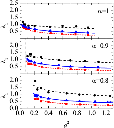
First, the breakdown of energy equipartition, as measured by the temperature ratio , is plotted in Fig. 5. A good agreement between theory and simulations is observed. The lack of energy equipartition is expected because of two reasons. On the one hand, the state of the system is far from equilibrium due to the shearing and thus even in the elastic case () [50, 51]. On the other hand, even in the homogeneous cooling state, the inelasticity drives the system out of equilibrium and, consequently, [10]. We see from Fig. 5 that the impurity has a higher (lower) granular temperature than the gas if it is heavier (lighter) than a gas particle. This agrees with the general trend observed in experiments [22, 23]. Figure 5 also shows that, for a given value of , the deviation of the temperature ratio from unity increases as the shear rate increases. Similarly, at a given value of , the deviation becomes more important with increasing dissipation.
V.4 Generalized transport coefficients
Next, we explore the momentum and heat transport of the impurity, as measured by the rheological quantities , , , , and defined by Eqs. (77)–(79). Figures 6–8 display the three transport coefficients associated with the pressure tensor. As in the case of , the agreement between the theoretical predictions and the simulation results is very good. It is apparent that, regardless of the value of , shear thinning effects are present, i.e., the nonlinear shear viscosity decreases with increasing shear rate. Regarding the influence of the mass ratio, we observe that, for fixed values of and , increases as the mass ratio increases. The influence of dissipation on is smaller than that of . In any case, although hardly apparent in Fig. 6, the value of increases as decreases at given and . It is interesting to note that the ratio is practically independent of , although it exhibits a weak dependence on .
The viscometric coefficients and , which measure normal stress differences, are plotted in Figs. 7 and 8, respectively. The shearing produces a strong anisotropy in the normal stresses: . As expected, this anisotropy increases with the shear rate. While, for given and , the coefficient increases as the impurity becomes heavier, the opposite happens with the coefficient . With respect to the influence of , it turns out that it is practically negligible in the case of , while decreases significantly as the system becomes more inelastic.
Finally, the two transport coefficients and measuring the heat flux are plotted in Figs. 9 and 10, respectively. These coefficients are quite difficult to measure in the simulations near the threshold shear rate , since there the thermal gradient is very small. This explains the scatter of the simulation data near . Again, theory compares quite well with simulations. This is rather satisfactory especially in the case of since this cross coefficient measures complex coupling effects between the velocity and temperature gradients, which are absent in the NS regime. Figure 9 shows that, analogously to what happens with , the generalized thermal conductivity decreases with increasing shear rate. In contrast, the cross coefficient has a non-monotonic dependence for small inelasticities. In agreement with the behavior found for and , both coefficients and decrease as the mass of the impurity decreases, at given values of and . As for the influence of , the results show that and increase with increasing dissipation, this effect being more important for a heavy impurity than for a light impurity. We have observed that the influence of the mass ratio on and is significantly inhibited when one considers the ratios and , especially in the former case. A remarkable counter-intuitive feature is that the coefficient can turn out to be larger than for sufficiently large shear rate. This effect is more notorious as the system becomes more inelastic and/or the impurity becomes heavier. In fact, in the cases and with , one has for any shear rate larger than . Taking into account the definitions (79), the situation implies that , i.e., the shearing induces a heat flux with a component orthogonal to the thermal gradient that is larger than the component parallel to the gradient.
V.5 Preliminary DSMC results from the true Boltzmann equation
Thus far we have shown that the numerical solutions of the model kinetic equations (85) with realistic boundary conditions support the steady-state hydrodynamic solution derived in this paper for the same model beyond the small Knudsen number limit. However, the important question is whether or not such a generalized hydrodynamic description is supported by the more fundamental Boltzmann equation. Comparison between DSMC simulations of the Boltzmann equation and the hydrodynamic solution of the kinetic model shows that the answer is affirmative in the case of a monocomponent granular gas [37].
When an impurity particle is embedded in the host granular gas, the crucial point of the hydrodynamic solution worked out in section III is the enslaving of the hydrodynamic fields of the impurity to those of the bath, as expressed by assumptions (i)–(iii) below Eq. (59). We have performed preliminary DSMC simulations of the Boltzmann equation for the host gas and the coupled Boltzmann–Lorentz equation for the impurity particle and have observed that the properties (i)–(iii) are indeed satisfied in the steady state and in the bulk domain. As an illustrative example, Fig. 11 shows the pressure and velocity profiles, as obtained from DSMC simulations of the Boltzmann equation, for a system similar to that of Fig. 3 but with a larger separation between the plates. Again, in the steady state (and also practically during the transient regime) one has . Moreover, both and are practically constant in the bulk region. As in Fig. 3, , but this effect is smaller than in Fig. 3 because now is larger and so the shear rate is smaller. Moreover, as exemplified by Figs. 3 and 11, we have observed that the boundary effects are more important in the case of the Boltzmann description than in that of the kinetic model. A more exhaustive study, including the temperature ratio and the generalized transport coefficients, is ongoing and will be published elsewhere [52].
VI Conclusions
In this paper we have analyzed the transport properties of impurities immersed in a granular gas under nonlinear steady planar Couette flow. We have focused on situations where the shear rate is large enough as to make the viscous heating term prevail over the inelastic cooling term in the energy balance equation. In these conditions the NS description is in general inadequate, as illustrated by Fig. 2, and so a more fundamental kinetic theory is needed. Due to the mathematical complexity of the Boltzmann equation, here we have used a kinetic model for granular mixtures recently proposed by the authors [39]. Our approach differs from a recent work [38] on a bidisperse granular fluid under Couette flow, where a continuum description is used. In addition, the present work extends to inelastic collisions a previous study [50] carried out for ordinary gaseous mixtures.
Two different and complementary routes have been considered. First, an exact hydrodynamic (or “normal”) solution for the steady state has been found. This solution applies for arbitrarily large shear rates (larger than the threshold value corresponding to the simple shear flow) and arbitrary values of the parameters of the system (coefficients of restitution, masses, and sizes). Progress has been made taking advantage of a formal mapping between the kinetic equation for the gas particles (whose exact hydrodynamic solution was found in Ref. [37]) and the kinetic equation for the impurity. This formal mapping is possible once it is guessed that the hydrodynamic profiles of the impurity are enslaved to those of the gas particles, i.e., and are uniform and (no diffusion). Second, we have solved the set of two coupled kinetic equations by means of a DSMC method [46], with realistic boundary conditions. The numerical solution shows, in the context of our kinetic model description, the validity of the assumptions we make in the calculation of the theoretical solution. Furthermore, we have not found ranges of parameter values where these assumptions are not accurately fulfilled in the bulk of the fluid. Thus, an important corollary of this work is that under Couette flow and for our kinetic model the impurity never shows steady-state diffusion with respect to the granular gas where it is immersed (even in a strongly sheared system).
In order to characterize the nonequilibrium state of the impurity, we have selected a number of relevant dimensionless coefficients. The basic one is the temperature ratio , quantifying the lack of energy equipartition between both species. The momentum flux defines three independent coefficients: the nonlinear shear viscosity , Eq. (77), and the two viscometric coefficients (or normal stress differences) and , Eq. (78). Similarly, the heat flux defines the nonlinear thermal conductivity and the cross coefficient , Eq. (79). Notice that the coefficients , , and do not have counterparts at the NS level. In particular, the coefficient is interesting because it accounts for a component of the heat flux orthogonal to the thermal gradient, induced by the shearing.
Comparison between the exact solution and the DSMC simulations shows a good agreement, thus indicating the existence of a hydrodynamic or normal solution, even under extreme conditions, beyond the NS regime. The results show that, in general, is higher (lower) than if is larger (smaller) than . Moreover, as expected, the deviation of the temperature ratio from unity increases as the inelasticity and/or the shear rate increase. Concerning the generalized coefficients and , it is observed that both decrease as the shear rate increases, while they increase with increasing dissipation and mass ratio . As expected, the anisotropy of the normal stresses increases as the shear rate increases. In addition, as the impurity becomes heavier, the difference between the and stresses increase, while the difference between the and stresses decrease. The latter effect is also present when the system becomes more inelastic. Finally, in general, the cross coefficient does not present a monotonic dependence on the shear rate. However, like in the cases of and , the coefficient increases as the mass of the impurity and/or dissipation increase. Interestingly, the latter effect is so remarkable that can be larger than (and hence ) if the impurity is sufficiently massive or the system is sufficiently inelastic.
The work carried out in this paper can be extended along several lines. On the one hand, since the states considered here have been restricted to conditions where (), it would be desirable to extend the analysis to the complementary situations where (, shaded region in Fig. 2). While the simulation method does not present any technical difficulty in the latter case, the analytical solution found in this paper involves [see, for instance, Eqs. (42)–(45)] and so is not mathematically well defined when . However, we have observed that an analytical continuation of the solution accounts well for the simulation results for a range of negative values of [53]. Another possible alternative to overcome this technical difficulty is to carry out a perturbation solution in powers of , exploiting the fact that is a small parameter in the region , as preliminary computer simulation results show. A second interesting problem is the extension of the tracer limit results derived here to a general bidisperse mixture with arbitrary composition. The main idea would be to guess hydrodynamic profiles for the mixture similar to those of a monodisperse system [37], along with a common flow velocity and uniform mole fractions and temperature ratios. Finally, the theoretical results predicted by the kinetic model will be confronted with those obtained by DSMC simulations of the true Boltzmann equation. Our preliminary results show that the good agreement found in the monodisperse case [37] extends to the case of mixtures, at least at a semi-quantitative level.
Acknowledgements.
This research has been supported by the Ministerio de Educación y Ciencia (Spain) through Programa Juan de la Cierva (F.V.R.) and Grant No. FIS2007-60977, partially financed by FEDER funds. *Appendix A Transport properties associated with the impurity at the threshold shear rate
In this Appendix we derive the explicit expressions for the transport coefficients of the impurity along the threshold shear rate . They are obtained by taking the limit in the corresponding expressions of Sec. III. A similar study was carried out in Ref. [54] by applying Grad’s method to the Boltzmann equation.
First, note that when the function defined by Eq. (45) goes to infinity, so that one can make use of the asymptotic expansion of the complementary error function [55], i.e.,
| (92) |
Inserting this expansion into Eq. (43) and performing the integral, one obtains
| (93) |
Since , it follows that to first order in . Furthermore, the functions and defined by Eqs. (55) and (56), respectively, behave as
| (94) |
Therefore,
| (95) |
| (96) |
Since both and go to zero when , Eq. (74) becomes
| (97) |
This is a fourth-degree algebraic equation whose physical solution gives the temperature ratio in the simple shear flow. Once is known, the transport coefficients are readily obtained. The coefficients associated with the momentum transport are, from Eqs. (80)–(82),
| (98) |
| (99) |
The evaluation of the generalized thermal conductivity at from Eq. (83) is trickier than before since substitution of Eq. (98) into (83) yields an indeterminate result. This difficulty is circumvented by first eliminating between Eqs. (74) and (83) and replacing by its expression (80). The result expresses in terms of the functions and . Then, the asymptotic value (93) is used and the limit is taken. The final result is
| (100) |
The limit of the cross coefficient is easily obtained from Eq. (84) as
| (101) |
where use has been made of Eqs. (95) and (96). Despite the fact that there is no heat flux in the simple shear flow, Eqs. (100) and (101) are intrinsic transport coefficients characterizing the state of the system. Equations (98)–(101) also describe the transport properties of the Couette flow with a temperature profile linear in .
References
- [1] Goldhirsch I, 2003 Annu. Rev. Fluid Mech. 35 267
- [2] Brilliantov N V and Pöschel T, 2004 Kinetic Theory of Granular Gases (Oxford University Press, Oxford).
- [3] Jenkins J T and Mancini F, 1987 J. Appl. Mech. 54 27
- [4] Jenkins J T and Mancini M, 1989 Phys. Fluids A 1 2050
- [5] Zamankhan P, 1995 Phys. Rev. E 52, 4877
- [6] Arnarson B and Willits J T, 1998 Phys. Fluids 10 1324
- [7] Willits J T and Arnarson B, 1999 Phys. Fluids 11 3116
- [8] Serero D, Goldhirsch I, Noskowicz S H, and Tan M-L, 2006 J. Fluid Mech. 554 237
- [9] Martin P A and J. Piasecki J, 1999 Europhys. Lett. 46 613
- [10] Garzó V and Dufty J W, 1999 Phys. Rev. E 60 5706
- [11] Barrat A and Trizac E, 2002 Gran. Matt. 4 57
- [12] Garzó V, 2006 Europhys. Lett. 75 521
- [13] Montanero J M and Garzó V, 2002 Gran. Matt. 4 17
- [14] Dahl S R, Hrenya C M, Garzó V, and Dufty J W, 2002 Phys. Rev. E 66 041301
- [15] Pagnani R, Bettolo Marconi U M, and Puglisi A, 2002 Phys. Rev. E 66 051304
- [16] Paolotti D, Cattuto C, Bettolo Marconi U M, and Puglisi A, 2003 Gran. Matt. 5 75
- [17] Krouskop P E and Talbot J, 2003 Phys. Rev. E 68 021304
- [18] Wang H Q, Jin G J, and Ma Y Q, 2003 Phys. Rev. E 68 031301
- [19] Brey J J, Ruiz-Montero M J, and Moreno F, 2005 Phys. Rev. Lett. 95 098001
- [20] Brey J J, Ruiz-Montero M J, and F. Moreno F, 2006 Phys. Rev. E 73 031301
- [21] Schröter M, Ulrich S, Kreft J, Swift J B, and Swinney H L, 2006 Phys. Rev. E 74 011307
- [22] Wildman R D and Parker D J, 2002 Phys. Rev. Lett. 88 064301
- [23] Feitosa K and Menon N, 2002 Phys. Rev. Lett. 88 198301
- [24] Garzó V and Dufty J W, 2002 Phys. Fluids 14 1476
- [25] Garzó V, Montanero J M, and Dufty J W, 2006 Phys. Fluids 18 083305
- [26] Garzó V and Montanero J M, 2007 J. Stat. Phys. 129 27
- [27] Garzó V, Dufty J W, and Hrenya C M, 2007 Phys. Rev. E 76, 031303; Garzó V, Hrenya C M, and Dufty J W, 2007 Phys. Rev. E 76 031304
- [28] Brey J J, Ruiz-Montero M J, Cubero D, and García-Rojo R, 2000 Phys. Fluids 12 876
- [29] Garzó V and Montanero J M, 2004 Phys. Rev. E 69 021301
- [30] Montanero J M and Garzó V, 2003 Phys. Rev. E 67 021308
- [31] Garzó V and Montanero J M, 2003 Phys. Rev. E 68 041302
- [32] Santos A, Garzó V, and Dufty J W, 2004 Phys. Rev. E 69 061303
- [33] Richman M W and Chou C S, 1988 J. Appl. Math. Phys. 39 885
- [34] Hanes T N, Jenkins J T, and Richman M W, 1988 J. Appl. Mech. 55 969
- [35] Lun C K K, 1996 Phys. Fluids 8 2868
- [36] Babic M, 1997 Phys. Fluids 9 2486
- [37] Tij M, Tahiri E E, Montanero J M, Garzó V, Santos A, and Dufty J W, 2001 J. Stat. Phys. 103 1035
- [38] Liu X, Metzger M, and Glasser B J, 2007 Phys. Fluids 19 073301
- [39] Vega Reyes F, Garzó V, and Santos A, 2007 Phys. Rev. E 75 061306
- [40] Brey J J, Dufty J W, Kim C S, and Santos A, 1998 Phys. Rev. E 58 4638
- [41] Garzó V and Dufty J W, 1999 Phys. Rev. E 59 5895
- [42] Vega Reyes F and Urbach J S, J. Fluid Mech.submitted [arXiv:0807.5125]
- [43] Brey J J, Dufty J W, and Santos A, 1999 J. Stat. Phys. 97 281
- [44] Note that, for convenience, the expressions for , the pressure tensor, and the heat flux have been written in a representation slightly different from that of Ref. [37]. Of course, both representations are completely equivalent.
- [45] Montanero J M, Santos A, and Garzó V, 2000 Phys. Fluids 12 3060
- [46] Bird G I, 1994 Molecular Gas Dynamics and the Direct Simulation of Gas Flows (Clarendon, Oxford)
- [47] Alexander F J and Garcia A L 1997 Computers in Physics 11, 588
- [48] See the website http://cache-www.intel.com/cd/00/00/34/76/347649_347649.pdf
- [49] Du Y, Li H, and Kadanoff L P, 1995 Phys. Rev. Lett. 74 1268; Grossman E L, Zhou T, and Ben-Naim E, 1997 Phys. Rev. E 55 4200; Kudrolli A, Wolpert M, and Gollub J P, 1997 Phys. Rev. Lett. 78 1383; Brey J J and Cubero D, 1998 Phys. Rev. E 57 2019
- [50] Garzó V and Santos A, 1993 Phys. Rev. E 48 256
- [51] Garzó V and Santos A, 2003 Kinetic Theory of Gases in Shear Flows. Nonlinear Transport (Kluwer Academic Publishers, Dordrecht)
- [52] Vega Reyes F, Santos A, and Garzó V, 2008 in preparation.
- [53] Vega Reyes F, Garzó V, and Santos A, Preprint 0804.2566 Vega Reyes F, Garzó V and Santos A, Rheological properties of a granular impurity in the Couette flow, 2008 15th Int. Congress on Rheology (AIP Conf. Proc. vol 1027) ed A Co A et al (Melville, NY: AIP), pp 953-5
- [54] Garzó V, 2002 Phys. Rev. E 66 021308
- [55] Handbook of Mathematical Functions, edited by M. Abramowitz and I. A. Stegun, 1972 (Dover, New York)
- [56] Note, however, that Eq. (D4) of Ref. [37] is restricted to a three-dimensional gas.